Applications of 2D IR spectroscopy to peptides, proteins, and hydrogen-bond dynamics

Abstract

Following a survey of 2D IR principles this Feature Article describes recent experiments on the hydrogen-bond dynamics of small ions, amide-I modes, nitrile probes, peptides, reverse transcriptase inhibitors, and amyloid fibrils.

1. INTRODUCTION

Ultrafast laser methods continue to enable new discoveries on isolated molecules, interfaces, liquids, new materials, and biological structures even as the technology presses toward the attosecond and ultrafast x-ray regimes.¹ The past two decades have seen significant advances in femtosecond infrared pulse generation and control which have culminated in approaches that permit visualization of time-dependent structure changes and fundamental physical processes in complex materials and biological systems. One of these developments is two-dimensional IR echo spectroscopy (2D IR) which forms the topic of this article. The possible applications of 2D IR range from liquids and aqueous solutions to proteins, large biological assemblies, and macroscopic fibrils. This Feature Article intends to discuss a number of typical experiments, mainly from this laboratory, that use the 2D IR method to expose structural dynamics through the molecular vibrations. The vibrational transitions and their frequencies are very sensitive to the fluctuations in local solvent structure, so they are potentially delicate probes of the rapidly exchanging environments of specific chemical bonds even in macromolecular systems.

The dynamics of protein backbone vibrations have now had intensive study. Because the polypeptide backbone consists of repeats of amide units their vibrational spectra are highly degenerate. These amide modes have predictable spectra, excitonic character, and secondary structure sensitivity, all of which arise from their large transition dipoles and the dominance of the carbonyl group transition charges in determining the mode frequencies.^2–5 These same sensitivities cause the modes of different amide units to be distributed in frequency even in the absence of excitation exchange interactions.^6–8 The 2D IR spectra display the coupling between modes and their frequency distributions. These frequency distributions are often completely or partially averaged on picosecond time scales as a result of the fluctuating fields from the motions of backbone and solvent atoms. The theory,^9–14 FTIR,¹⁵ and the 2D IR^16,17 all indicate that the structure marker amide-I modes are usually delocalized in dipeptides, tripeptides, and polypeptides in various solutions and in transmembrane environments.

The 2D IR experiment involves acquiring the vibrational spectra of molecules that are responding to pairs of frequencies having well-defined phase relationships. The intrinsic molecular responses can be ultrafast, on the time scale of vibrational dynamics, so femtosecond infrared laser pulses are needed to measure them. A variety of approaches were developed to generate these spectra including pump/probe configurations⁵ and vibrational three-pulse photon echo spectra.¹⁸ Some very recent technical advances include acousto-optic pulse shaping,¹⁹ up-conversion methods,²⁰ and three-pulse echoes in pump/probe configurations,²¹ all of which contribute to improving the versatility of the experiment. The essential advantages of 2D IR are its ability to identify the different dynamic contributions to the spectral shapes and their intrinsic time resolution. For example, a linear spectrum composed of a distribution of homogeneous bands displays only the homogeneous parts in one of the dimensions of 2D IR. Such decomposition is not possible in the linear spectrum without assuming the functional forms of the contributions. Furthermore, the 2D IR spectrum exposes directly not only the frequencies but the anharmonicities of vibrational modes. This additional information demands a more quantitative interpretation of the vibrational spectrum. The 2D IR also exposes the time dependence of the vibrational frequency distribution because the time interval between measurements of the frequencies in the two dimensions can be varied. This evolution cannot be deduced from linear spectra, yet it is the essential ingredient to probing the dynamics of the environment of the vibrator.

Research on the theoretical description and experiments on the population dynamics of molecular vibrations in various condensed phases has been underway for many decades, even though many of the direct experiments on vibrational dynamics are relatively recent. Since this Special Feature celebrates a Century of the Division of Physical Chemistry of the ACS, we very briefly touch on some background of the field of vibrational dynamics and related topics beginning somewhat arbitrarily around thirty years ago, which was a watershed period for ultrafast nonlinear molecular spectroscopy especially of vibrations and for the beginnings of its applications to biophysical chemistry. The previous decade had seen the development of picosecond²² then subpicosecond²³ lasers and their preliminary applications to a wide range of topics in condensed-phase dynamics had been demonstrated by chemists and physicists. The theoretical description of vibrational energy transport and its experimental determination remain as important challenges because the dynamics associated with vibrational excitations in complex systems are the essential enablers of reaction and conformational dynamics in the condensed phase.²⁴

In 1978 Kaiser and Laubereau²⁵ surveyed their pioneering work on the picosecond coherent and incoherent vibrational dynamics of liquids. These and other experimental and theoretical²⁶ contributions on vibrational coherence relaxation, established the relationships between time- and frequency-domain vibrational responses and basic properties of coherent vibrational states in linear and nonlinear vibrational spectroscopy. The experiments used mainly optical picosecond pulses to drive the vibrational coherences. During this same period, methods of picosecond electronic spectroscopy were improved to expose wider bandwidth and more subtle responses than had been possible previously, such as the effects on transient spectra of molecular heating and the small spectral shifts needed to expose protein dynamics.²⁷ Pioneering experiments on the ultrafast response to light of bacteriorhodopsin²⁸ using a mode-locked CW dye laser and the complete transient optical spectra of the nascent protein states of myoglobin and hemoglobin after photodeligation also appeared that year.²⁹ These experiments and others on reaction centers of photosynthetic bacteria from around the same time have led to sub-fields of biophysical chemistry that are still flourishing.

In 1978 the knowledge of vibrational relaxation came mainly from experiments in liquids, where the processes were usually on the picosecond time scale, or from matrix-isolated diatomic molecule electronic spectra at low temperatures³⁰ where the vibrational lifetimes were six orders slower and often stretched to the millisecond time scale. One important characteristic of the coherent Raman method was that it allowed access to vibrational modes without the need for tunable infrared pulses. But that laser technology was not useful for experiments on the relaxation of molecular vibrations in dilute or aqueous solutions or in molecular solids. Intramolecular vibrational and electronic-vibrational relaxation processes were nevertheless well appreciated from experiments on isolated molecules.³¹ Although statistical mechanics theory had much earlier formulated energy relaxations in terms of autocorrelation functions of force fluctuations³² the molecular dynamics methods for examining fluctuating forces needed for condensed-phase simulations were not yet widely available and interpretations were often based on pair collisional dynamics ideas borrowed from gas-phase research.

The availability of tunable lasers allowed more versatile vibrational coherence experiments to be carried out and experimental information began to be sought for a much wider choice of polyatomic molecules where the relaxation pathways corresponding to different internal mode couplings could be exposed. The lower frequency modes of large aromatic molecules were found to have longer relaxation times than anticipated: for example CARS measurements on a 1385 cm⁻¹ mode of the rather large molecule naphthalene exposed a relaxation time of 88 ps.^33,34 The CARS technique was particularly suitable for measurements of population dynamics of crystal vibrations because on cooling, the pure dephasing contributions to the coherence decay could become negligible. Furthermore, the rapid delocalization of the vibrational energy caused motional narrowing of the spectral lines allowing ultrahigh resolution spectroscopy or multicolor time-resolved coherence experiments with relatively long pulses to be used to determine population relaxation times. There were many surprises: for example, the discovery that the lifetime of a 604 cm⁻¹ mode of benzene³⁵ was 2.65 ns rather than the “expected” picosecond result for a polyatomic molecule. Other measurements began to confirm that couplings to specific modes having particular energy gaps from the relaxing state were usually the key factors in determining the relaxation times which could range from picosecond to second time scales.³⁶

The introduction of the colliding-pulse mode-locked laser³⁷ and its many successful applications to molecular dynamics through electronic spectroscopy³⁸ forecasted the advances that might be made by the availability of a tunable, high repetition-rate source of femtosecond infrared pulses that could be used to excite many different types of vibrations of molecules or proteins in dilute solutions where the coherent methods were not appropriate for the measurement of T₁ times or transient spectra. Furthermore, to probe vibrational dynamics in systems that were anharmonic it was recognized that broad band width or multiple-frequency IR sources would be needed.

The methods of nonlinear electronic spectroscopy, especially the four-wave methods of pump/probe spectroscopy, dynamic Kerr effects, transient gratings, and photon echoes were all significantly refined in the 80’s.³⁹ But ultrafast vibrational infrared spectroscopy took longer to get underway, particularly in applications to protein dynamics. To achieve the femtosecond time resolution and tunability in the fundamental region of the vibrational spectrum and to enable the study of dilute solutions, we had introduced the idea of using the femtosecond pulses of a mode-locked dye laser to up-convert a tunable diode laser probe into the visible. The transient spectra recorded by this technique were interestingly different from pump/probe spectra with ultrashort pulses,⁴⁰ because the vibrational coherence is present before the pump pulse acts on the system. The up-conversion of 300-fs duration slices of a CW laser permitted the fs time-resolution of the IR spectra of carbon monoxide photodissociating from hemoglobin.⁴¹ This study provided a chemical-bond scale visualization of the ligand dissociation process and its protein confinement from the subpicosecond time scale to the first few nanoseconds after dissociation. It was an advance over the less structurally informative picosecond-pulse measurements of optical spectra from ten years earlier. It showed quite clearly that the ligand became immobilized within a few hundred femtoseconds after the photodissociation and that its diffusion out of the protein was largely a nanosecond time scale processes. These same up-conversion techniques were used to devise experiments employing two IR frequencies in pump/probe experiments to obtain relaxation information on dilute solutions of small aqueous ions^36,42 and to carry out femtosecond IR probe experiments on light activable proteins such as the Reaction Centers of photosynthetic bacteria.⁴³ Picosecond pump-probe methods with infrared pulses, also being carried out in the 80’s, greatly advanced the knowledge of vibrational relaxation for certain local modes of polyatomic molecules at surfaces and interfaces.^44–46 The advances in optical parametric amplifiers (OPA’s) and the Titanium-sapphire laser in the nineties greatly advanced the range of applications in ultrafast vibrational spectroscopy.

The development of quantitative descriptions of vibrational energy and phase relaxation in molecular solutions has demanded a close coupling between theory and experiment.^36,47 The autocorrelation functions of the fluctuating forces acting on molecules in solutions,⁴⁸ based on standard molecular dynamics simulations, were found to be predictive of the relaxation of low-frequency modes of small molecules such as I₂⁴⁹ and HgI⁵⁰ which are essentially in a classical limit. The details of the solvent-solute anharmonic coupling are needed to compute the relaxation times and pathways for higher-frequency modes: an example from the recent literature is the computation of the vibrational dynamics of the azide ion asymmetric stretch in water,⁵¹ which agrees satisfactorily with experiment.⁵² Molecular vibrations are excellent probes of the environments of chemical bonds, so it is not surprising that applications of ultrafast IR spectroscopy abound. Ultrafast IR spectroscopy has now been applied to a plethora of questions in chemistry including solution-phase photo-induced kinetics,^53–62 molecular energy and electron transport,⁶³ vibrational relaxation^{36,44–46,64} and coherence transfer,^65–67 liquid-state dynamics including water^68–75 and aqueous ions,^52,76–79 surface and interface dynamics,^46,80,81 relaxation of molecules at metal surfaces,^64,82 relaxation and transport in crystals, polymers and other materials,⁸³ protein dynamics,^84–88 and quantum control of reactions.^89–91 Predictive theories of the ultrafast molecular responses ⁹² and comparisons with isolated molecule relaxation⁹³ have been essential components to the progress of these studies of vibrational dynamics.

The development of knowledge of the relaxation of small molecular ions has been typical of how advances were tied to the development of laser technologies and theoretical methods. These ions are interesting from a number of standpoints. They are diatomic or triatomic molecules that interact with water through both Lennard-Jones and Coulomb forces. They form interesting hydrogen-bonded structures that have fast energy and orientational dynamics that are distinguishable from those in the bulk water. When we first reported time-resolved CARS measurement of the decay of the CN⁻ ion vibration⁹⁴ the signals were concentration-dependent and an extrapolation was needed to find the dilute limit relaxation time of 27 ps. This corresponds to the time needed to dump ca. 2200 cm⁻¹ of vibrational energy into the solvent modes. The theoretical work by Hynes and coworkers⁹⁵ showed that indeed the Coulomb forces have a significant role in the decay, whereas the Lennard-Jones forces were the key to understanding the shift to high frequency of this vibration on hydrogen bonding to water. The enormous improvements in the sensitivity of ultrafast infrared methodology that came about by 1997 made it possible to reexamine the vibrational dynamics of this ion directly under dilute conditions by pump/probe spectroscopy, where the relaxation times were concentration independent. While our earlier result on ¹²C¹⁴N in H₂O was confirmed we discovered that the other isotopomers of CN/H₂O relaxed up to four times more slowly and hence that the resonances with liquid water or D₂O transitions were of utmost importance to the relaxation mechanism. Other examples of small ion relaxation measurements are the triatomic pseudohalogen ions.^36,96 The infrared pump/probe kinetic spectroscopy of the asymmetric stretching mode (ca. 2100 cm⁻¹) of the azide ion also shows a-few-picosecond relaxation time and a continuing question for experiment is whether the relaxation is directly to the ground state or requires population of an intermediate symmetric stretch mode at about half the frequency. The experiments have not distinguished these mechanisms. While the reduced energy gap favors the intermediate state involvement using qualitative ideas discussed above regarding the spectra of the force autocorrelation function, there are gas-phase spectra that evidence no perturbations with the lower frequency mode.⁹⁷ The latter result implies that the isolated ion undergoes only very slow intramolecular vibrational energy redistribution. Recent high-level computations of azide interacting with water find a fast relaxation time in agreement with experiment, with the intermediate state assuming a key role,⁹⁸ while a quantum-theoretical treatment of the ion in water had predicted that both mechanisms are in play.⁹⁹ The accurate assessment of the dynamics of the ion-water cluster is clearly the essential theoretical challenge.

Of particular interest to this Feature Article are the advances in vibrational dynamics of peptides and proteins. Little was known about the dynamics of modes associated with the amide unit until relatively recently. The lifetimes of the amide-I modes were discovered to be in the range of 1 ps or less^5,100–102 and therefore significant contributors to the widths of IR spectra of proteins. A few specific mode interactions are responsible for this short lifetime.¹⁰³ The amide-A, N-H stretch, relaxation times are considerably longer and depend critically on the hydrogen-bonding state.^104,105 The large transition dipole of the amide-I mode causes significant delocalization of the vibrational excitations in peptides, but the vibrational relaxation rates are determined by local effects. The amide-II modes also relax on ps time scales^106,107 and they are significantly interacting with amide-I.^106,107 The involvement of the amide modes in vibrational energy transport and thermal diffusion within secondary structures is a very recent application of ultrafast IR spectroscopy.^108–110

The IR vibrational photon echo, one of the components of the 2D IR spectral signal, also reports significantly on vibrational energy relaxation. It is the echo component to 2D IR that introduces the separation of the inhomogeneous and homogeneous components of the spectrum. Because of the early availability of carbon dioxide lasers experiments on the photon echoes of molecules began with the infrared spectra of gases.¹¹¹ Molecular photon echoes in the optical regime were first reported for crystals¹¹² and as optical lasers developed, echo measurements of molecular systems were extended to much faster responding liquids¹¹³ and glasses¹¹⁴ and to femtosecond three-pulse methods in the optical regime.^115–118 Picosecond time resolution in the infrared was achieved by means of free-electron laser pulses.¹¹⁹ The introduction of femtosecond IR pulses from Ti-sapphire-pumped OPA’s permitted experiments on the three-pulse infrared photon echoes of ions in water,⁷⁸ peptides¹²⁰ and proteins⁷⁹ in work that led to measurements of the vibrational frequency correlation functions. The optical three-pulse echo experiments that resulted in the development of the peak-shift method for the measurement of solvation energy correlation functions¹²¹ were important precursors to the femtosecond vibrational echo spectroscopy. Heterodyning these IR echoes then resulted in experiments on multi-dimensional vibrational spectra.¹⁸ Pump/probe 2D IR spectra on peptides and proteins,⁵ which relate to the real part of the heterodyned 2D IR echo experiment,¹²² had been reported in 1998 and used in many applications prior to the development of 2D IR echo spectroscopy. Often the pump/probe approach is the method of choice¹²³ if the interest is not focused on the ultrafast components of the spectral diffusion process. The theoretical paper by Tanimura and Mukamel¹²⁴ on multidimensional spectra and the publication of the treatise on nonlinear spectroscopy by Mukamel¹²⁵ were important stimuli in the development of this field.

2. BRIEF DESCRIPTION OF 2D IR SPECTROSCOPY

The aim of the present article is to describe a selection of recent nonlinear infrared experiments, mainly from this laboratory, whose purpose has been to extract new information regarding the dynamic structures that are seen in 2D IR as a result of the coupling between a vibrational mode and its surroundings or between vibrators in arrays containing many modes. There have been mainly two ways to approach such questions. In one, the 2D IR is carried out by probing the spectral region of only one mode with sequences of spectrally-broad infrared pulses. The other has been to arrange that the sequence of pulses separately excites both the mode and its surroundings and the modes to which it is coupled. Examples are drawn from experiments with small molecules, large proteins and peptide aggregates. At the local level of a vibrational mode, often isolated by chemical or isotopic editing, the principles involved in these experiments are quite similar and depend on the same set of quantum mechanical responses. Therefore, the article will begin with a review of some principles of 2D IR spectroscopy, while avoiding the restatement of theoretical methods for the treatment of nonlinear molecular responses which have been very thoroughly documented elsewhere.^125–131 Quantitative and qualitative descriptions of 2D IR spectroscopy have been reviewed many times previously,^132–135 so only a survey of some selected basic ideas, rather than an extensive review, is given here.

The nonlinear experiment

The 2D IR experiment involves the successive interaction of a set of vibrational transitions with three ultrashort infrared pulses having the time intervals between them controlled to an accuracy of a small fraction of a cycle. The 2D IR signal depends on the time delays, polarizations and the phases of the pulses which can be controlled by their directions (wave vectors) and/or by pulse shaping.^{18,21,136,137} The electric field generated into phase-matched directions k⃗_s = −k⃗₁ + k⃗₂ + k⃗₃ (echo) and k⃗_s = k⃗₁ − k⃗₂ + k⃗₃ (nonrephasing) are measured by heterodyne mixing with a phase-locked fourth pulse. Figure 1 defines the time intervals of the sequence of the four pulses. The data are usually expressed in the frequency domain as two-dimensional spectra of the coherence (ω_τ) versus the detection (ω_t) frequencies (Figure 2). We usually plot the detection frequency along the horizontal Cartesian axis because the projection onto this axis of the 2D IR spectrum presents the linear difference spectra in their customary orientation. The variations of the intermediate time interval (T) provide measures of the time dependence of the spectra which could derive from energy transfer, other types of population or chemical exchange, and various types of spectral diffusion.

Figure 1.

Typical pulse sequence used in 2D experiments with time interval τ between pulses 1 and 2 (phase controlled), and T between pulses 2 and 3.²²²

Figure 2.

Global features of 2D IR spectra having diagonal and off-diagonal peaks. The red and blue regions represent contributions from Liouville paths having opposite signs. Their shapes are determined by the frequency distributions and the vibrational dynamics and are not known a priori.²²²

An advantage of 2D IR over linear IR is that coupling between different modes is observed directly and does not require to be assumed as would be the case in modeling FTIR spectra. For example, otherwise degenerate modes, such as the amide modes of a polypeptide, display numerous vibrational transitions that are often modeled by a set of coupled modes or vibrational excitons.² However, the existence of cross peaks in the 2D IR spectrum (Figure 2) provides a model-free proof of whether modes are sensing one another and gives quantitative measures of the coupling. In the simplest 2D IR spectra the cross peaks arise because of the existence of mixed-mode anharmonicity, which causes the combination mode to be shifted from the sum of the fundamental frequencies. However, cross peaks also show up whenever the population of one of the modes is dependent on that of other modes. Another strength of the 2D IR method is one that is well known for photon echo methods at all frequencies, namely that the effects of homogeneous and inhomogeneous broadening are separated. Modes having different frequencies are located at different points on the diagonal of 2D IR spectra, so any distribution of frequencies that is present in the transition of a single mode is also spread along the diagonal giving rise to the typically elliptically-shaped peaks depicted in Figure 2. This feature opens the door to the determination of structural distributions by 2D IR.

In order to predict 2D IR spectra the detailed nature of the molecular populations and coherences that are involved in the three steps of the interaction of the system with infrared pulses and the IR emission step after the third pulse must be known. They correspond to elements of the molecular system density matrix in first, second and third order in the applied electric field. These are the steps in the so-called Liouville paths of third-order vibrational spectroscopy that are well documented (and not repeated here) for a variety of experimental conditions.^{102,126,127,129,132,133,138–141} When required for clarity we will refer to a pathway by giving its sequence of three coherences or populations involved in the generation of the emissive coherence. For example, the pathway {(01)_A|(11)_A|(10)_A}, for a species A, has a coherence {01}, between the v = 0 and v= 1 vibrational states, in the first interval of length τ, a population in v = 1 after the second pulse for a time T, and an emissive coherence of {10} at the instant of detection time t, where, for example, {01} ≡ ρ₀₁ ≡ ρ_v=0,v=1. This pathway gives rise to a photon echo of species A, characterized by the coherence and detection periods having conjugate coherences. These terms have an implied transition dipole magnitude of ( ${\mu }_{01}^{(\text{A})}$)⁴. The signal at any given point in the two-dimensional frequency space may be composed of contributions from many of these different pathways involving multiple transitions, so interference assumes a significant role in determining the spectral shapes. However, it is the signal field that is measured, so the contributions at any point are additive. The magnitude spectra, which do not depend critically on the phase, involve the square of the sum of the fields. It is often impossible to establish the parameters of the vibrational dynamics from the linear spectrum. On the other hand, the two-dimensional infrared distinguishes the homogeneous and dynamic inhomogeneous contributions to the line width. Therefore, they can establish these parameters with improved confidence limits.

One of the beautiful aspects of the three-pulse phased-locked and heterodyned scheme used in 2D IR is its natural incorporation of many of the common third-order nonlinear signals into one experiment. Specialized techniques such as narrow-band pump/broad-band probe spectroscopy, conventional pump/probe spectroscopy with transform-limited bandwidth, polarization spectroscopy, transient grating spectroscopy, dynamic Kerr effects, dynamic hole burning or degenerate four-wave mixing and so-on, can be retrieved by processing the complete 2D IR echo spectroscopy data sets. These sets contain pathways from all the third-order resonant processes that depend on the three time intervals τ, t, and T, the time ordering of three phase-controlled pulses and the emitted signal field at each detection time following the third pulse as illustrated by the processing map in Figure 3. Therefore, the physical interpretation of the 2D IR signals can be strongly based on experience from earlier ultrafast nonlinear spectroscopy experiments. As an example of the analytical structure of the 2D IR signals for non-rotating molecules at T = 0 and free from inhomogeneity, we first consider the signed response {0i|ii|ji} which generates a signal having a form familiar in 2D NMR:

$$S(\tau ,t,T)=e^{\pm i{\omega }_{0i}\tau -{\gamma }_{0i}\tau -i{\omega }_{ij}t-{\gamma }_{ij}t}{f}_{ii}(T)\langle {\mu }_{i0}^a{\mu }_{0i}^b{\mu }_{ij}^c{\mu }_{ji}^d\rangle$$ (1.1)

which when half-Fourier transformed along τ and t gives a contribution to the 2D spectrum of ω_τ versus ω_t at each T, showing peaks at all the 0 → i and i → j transitions of the oscillators that are within the bandwidths of the infrared pulses. All the responses have the skeleton of eq 1.1. The upper sign in eq 1.1 is the response for the rephasing (echo) signal whereas the lower one defines the nonrephasing pulse sequence, so-called because it does not produce the conjugate of the first coherence in the third interaction (the i → j transition). Each of the transition dipoles is projected onto the direction of the electric polarization of the pulse (a, b, c, or d) that drives that step in the signal generation, and their product is averaged over the orientations. The particular term in eq 1.1 is referred to as the (abcd) tensor element of the third-order process. The function f_ii(T) decribes the evolution of the population in the waiting time, T, interval. In 2D IR the dephasing dynamics are usually much more complex and interesting than visualized from eq 1.1¹²⁵ and more generally the signals have the analytic form:

$$S(\tau ,t,T)=e^{\pm i{\omega }_{0i}\tau -i{\omega }_{ij}t+G_{\pm }^{(ij)}(\tau ,t,T)}{f}_{ij}(\tau ,t,T)\langle {\mu }_{i0}^a{\mu }_{0i}^b{\mu }_{ij}^c{\mu }_{ji}^d\rangle$$ (1.2)

where the inhomogeneous dephasing factor $G_{\pm }^{(ij)}(\tau ,t,T)$ cannot be separated generally into a sum of τ, t and T-dependent terms, so it causes changes in the spectral shape during the T interval. This evolution exposes the spectral diffusion. However, in the Bloch dynamics approximation, which is equivalent to the average of eq 1.1 over fixed inhomogenous distributions, a separation into three separate factors is possible.¹³³ The function $f_{ij}(\tau ,t,T)=exp\left[-\tau /2T_1^i-T/T_1^i-t/2T_1^i-t/2T_1^j\right]$ collects the population changes that contribute to dephasing and waiting-time relaxation. The transition dipole product can be regarded as taking into account the orientation dynamics implicitly by considering each projection at the instant of interaction with the indicated field.^132,142

Figure 3.

Relationships among various nonlinear experiments and 2D interferograms. FT, Fourier transform; Abs, absolute value; I(ω), integrate over all ω; Re, take real part.²²²

If more than one mode or species (A, B,…) is present in the sample the 2D IR spectrum depends critically on whether they have coupled transitions. For example, they may correspond to two types of carbonyl groups in a peptide as in many published examples.^{100,143–146} The 2D IR spectra then contain cross peaks due to pathways with transitions occurring in both groups. These cross peaks are critically dependent on the correlations of the frequency distributions of the two modes. The quantum states of such systems range from approximately delocalized excitons to almost isolated modes depending on the strength of the coupling and the separations of the zero-order modes. The 2D IR signals in the cross peak regions measure the off-diagonal anharmonicity of the pairs of modes which indicates the extent to which the excitation of one of them influences the frequency of the other. The coupling in such cases has usually been explained by the bilinear portion of the intermode potential β = (∂²V(Q_A,Q_B)/∂Q_A∂Q_B)_Q=0 Q_AQ_B/hc. There is also stochastic transport of vibrational energy between these modes from solvent-induced fluctuations of the mode coupling: this effect introduces a nonoscillatory time dependence into the cross peaks.^108,147 The other reason that cross peaks appear in 2D IR spectra is as a result of chemical exchange which will be developed in more detail below.

Isotope replacement as a 2D IR strategy

The 2D IR exposes the coupling between different vibrators associated with different chemical bonds in a structure. So isotope replacement, a long-time strategy of vibrational spectroscopy, can play a very special role in 2D IR by highlighting the coupled modes even in relatively complex systems such as globular and transmembrane proteins. The most common isotopomers that feature the amide-I modes are the ¹³C=¹⁶O and ¹³C=¹⁸O substitutions which have isotope shifts in the range 40 and 60 cm⁻¹, respectively. The line widths of amide spectra are usually ca. 20 cm⁻¹ which implies that the spectra of such isotopomers are easily resolvable when proteins are multiply labeled. The interaction that is observed in 2D IR experiments of peptides occurs between two amide units associated with the backbone secondary structures. It is often a through-space electrostatic interaction.⁴ Generally, vibrational modes are considered to be coupled if the energy required to excite one mode depends on whether the other one is excited. This is precisely what is measured from the existence of the cross peaks in 2D IR. Neglecting polarizability of the intervening medium, the dipolar coupling between two typical amide-I oscillators each having a transition dipole moment of 0.40 Debye is 804κ (Ω) R³ cm⁻¹ where κ(Ω) is a geometric parameter, −1 < κ(Ω) < 2, and R is the point dipole separation in Å units. The spatial extent of the dominant part of the charge distribution of the amide-I mode is small compared with separations of greater than 4 Å between most in peptides modes so that the dipole approximation to the intermode potential should be reasonable. Estimates of couplings using both distributed charges¹⁴⁸ and point dipoles interacting at these distances show that they differ by only about 10%. In a double-labeling experiment¹⁴⁹ the IR spectra display two separated isotopically-shifted transitions, which according to an exciton model are expected at frequencies ω₊ and ω₋ given by: ${\omega }_{\pm }=1/2\left[({\omega }_{\text{A}}+{\omega }_{\text{B}})\pm {({\delta }_{\text{AB}}^2+4{\beta }_{\text{AB}}^2)}^{1/2}\right]$ where the frequencies for the ¹³C=¹⁶O (A) and ¹³C=¹⁸O (B) labels are ω_A and ω_B and δ_AB = ω_A − ω_B is approximately 20 cm⁻¹. The coupling, β_AB, induces a cross peak between ω₊ and ω₋ in the 2D IR, the magnitude of which indicates the spatial separation and angular relation between the two carbonyl groups.

The quantitative aspects of amide spectra mentioned above have been verified in many examples. For example, the 2D IR spectra of doubly isotopically-substituted soluble α-helices enabled measurement of the couplings between amide-I modes separated by one, two, and three residues.¹⁴⁹ The magnitudes and signs of the couplings between the isotopomers require that the vibrational states of the helix and isotopomers are delocalized. In another example the double labeling involved two different helices that were dimerized in a transmembrane configuration.¹⁷ Again the amide modes were delocalized across the two helices by through-space electrostatic interactions.⁴ The 2D IR spectra show large differences in the time dependence of the spectral shapes for soluble and transmembrane helices with the former spectral diffusion being much more complete on the picosecond time scale.¹⁵⁰ There were also recent 2D IR studies of 3₁₀ helices that have reported new structural propensities.^151–153

A useful attribute of 2D IR is that it exposes very weak (or even hidden in FTIR spectra) transitions through the cross peaks arising from their coupling with strong transitions. The magnitude of cross-peak signal is approximately proportional to the geometric mean of two interacting transitions. Figure 4 shows the two transitions in the FTIR of the CN stretch region of CH₃CN at −17°C. One band is at the CN···H-bonded frequency of 2262 cm⁻¹ seen in water and the other is assigned as the free CN frequency at 2254 cm⁻¹. The 2D IR spectrum in Figure 4b shows several cross peaks, among which the cross peaks enclosed by a black ellipse originate from the interaction of the two strong diagonal peaks with a very weak transition located near 2235 cm⁻¹ and marked with red ellipses, and not readily seen in the FTIR spectra.

Figure 4.

Linear and 2D IR spectra of acetonitrile in methanol.¹⁵⁸ (a) Linear FTIR spectra of CH₃CN in MeOH at −17°C.¹⁵⁸ (b) The real part of the absorptive 2D IR spectrum of CH₃CN in MeOH at T =0. The band at 2297 cm⁻¹ is a combination band of the CH bend and CC stretch of acetonitrile. The two black dotted lines connect the two transitions in linear to the v =0 →v =1 transitions in the 2D IR. The cross peaks involving hidden transitions are highlighted by the black ellipse. (c) A three-dimensional view of the 2D spectrum shown in (b).

Dual-frequency 2D IR

The driven and detected transitions in the 2D IR experiment can in principle be separated by any frequency. In practice, however, the responses, such as eq 1.2, are convoluted with the infrared field envelopes so transitions separated by more than the technically available laser bandwidths are not seen in a conventional experiment. It was to overcome this bandwidth issue that we introduced the dual-frequency 2D IR in which the third pulse and detected field (ω₂) have center frequencies that are significantly removed from those of the first two pulses at ω₁. With reference to Figure 1 the pulses 1 and 2 would have a widely different center frequency than the second pair. This configuration allows the initial coherence during τ to correspond to modes that are not involved in the echo coherence during t. We have shown that these echoes are formed whether or not the coherence pulse is phase-locked with the detecting pulses.¹³⁸ The pathways involved in these interactions are greatly simplified compared with the usual 2D IR signals because the rotating wave approximation prohibits a significant fraction of the usual diagrams. Diagrams such as the combination pathway {(01₁)|(1₁1₁)|(1₁+1₂,1₁)} and the bleaching pathway {(01₁)|(00₁)|(1₂,0)} now apply, where the subscript indicates which of the center frequencies is used for the step.^52,138 The signals are strongly dependent on the correlations of the frequencies of the driven and detected modes. Dual-frequency 2D IR has proven useful for the investigation of the correlations between different modes of molecules,^{138,154–156} and also of molecular modes with their solvation shells.⁵² In the latter example a frequency grating is impressed into the solute (H₂O) vibrational mode by the first two pulses. The read-out is enabled by the coherence (echo) introduced by the third pulse through the solvent vibrational transitions. From the 2D IR measurements of the azide ion,⁷⁸ the coherence time of the asymmetric stretch mode has been estimated as 320 ± 50 fs, but the interesting new dynamical feature from the dual-frequency 2D IR is the change of the tilt angle (see Figure 5) of the azide ion-OH stretch cross peak in the dual-frequency experiment. The time constant is 137 ± 20 fs. The earliest time for which we have obtained information exposes a tilt angle of +5° which is a significant positive correlation. The experiment shows clearly that the azide ion and OH stretch mode distributions are correlated. The correlation, is positive and significant, and it decays on the 150-fs time scale (see Figure 5c). The G-factor for two frequency distributions (σ_A, σ_B) often can be approximately written as:

$$G_{\pm }(\tau ,T,t)=-{\sigma }_{\text{A}}{\tau }^2/2-{\sigma }_{\text{B}}{t}^2/2\pm f(T){\sigma }_{\text{A}}{\sigma }_{\text{B}}\tau t$$ (1.3)

where f (T) is the decaying correlation coefficient between the two frequency distributions.¹⁵⁷

Figure 5.

Dual-frequency 2D IR of aqueous azide. (a) and (b) Absolute magnitude of the rephasing 2D IR spectra in the cross peak region for N₃⁻ in H₂O at T =120 fs (a) and T =1 ps (b).⁵² (c) Variation of the tilt angle on waiting time T. An exponential decay with time constant 137 fs is drawn through the data.⁵² (d) A schematic diagram of the effect of correlation of the ion stretch and the O-H stretch on cross-peak shape.

The autocorrelation of the OH vibrational frequency in neat water decays very quickly and is completed in 50 fs.⁷⁵ The correlation decay we measure is considerably slower than this, which clearly shows that the OH groups around the ion are not fully connected into the liquid network of OH bonds. This example well illustrates an advantageous feature of dual-frequency 2D IR.

2D IR and the effects of exchange

If there are fast chemical processes that interchange populations of structures having different vibrational frequencies, cross peaks will emerge on the time scales of the equilibrium kinetics of the chemical exchange. In a situation where there is an equilibrium such as A⇄B, cross peaks arise because A and B may be exchanging during the population period of the 2D IR sequence; in other words the pulses may excite A but probe B or vice versa. The emissive coherence is put into species A or B depending on the status of the chemical equilibrium at the arrival of the third pulse. 2D IR echo spectroscopy has been employed to measure the hydrogen-bond making and breaking for the system acetonitrile in methanol¹⁵⁸ and the complex formation of phenol and benzene¹⁵² by monitoring the T dependence of such echo signals. In earlier experiments, Hamm and co-workers¹⁵⁹ had used 2D IR pump/probe methods⁵ to follow the delay-time dependence of the H-bond kinetics of an amide mode in methanol. More recently this system has been examined by molecular dynamics simulations.¹⁶⁰ Exchange has been measured of molecules undergoing complexation,^161,162 reversible isomerization¹⁶³ or fluxionality.¹⁶⁴

The exchange is most evident in 2D IR spectra for chemical species that have distinguishable infrared spectra, but it is very likely to be occurring in many systems where the transitions are strongly overlapped and its presence is not so obvious. In these cases the cross peaks created by the exchange would alter the shape of the 2D IR spectra and obviate some traditional relationships between spectral line shapes and correlation functions that do not explicitly include the implied non-Gaussian frequency distributions. For example, the presence of a distribution of structures normally will elongate the 2D IR spectra along the diagonal. The width of the 2D IR spectrum along the line perpendicular to the diagonal is usually narrower because the quasi-static distribution of frequencies may not contribute to it at T = 0 (see Figure 6). However, if there is a pair of overlapping exchange-coupled peaks, the width increases in this perpendicular direction as T increases, as shown in Figure 6 (T > 0). A similar picture would prevail if the exchanging states corresponded to two or more thermally exchangeable vibrational excitations of a molecule such as might arise with Fermi resonant pairs of transitions. The concepts are similar for the dynamics of liquids: on short time scales a distribution of well defined structures characterized by overlapping diagonal and cross peak signatures in the 2D spectra is manifested, which then evolve spectrally on a range of time scales. Quantitative advances in understanding the 2D IR spectra of liquids, particularly water, has required a strong theoretical component.^73,165 The 2D IR experiment has been widely applied to the study of the structure and dynamics of water^{74,75,166,167} and other hydrogen-bonded liquids.¹⁶⁸ In a certain sense, many of the line-broadening effects in vibrational spectra of solutions that derive from fluctuations of the vibrational frequency might be thought of as exchange amongst of solvent-solute configurations that are nearby in energy.

Figure 6.

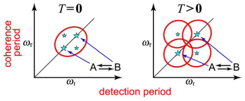
Schematic representation of 2D IR spectra of an overlapping pair of states in the presence of exchange.

The linear and 2D IR spectral line shapes may not be significantly modified by the exchange processes if the dephasing rate from population decay and frequency fluctuations of a given transition involved in exchange is fast compared with the exchange rate, which in turn may be slow in comparison with the peak frequency separation. This is analogous to the slow exchange limit of NMR although “slow” for the vibrational examples most often will mean picoseconds. In linear IR spectra there is only one time interval involved, a detection time, and the IR spectrum displays the Fourier transform of the free decay on this time axis. A single peak caused by fast transfer between two structures is not easily distinguishable from a peak arising from a continuous distribution of structures in linear IR. In 2D IR spectroscopy, however, the line widths along the anti-diagonal and the diagonal are different and change with population time and with temperature thereby exposing the exchange processes.

The exchange between species that have identifiably different mean frequencies under certain conditions is exemplified by a three-state system, representing the vibrational levels v = 0, 1, and 2 of a molecule imbedded in different environments A, B, etc. Each environment may give rise to a different potential surface and distributions of vibrational frequencies. This example may be quite common in ambient temperature solutions when previously undiscovered equilibrium dynamics are on the picosecond time scale.

The exchange that appears in the linear IR spectrum^169–172 is described by the half Fourier transform of $Re\left[n_{\text{A}}{\rho }_{01}^{(\text{A})}{\mu }_{10}^{(\text{A})}+n_B{\rho }_{01}^{(B)}{\mu }_{10}^{(B)}\right]$ where n_A and n_B are the equilibrium fractions of A and B. The vibrational coherences for species A and B having instantaneous vibrational frequencies ${\omega }_{01}^{(\text{A})}$ and ${\omega }_{01}^{(\text{B})}$ that are coupled by the forward and backward exchange rate coefficients k_AB and k_BA = k_ABe^ΔG_AB/k_BT are readily found analytically in terms of as averages of fixed frequencies ω̄, relaxation rate γ̄, exchange rate k̄ and the differences $\mathrm{\Delta }\overline{\omega }=({\omega }_{01}^{(\text{A})}-{\omega }_{01}^{(\text{B})})/2$, Δγ̄, and Δk̄ as:⁶⁶

$$\rho (\tau )=\langle \frac{1}{h}{e}^{a\tau }\left(\begin{array}{cc}hcosh(h\tau )+dsinh(h\tau )& (b-ic)sinh(h\tau )\\ (b+ic)sinh(h\tau )& hcosh(h\tau )-dsinh(h\tau )\end{array}\right)\rangle \rho (0)$$ (1.4)

where a = −iω̄ − γ̄ − k̄, b = k̄, c = −iΔk̄, d = −iΔω̄ − Δγ̄ − Δk̄, and $h=\sqrt{b^2+c^2+d^2}$. The angle brackets symbolize the integration over the distributions of frequencies. The very simple example c = 0 and d = iΔω̄ corresponds to the vibrational spectrum of two structures in dynamic equilibrium with a unit equilibrium constant. If the vibrators have equal populations and transition dipoles and the same pure dephasing rate, the following spectrum is predicted:

$$S(\omega )=Re\left\{{\left[i(\omega -\overline{\omega })+\overline{\gamma }+\frac{\mathrm{\Delta }{\overline{\omega }}^2}{i(\omega -\overline{\omega })+2\overline{k}+\overline{\gamma }}\right]}^{-1}\right\}$$ (1.5)

As a result of motional narrowing this spectrum displays two peaks when k̄ < Δω̄ and otherwise there is only one. In IR two identical peaks are not expected to merge symmetrically as the exchange rate increases. Although the forward and backward exchange rates of the two interchanging vibrators may be the same when there is no vibrational excitation they cannot then be equal in the v = 1 state; there is a difference in the free-energies associated with excited states of different species. The results show that linear spectroscopy will not identify the exchange when k̄ < Δω̄ unless the spectrum can be seen to vary with k̄, such as by varying the temperature. The situation is different for 2D IR which really exposes exchange in this limit.

A description of the 2D IR spectrum analogous to the foregoing treatment of linear IR involves the evolution of correlated coherences. In a mixture, each of the separate transitions in 2D IR has relative strength proportional to the mole fraction of a species. Since the linear absorption depends on the transition dipole squared, the 2D IR diagonal peaks depend on the fourth power while the cross peaks depend on the products of the squared dipoles of the involved structures, the comparison of these signals can be used to determine the ratio μ_A/μ_B.¹⁴⁹

The Liouville paths that contribute to the photon echo and nonrephasing signals when there is exchange are of the type: {(01)_A|(11)_A ⇄ (11)_B|(10)_A/B}and {(01)_A|(00)_A⇄ (00)_B|(10)_A/B} where (ab)_C represents a coherence ab in species C. A coherence (01)_A is introduced into the A-species by the first pulse in the sequence. The second pulse generates a population (11)_A or (00)_A which may undergo dynamic exchanges with (11)_B or (00)_B. Finally, the signal field is generated by a third pulse that forms the detected coherence in either of the species. These terms are modified by the kinetic factor P_AA as described below if A is the detected population and by P_AB when B is detected after some exchanges have occurred. Also included are the two quantum terms such as {(01)_A|(11)_A ⇄ (11)_B|(1+1,1)_A/B} involving v = 2 states, again with factors P_AA or P_AB depending on the kinetic outcome in the population period. An analogous set of diagrams consider the evolution to begin in state B. The spectral diffusion appears naturally in our simulation from those molecules that survive an exchange step during the measurement, such as the echo {(01)|(11)|(10)}_A where the same A- molecules undergoing spectral diffusion senses all four photon interactions. It is assumed that the spectral diffusion does not alter the magnitude of the integrated 2D IR diagonal signals which are considered to change only because of exchange and population relaxation processes and not because of changes in transition dipole with frequency (Condon approximation).

The diagonal signal S_AA for the A form at a given point in the two dimensional frequency space has a T-dependent shape with the content:

$$S_{\text{AA}}={\mu }_{\text{A}}^4{R}_{\text{AA}}({\omega }_{\tau },{\omega }_t;T)P_{\text{AA}}(T)N_{\text{A}}^{eq}$$ (1.6)

where R_AA(ω_τ, ω_t;T) is a 2D IR spectral shape factor arising from all the diagonal Liouville pathways contributing signal at that point including spectral diffusion. The cross peak signal S_AB in the same notation is:

$$S_{\text{AB}}={\mu }_{\text{A}}^2{\mu }_{\text{B}}^2{R}_{\text{AB}}({\omega }_{\tau },{\omega }_t;T)P_{\text{AB}}(T)N_{\text{A}}^{eq}$$ (1.7)

Each of these signals is associated with the relevant transition dipoles and the conditional probabilities P_AA (T), P_AB (T), P_BA (T) or P_BB (T) arising from kinetic equations. For the case that the T₁ times of the two species are equal these factors are:

$$P_{\text{AA}}(T)=\frac{k_{\text{AB}}}{2\overline{k}}{e}^{-T/T_1}(K_{eq}+e^{-2\overline{k}T})$$ (1.8)

$$P_{\text{AB}}(T)=\frac{k_{\text{AB}}}{2\overline{k}}{e}^{-T/T_1}(1-e^{-2\overline{k}T})$$ (1.9)

with the other two probabilities obtained by interchanging A and B. The ratio of the diagonal and cross peak signal areas is independent of T₁ and is a simple function of the exchange rate.

In the examples we have reported, the inverse of the vibrational line width has often been less than 500 fs, so an exchange time of a few picoseconds had a minor effect of the line shapes during the coherence and the detection periods. However, in the example of acetonitrile-methanol (see below) the rate of hydrogen-bond exchange was sufficiently increased at elevated temperatures:⁶⁶ to average the two IR transitions in the linear IR and cause the 2D IR transition shapes to be significantly altered. The kinetic factors are really evaluated numerically for any number of components having arbitrary population dynamics at equilibrium.

The dephasing dynamics, including spectral diffusion, can be introduced in a straightforward manner if the population kinetics is the same for all frequency groups associated with a particular configuration, for in that case (suppressing the transition dipole and hence the orientational dependence shown in eq 1.2) the v = 0 → v = 1 signals can be written in the form:

$$P_{\text{AB}}(T)e^{-\tau /2T_{1\text{A}}-t/2T_{1\text{B}}}\langle exp\left(\pm i{\int }_0^{\tau }{\omega }_{01}^{(\text{A})}(t^{\prime })d{t}^{\prime }-i{\int }_{\tau +T}^{\tau +T+t}{\omega }_{01}^{(\text{B})}(t^{\prime })d{t}^{\prime }\right)\rangle$$ (1.10)

where the example is given for rephasing (upper sign) and nonrephasing (lower sign) v = 0 → v = 1 pathways for molecules that have changed configuration during the population time T. As in previous examples the other responses only differ from eq 1.10 in their signs, and the choice of mean frequencies and their time evolution: they involve the overtones, combinations and fundamentals with their dynamics. For example, the case A = B the diagonal peaks of the regular 2D IR spectra of each species. The average in eq 1.10 is readily evaluated for Gaussian distributions of frequency deviations to yield the result:

$$P_{\text{AB}}(T)e^{-\tau /2T_{1\text{A}}-t/2T_{1\text{B}}}{e}^{\pm i{\omega }_{01}^{(\text{A})}\tau -i{\omega }_{01}^{(\text{B})}t+G_{\pm }(\tau ,T,t)}$$ (1.11)

where:

$$G_{\pm }(\tau ,T,t)=-g_{\text{AA}}(\tau )\pm g_{\text{AB}}(T)-g_{\text{BB}}(t)\mp g_{\text{AB}}(\tau +T)\mp g_{\text{AB}}(T+t)\pm g_{\text{AB}}(\tau +T+t)$$ (1.12)

and:

$$g_{\text{AB}}(t)={\int }_0^t{dt}_1{\int }_0^{t_1}{dt}_2\langle \delta {\omega }_{01}^{(\text{A})}(t_1)\delta {\omega }_{01}^{(\text{B})}(t_2)\rangle$$ (1.13)

The time evolution of the 2D IR spectral shapes is determined by the vibrational frequency time correlation functions in 1.11. For a classical oscillator all the Liouville paths¹²⁵ contribute to the spectrum as the Fourier transforms of terms of the type given in eq 1.11 where ω^(A) and ω^(B) are the time-dependent vibrational transition frequencies involved in the coherence and detection periods and the prefactor contains the population relaxation factors for these coherences. There have been many models proposed for the time correlations of these frequencies and numerous numerical computations of this relaxation function. A common assumption that achieves a simple model form for the phase accumulations assumes Gaussian distributions. In that case the spectrum depends only on two-time correlation functions of the frequencies which are often modeled by linear combinations of Kubo functions corresponding to overdamped Brownian oscillators,¹²⁵ sometimes combined with underdamped, oscillatory terms. These modeling procedures are approximate, but they serve to define the experimental signals in terms of parameters representative of the different time scales of the spectral relaxation and the variances of the underlying inhomogeneous distributions. The most quantitative approaches involve simulations of the full 2D IR signals based on molecular dynamics including quantum effects when necessary^7,8,160,173 to compute the accumulated phases in responses exemplified by eq 1.11.

The eq 1.12 shows clearly that when A and B have completely uncorrelated distributions there are no longer any line shape changes during the T interval so that the signal would have been obtained directly from:

$$P_{\text{AB}}(T)e^{-\tau /2T_{1\text{A}}-t/2T_{1\text{B}}}\langle exp\left(i{\int }_0^{\tau }{\omega }_{01}^{(\text{A})}(t^{\prime })d{t}^{\prime }\right)\rangle \langle exp\left(-i{\int }_{\tau +T}^{\tau +T+t}{\omega }_{01}^{(\text{B})}(t^{\prime })d{t}^{\prime }\right)\rangle$$ (1.14)

When the system is jumping back and forth between two states A and B, each delta pulse excitation initiates coherence in either A or B. So the conventional spectral diffusion G factor is involved only when the mean A-time (1/k_AB) or the mean B-time (1/k_BA) of the A/B trajectory is long enough that uninterrupted phase accumulation occurs in a single mode. In the foregoing summary the molecular rotation has been omitted. The overall rotation of the components in equilibrium during the coherence and detection periods also influences the line widths in 2D IR in a standard manner.^132,174 During the population period the specific form of the orientation factor for the various species in dynamic equilibrium depends on the kinetics of the their interchange, the Liouville paths and the orientational tensor component, <ZZZZ>, <XXZZ> or <ZXZX> that is chosen.^132,174

In principle the 2D IR signals depend on the kinetics undergone by the different populations storing the frequency information to be rephased. For example, the diagonal 2D IR contributions result from probing the ground (v = 0) and excited state (v = 1) populations through v = 0 → v = 1 transitions. However, the anharmonically shifted peak from the pathway {(01)_A|(11)_A|(21)_A} involves probing the v = 1 population through the v = 1 → v = 2 transition. The kinetic observables associated with these pathways are sensitive to any differences that may occur in the mechanisms of bleach recovery and excited-state population dynamics.⁷²

3. APPLICATIONS OF 2D IR TO HYDROGEN-BOND EXCHANGE PROCESSES

The 2D IR has proved useful in detecting equilibrium kinetics in a variety of examples mentioned earlier. In the following examples from this laboratory the examples of nitriles and carbonyls exchanging with hydrogen bonding solvents are described. Then two examples of discrete configurations of water interacting with peptides are discussed ending with a recent example of the conformational dynamics of a small tryptophan dipeptide.

Nitrile vibrations

¹⁷⁵ The vibrational spectra of nitriles have been used to probe local structures,^176–180 electric fields,^181–184, and solvent dynamics.^66,158,185 The localized –C ≡ N transitions are sufficiently sharp that small changes in frequency are readily quantified. Furthermore, nitriles can be introduced into proteins^182,183,186 and peptides^178,179,187 where their transitions are well removed from the peptide backbone infrared absorption. The physical origins of the nitrile peak shifts and line shapes have been examined theoretically.^188–190 For protein studies, the ability to connect the spectral shapes and frequencies of vibrational probes to specific structural and dynamical features remains an important challenge.

The 2D IR experiments^158,175,185 have clarified the nitrile vibrational dynamics. In each case the linear IR in methanol shows at least two transitions of the nitrile which are attributed to distributions of frequencies, one being more significantly hydrogen-bonded than the others. The nitrile solutes are approximated as forming two distributions of vibrational frequencies, one where they are mainly free (F) and the other, at higher frequency, where they are mainly hydrogen bonded (H) to methanol molecules. There is an equilibrium, H ⇄ F, between these two types of nitriles, with equilibrium constant K_eq = k_FH/k_HF.

Figure 7 illustrates the exchange results for acetonitrile in methanol and shows a typical kinetic trace obtained by measuring the relative areas of the diagonal and cross peaks in the 2D IR spectrum.¹⁵⁸ The exchange rates depend slightly on temperature. The H ⇄ F equilibrium constant yielded a ground state free-energy difference ΔG⁽⁰⁾ = 700 J·mol⁻¹ for acetonitrile and exchange rate coefficients k_HF = 0.086 ps⁻¹ at −17°C and 0.12 ps⁻¹ at 22°C suggesting a barrier of 5 kJ·mol⁻¹. These fast equilibrium kinetics are typical of those that can be measured by 2D IR. In the case of CH₃CN in methanol the exchanging frequency distributions were found to be uncorrelated. The dephasing rates and the exchange rates in that example are of the same order. Needless to say, the NMR transitions of two such exchanging states at equilibrium would be completely averaged into one transition.

Figure 7.

The real part of the absorptive 2D IR spectra of CH₃CN in MeOH and time evolution of the cross peaks in 2D IR. (a) 2D IR spectra with waiting times of T =0 and T =15 ps at −17°C.¹⁵⁸ (b) Three-dimensional views of v =0 →v =1 region of 2D IR spectra of CH₃CN in MeOH with waiting times of T = 0, T = 2ps, T = 6 ps, and T = 15 ps at −17 °C (middle) and pictorial representations of ongoing hydrogen-bond exchange during waiting time (left and right). (c) Relative magnitudes at 22°C (*) and −17°C (+) of the cross-to-diagonal peak ratio versus T in the v =0 →v =1 region.¹⁵⁸

In recent work¹⁷⁵ we have characterized the equilibrium hydrogen-bond dynamics for the aromatic nitriles benzonitrile (BN) and cinnamonitrile (CIN) which are the building blocks of the reverse transcriptase inhibitors whose 2D IR was recently reported¹⁸⁵ and that will be mentioned again later. The time constants of hydrogen-bond exchange, shown in Figure 8, for these aromatic nitriles (2k̄ = 0.19 ps⁻¹ and 0.22 ps⁻¹ for BN and CIN, respectively) are faster than for acetonitrile. The 2D IR spectra were simulated (Figure 8e and f) for CIN using a frequency correlation function:

$$\langle \omega (t)·\omega (0)\rangle =\gamma \delta (t)+{\sigma }^2+{\mathrm{\Delta }}^2{e}^{-t/\tau }$$ (1.15)

which includes a motionally narrowed contribution (γ), a fixed inhomogeneous part (σ) and spectral diffusion expressed by two parameters Δ and τ for both F and H. The data were consistent with the exchange destroying the frequency correlation as discussed above. The parameters that give an adequate fit for the linear spectrum and reproduce the principal experimental features of the 2D IR spectra are: γ_F = 0.18; γ_H = 0.19; σ_F =0.37; σ_H = 0.41; Δ_F = 0.14; Δ_H = 0.35; (all in ps⁻¹) and τ_F = 2.1; τ_H = 2.6; (in ps). The simulated spectra illustrate clearly that the 2D IR is dominated by the effects of exchange which creates the asymmetric shape due to the evolution of strong underlying cross peaks. It is also apparent from the simulation that the transitions are undergoing spectral diffusion in addition to exchange. The spectral diffusion causes the peaks to be significantly more rounded after a waiting time. The spectral diffusion times τ_H and τ_F are conjectured to arise from field fluctuations at the CN of CIN caused by varying configurations of H-bonds between methanol molecules that are not H bonding to the solute. The general features are the same for benzonitrile are the same as those found for CIN. The results for both BN and CIN suggest that the transition dipole is increased upon formation of the hydrogen bond and that in both cases the F state is more stable than the H state. Similar results have also been seen for dipeptides whose phenylalanine is replaced by p-cyanophenyl alanine.¹⁷⁵

Figure 8.

Benzonitrile and cinnamonitrile 2D IR spectra at T =0 and T =6 ps in MeOH. 2D IR spectra of benzonitrile at (a) T =0 and (b) and T =6 ps. 2D IR spectra of cinnamonitrile at (c) T =0 and (d) T =6 ps. Simulated 2D IR spectra of cinnamonitrile at (e) T =0 and (f) T =6 ps.¹⁷⁵

This information regarding the time scales of the picosecond equilibrium dynamics of the nitriles with methanol is not available from linear spectroscopy. The 2D IR clearly exposes the presence of picosecond equilibrium exchanges of dominantly two states. The evolution of the cross peaks in 2D IR due to exchange is easily distinguishable from anharmonic coupling of a single vibrator, which would give a cross peak even at T = 0, a well-known property of coupled anharmonic oscillators.¹⁹¹ In the present examples there are no cross peaks formed at T = 0 except those attributable to the finite width of the excitation pulses, so anharmonic coupling is not the explanation of the vibrational peaks in methanol.

The waiting-time dependence of 2D IR spectra readily distinguishes these additional bands from Fermi resonances. When there is a pronounced Fermi resonance, the linear spectrum displays two transitions but the 2D IR spectra of Fermi resonant pairs¹⁹² will display strong cross peaks at T = 0. The cross peaks at T = 0 are very small for all of the aforementioned nitriles in methanol. The additional structure in the nitrile stretching mode when the solvent is methanol is not reproduced by the CN stretching mode in water suggesting that the vibrational transitions of the various H-bonded structures of CN and liquid water are dynamically averaged, meaning that for water structure exchange k̄ ≫ Δω̄ in eq 1.5.

2D IR of a nonnucleoside inhibitor complexed with HIV-1 reverse transcriptase

¹⁸⁵ The nitrile fundamental vibration has a transition dipole of ca. 0.1 D compared with ca. 0.50 D for the amide-I modes. Since the 2D IR responses vary as the dipole to the fourth power the nitrile may give signals that are up to hundreds of time weaker than amide-I. This factor is diminished somewhat by the narrower IR line width of nitrile compared with amide-I in some environments. Nevertheless the excellent sensitivity of 2D IR makes it possible to observe nitriles at few mM concentrations, suitable for studies of labeled peptides and proteins.¹⁸⁵ As examples we discuss the results for an enzyme inhibitor complex that incorporates the model benzo- and cinnamo- nitriles whose 2D IR spectra are shown in Figure 8 to be undergoing chemical exchange of hydrogen bonds.¹⁷⁵ They are both molecular components of some HIV-1 reverse transcriptase (RT) inhibitors that have been discovered and structurally characterized by Arnold and coworkers.¹⁹³ The function of RT is to enable the conversion of a single-stranded RNA into a double-stranded DNA in a step that is essential for viral replication. The nonnucleoside inhibitors of HIV-1 RT (NNRTIs) bind in a hydrophobic pocket between two β-sheets.¹⁹⁴ It has been suggested that the binding of certain NNRTI inhibitors may be resistant to mutation-induced changes in the protein sequence.¹⁹⁵ Therefore, the 2D IR of the CN vibrations responding to motions of the drug and the nearby residues has great biological interest. The 2D IR echo method is expected to sense the fluctuating fields created by motions proximate and distant protein atoms as well as protein associated water.

Although the cyanovinyl CN group stretching transition is at lower frequency and has a three times higher integrated absorption cross-section than that of benzonitrile in most solvents, the TMC278 inhibitor (see Figure 9) always exhibits a single IR absorption peak indicating that the stretching mode of both nitriles peaks at the same frequency, However the 2D IR spectra of the inhibitor complex indicate (see Figure 10) the presence of two transitions in the nitrile stretch region, with the stronger one at lower frequency. These two bands have therefore been attributed to the two arms of the drug. The 2D IR results reveal significant heterogeneity in the nitrile frequencies which undergo fast spectral diffusion. The elongation of the 2D IR spectrum along the diagonal evident from Figure 10 implies that there is a distribution of CN frequencies corresponding to a distribution of polarities. The T dependence of the changes in the shape of the spectrum reports on the relaxation of this distribution. At small T values, the shapes of the 2D IR v = 0 → 1 bands resemble ellipses elongated close to the diagonal line, but as T increases to 3 ps the peaks become more circular. The frequency correlations can be followed by a quantitative analysis of these spectral shape changes from which it has been shown¹⁸⁵ that the correlation function decays on two time scales: a fast process of 130 fs that is not so well determined and a slow one in the range of 7 ps (see Figure 10e). The simulation of the vibrational mode dynamics in Figure 10e is based on a correlation function consisting of a pair of Kubo functions with one of them in a motional narrowing limit, that is

Figure 9.

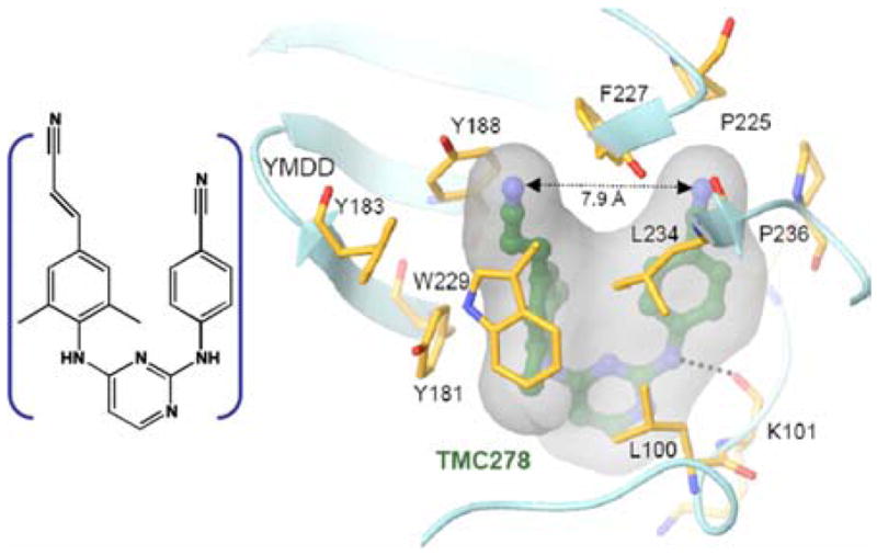
Structure at 1.8-Å resolution of the HIV-1 reverse transcriptase enzyme RT52A complexed with the NNRTI drug TMC278 (19). (Left) The inhibitor. (Right) A simplified view of TMC278 in the binding pocket. The dashed line connects the cyanovinyl and benzonitrile CN groups. The cyanovinyl arm extends into a hydrophobic tunnel formed by the side chains of Tyr-181, Tyr-188, Phe-227, Leu-234, and Trp-229.¹⁸⁵

Figure 10.

(a)–(d): 2D correlation spectra of the HIV-1 RT/TMC278 complex in aqueous buffer solution with the following waiting times: T =200 fs (a), T =500 fs (b), T =1 ps (c), and T =3 ps (d). The nitrile stretching modes of the two drug wings are indicated by dashed lines at ω_τ = 2214.5 cm⁻¹ and 2227.2 cm⁻¹, respectively. (e) The ultrafast dynamics of the v =0 →1 transition of the cyanovinyl nitrile stretching mode of the HIV-1 RT/TMC278 complex. An elliptical parameter describing the 2D IR shape M(T) vs. T plot (circles) is least-squares fitted by a biexponential with time constants 130 fs and 7ps.¹⁸⁵

$$\langle {\omega }_{01}(t)·{\omega }_{01}(0)\rangle =-\gamma t-{\mathrm{\Delta }}^2{e}^{-t/{\tau }_c}$$ (1.16)

The cyanovinyl arm of the drug occupies a hydrophobic tunnel formed by the side chains of Tyr-181, Tyr-188, Phe-227, Leu-234, and Trp-229 as illustrated in Figure 9. The overall decay of the correlation should require relaxation of this local environment of the CN groups.

The 2D IR proved to have excellent sensitivity in this example. Both CN groups were readily distinguished in the spectra at protein concentrations around a few mM. Both transitions exhibited a distribution of frequencies and had similar T₁ relaxation times of ca. 3 ps. The two arms of the drug are demonstrably in different protein environments and the cyanovinyl arm relaxes its nitrile stretching frequency distribution (τ_c) on the tens-of-picosecond time scale, thereby providing a means to visualize the structural fluctuations of the protein interior.

Water exchange with amide and carbonyl modes

The effects of chemical exchange have also been observed in the 2D IR spectral shapes for aqueous amide-I or carbonyls having apparently single vibrational bands in FTIR. Their population evolution exposes discrete distributions undergoing ps time scale exchange. The FTIR spectra of Trpzip2 (Gly-7 ¹³C=¹⁶O) shows a spectral separation between residue 7 and the remaining peptide making it possible to probe the dynamics of the solvent directly in contact with a particular residue (see Figure 11). Major structural alterations of this peptide are expected to be much slower than a few picoseconds. The total shift of the carbonyl frequency due to H-bonding is ca. 30–40 cm⁻¹.¹⁶⁰ The Gly-7 peaks bracket a range of 35 cm⁻¹, which is well within expectations for different H-bonded configurations ranging from those that are on average free from H-bonding at the highest frequencies to those with on average three optimally bonded water molecules at the lowest frequencies. The water hydrogen-bond dynamics around the Gly-7 residue is manifested by the fast interchange between these configurations.

Figure 11.

Linear and 2D IR spectra of tryptophan zipper-2 β-hairpin (Trpzip2, Ser1-Trp2-Thr3-Trp4-Glu5-Asn6-Gly7-Lys8-Trp9-Thr10-Trp11-Lys12) isotopically labeled with ¹³C=¹⁶O at Gly7 in D₂O and its molecular structure. (Left) The linear IR spectrum and the 2D IR spectra at T =0 and T =1ps are shown from the top. (Right) Molecular structure of Trpzip2, the linear IR spectrum, and 2D IR spectra at T =0, T =500 fs, and T =1 ps in the isotope region are shown from the top. The 2D IR spectra at T =0 and T =1 ps on the right side are enlarged views of the region enclosed by dotted squares in their corresponding 2D IR spectra on the left side. All the 2D IR spectra represent real absorptive spectra and were collected at room temperature with <ZZZZ> tensor components.¹⁰⁹

The substates composing the Gly-7 residue amide-I′ band of Trpzip2 have peak frequencies of 1607, 1595, 1583, and 1572 cm⁻¹. In all of the cases investigated a qualitative comparison of the cross peak trace with the diagonal 2D IR spectra shows that the latter manifest undulations in the regions of these same substates. The 2D IR spectra at large population time were numerically fit to the components from the different substates seen in the trace and the cross peaks that develop between them. Such fitting for Trpzip2 indicates that the fast dynamics observed in the diagonal peak region of the Gly-7 amide-I′ mode at T =1 ps is caused by the ca. 0.5 to 1.5 ps time scale interchange between the three substates with the highest peak frequencies. The CO···H radial distributions obtained from MD simulations¹⁹⁶ show a strong residue dependence. The dependence of local water structure on peptide residue will be discussed below with reference to the alanine dipeptide.

It has been mentioned that similar expressions as described above for exchange would be used if there were energy transfer between two states of each molecule whether they derive from Fermi resonances or they correspond to different fundamental modes. It is well known that in polypeptides there will be energy transfer between the spatially separated amide-I modes, if there are fluctuations in their coupling.^106,197,198 However, the 2D IR spectra differ in important detail whether the cross peaks derive from exchange, energy transfer or Fermi resonances.

An example that qualitatively illustrates a number of these features of the dynamics is the diketone piperidone which displays mode-selective vibrational energy transfer from the ester carbonyl to the cis-amide and also exchange dynamics on individual transitions.¹⁰⁹ As the population time increases from T =0 to T =2 ps the diagonal peaks of both carbonyl groups change their shape from being diagonally elongated to a more square shape shown in Figure 12. The unusual square shape is attributed to the presence of cross peaks from exchange between substates, or population distributions, having different diagonal frequencies, similar to the cartoon of Figure 6 which is for two such states. The ester carbonyl group presents the most varied example. The substates of the C=O stretch of the ester in water arise from two sources, both of which have mechanisms to fluctuate the vibrational frequency: the single bond rotamers separated by few kcal/mol barriers that permit ps exchanges; and various configurations of water molecules which are H-bonded to the ester carbonyl group. Figure 12 shows the dependence of the 2D spectra of piperidone in D₂O on the waiting time and tensor components. The relative magnitudes of both types of cross peaks, one from energy transfer appearing in the upper left and lower right of each 2D spectrum and the other from H-bond exchange appearing in the diagonal peak region, increases as the waiting time increases. For the cross peaks originating from energy transfer, the magnitude and sign show strong dependence on polarizations. With <XXZZ> the cross peaks are most pronounced. In addition, for the <ZXXZ> polarization, the signs of the cross peaks are inverted and much weaker than in other conditions. The diagonal peak shape changes at later waiting times, however, are independent of the tensor components. Therefore, the dependence of the 2D IR spectra on the waiting time and tensor choice help confirm the origins of the cross peaks.

Figure 12.

2D IR spectra of piperidone (see inset in (a)) in D₂O at different waiting times and polarizations. Real part of the 2D absorptive spectra with <ZZZZ> polarization, at (a) T =0, (b) T =1 ps, (c) T =2 ps, and (d) T =4 ps. (e) <XXZZ> polarization at T =0 and (f) <XXZZ> with T =2 ps. (g) <ZXXZ> polarization at T =0 and (h) T =2 ps. In each spectrum the white area corresponds to a flat top off-scale signal. In all the spectra the contours begin at 60% of the peak signals. The areas highlighted by a small square in (h) are 10-times intensified.¹⁴⁷

The tryptophan dipeptide

The tryptophan dipeptide (NATMA) in D₂O shows two conformers having distinctive acetyl-end amide-I′ transition frequencies.¹⁹⁹ This spectral structure is more clearly resolved in 2D IR than in FTIR. In two-dimensional echo spectroscopy cross peaks between these conformer transitions show they are undergoing exchange on the 1.5 ps time scale. The molecular dynamics simulations show that the dipeptide is undergoing angular motions around the C_α–C_β and the C_β–C_γ single bonds that alter the proximity of the acetyl-end amide group and the indole ring. Figure 13 shows the two extreme structures.¹⁹⁹ The single-bond rotation around C_α–C_β makes the hydrophobic indole ring become more proximate to the carbonyl carbon of the acetyl end in one of the conformational distributions centered at 4.0 Å. The water (D₂O) structure around the acetyl amide unit is then modified as compared with the other conformer.

Figure 13.

Structures and 2D IR spectra of tryptophan dipeptide in D₂O. (a) Newman projection of two extremes of the C_α–C_β single bond rotation obtained from MD simulations. (b) 2D IR spectra of acetyl (C_ac) amide-I mode at T = 0. (c) 2D IR at T =1ps.¹⁹⁹

The multiple transitions of the acetyl-end amide-I′ mode in the 2D IR spectra of tryptophan dipeptide in D₂O indicate the existence of two conformational distributions, each having a spectrally distinct vibrational peak, one at 1630 cm⁻¹ (A) and the other at 1643 cm⁻¹ (B) that undergo a 1.0 ps chemical exchange. A simplified kinetic model, consistent with a computation of the IR spectrum and molecular dynamics simulations explains the results:

$$\underset{\mathit{decay}}{\overset{T_{1\text{A}}}{\leftarrow }}\text{A}(1630{\text{cm}}^{-1})\underset{k_{\text{BA}}}{\overset{k_{\text{AB}}}{\rightleftarrows }}\text{B}(1643{\text{cm}}^{-1})\underset{\mathit{decay}}{\overset{T_{1\text{B}}}{\to }}$$ (1.17)

The diagonal 2D IR signal S_AA for the state A at a given point in the two dimensional frequency space has the content ${\mu }_{\text{A}}^4{R}_{\text{AA}}({\omega }_{\tau },{\omega }_t;T)P_{\text{AA}}(T)N_{\text{A}}^{eq}$ where R_AA(ω_τ, ω_t; T) is a 2D IR spectral shape factor arising from all the Liouville pathways^200,201 contributing at that point and $N_{\text{A}}^{eq}$ the equilibrium number density of A. The cross peak signal S_AB in the same notation is ${\mu }_{\text{A}}^2{\mu }_{\text{B}}^2{R}_{\text{AB}}({\omega }_{\tau },{\omega }_t;T)P_{\text{AB}}(T)N_{\text{A}}^{eq}$. The ratio of the diagonal and cross peak signal areas can be approximated by a simple function of the exchange rate:

$$S_{\text{AB}}/S_{\text{AA}}=\frac{{\mu }_{\text{B}}^2(1-e^{-2\overline{k}T})}{{\mu }_{\text{A}}^2(K_{eq}+e^{-2\overline{k}T})}$$ (1.18)

The cross peak centered at (ω_τ =1630 cm⁻¹, ω_t =1643 cm⁻¹; K_eq =2 (295K)) and the diagonal peak at 1630 cm⁻¹. A detailed study of the waiting-time dependence and fitting based on the assumption there is exchange between only two states having equal transition dipoles evidences a value of 1/2k̄ of 1.5 ps.¹⁹⁹

The sensitivity of the amide-I′ modes to hydrogen bonding is well known.^202,203 The usual qualitative picture of H-bonding of the amide group is that on average there are three water molecules bound- one to the N-H and two to the C=O.²⁰⁴ The frequency distributions of the amide-I modes of the alanine dipeptide, calculated from the MD trajectories using SPECTRON,²⁰⁵ show a broad asymmetric distribution for the acetyl end and a narrower symmetric distribution for the N-methylamino end. The proximity of the indole ring to the acetyl-end C=O and N-H influences the hydrogen bonding of the water molecules. The spectrum of the acetyl end with two or more hydrogen bonds (as defined by a simple algorithm¹⁹⁹) were significantly down shifted (−10 cm⁻¹) from that with fewer than two hydrogen bonds, showing that the calculated asymmetry is arising from a distribution of H-bond structures. The ultrafast rotations around the single bonds cause alternating changes in the solvent (H-bonding) environment of the acetyl-end amide group, giving rise to the two frequency distributions in the 2D spectra.

The hydrogen-bond dynamics between the acetyl-end C=O and the surrounding water molecules were also obtained from MD by computing 〈h(0)h(t)〉/〈h²〉,^206,207 where h(t) =1 if one particular water molecule within the first shell is hydrogen bonded and zero if it is not (again using a simple distance and angle algorithm). The simulated correlation function, which is the sum of the contributions from all the water molecules, has an ultrafast component that decays in 100 fs., the time scale predicted²⁰⁸ for the librational motions. It also decays on a timescale of 6.2 × 10¹¹ s⁻¹, which describes the structural relaxation of the hydrogen bonds of the dipeptide. This rate is close to the measured exchange rate.

The results of this recent work have provided¹⁹⁹ direct experimental evidence that the water structure and its dynamics in the neighborhood of an exposed amide unit depends significantly on the hydrophobic character of the nearby residue. It is likely that this factor will require to be considered in descriptions of the dynamics of water near proteins, as already shown in some simulations.²⁰⁹

MD simulations indicate that on the few-picosecond time scale there is significant back-and-forth motion of the indole ring caused by axial rotations about the C-C single bonds. Simulated structural features have bimodal distributions suggesting that there are two dominant peaks in the equilibrium structure distribution consistent with the presence of at least two peaks in the frequency distribution. The variations of the water structure around the carbonyl also track these molecular motions suggesting that it is the changes in the H-bond configurations that cause the vibrational frequency shifts. In one group of conformations the indole ring appears to offer more hydrophobic protection of the acetyl-end carbonyl, which would result in the blue shift of its vibrational frequency.

4. THE VIBRATIONAL EXCITATIONS IN AMYLOID FIBRILS²⁰⁷

In the foregoing examples the ions, peptides or buried probes are undergoing relatively fast dynamics. We now discuss the application of 2D IR to fibrils in which the amide units would be thought to be relatively free from picosecond motions. However, it will be seen that they are undergoing slow structural changes as well as fast spectral diffusion that is dependent on which residue is examined. Amyloid fibrils accumulate as plaques in the brain tissue of persons with Alzheimer’s disease. They are composed primarily of β-amyloid (Aβ) peptides that range in length from 39 to 42 residues. Our 2D IR experiments concern the fibrils from the 40-residue peptide Aβ40 for which structural models have been developed by Tycko and co-workers.^210,211 They feature parallel in-register β-sheets involving residues 9–24 and 30–40 and a loop region usually involving 23–29. A monofilament is formed by folding of each peptide chain and two such monofilaments comprise the fibril (Figure 14a). The ordered structure of these fibrils extends to macroscopic length scales, so the vibrational states of the fibrils differ from those of small molecules or globular proteins.

Figure 14.

Diagrams of Aβ40 fibrils. (a) A cross section of two laterally displaced molecular layers of the Aβ40 fibril according to Petkova et al.²¹⁰ Residues 9–40 are shown. (b) Idealized structure of a portion of the parallel β-sheet. The strands are indicated by s, and the residue number in a given strand is indicated by n. The ¹³C=¹⁸O-labeled carbonyl groups are shown in red.²¹³

The vibrational excitations of an extended system as exhibited by these fibrils can be significantly altered by isotope substitution of the repeat units. The isotope shift between ¹²C=¹⁶O and ¹³C=¹⁸O carbonyl vibrational transitions is large compared with the exciton interactions between them at van der Waals distances and longer. Thus, a two- or three-dimensional vibrational exciton can be induced to form arrays having reduced dimensionality.²¹² Therefore, experiments at various isotopic contents will expose the underlying properties of the vibrational excitation topology of a macroscopic array. The amyloid fibril presents a beautiful example of this phenomenon. A β-sheet structure forms two-dimensional excitons. However, if one of the residues of each peptide chain has a single ¹³C=¹⁸O substitution, the replaced groups will form a linear array along the fibril axis (Figure 15b). The vibrational exciton topology for the isotope region is thereby reduced to a nearly one-dimensional chain. The spectra of linear chains are quantum mechanically tractable and a quantitative analysis of the spectra–structure relationships should be obtainable from them. When the natural and ¹³C=¹⁸O substituted Aβ40 polypeptides are mixed in known proportions the spectra become those of disordered linear chains. Our recent paper reported 2D IR spectra of a range of such mixtures,²¹³ which have confirmed that indeed nearly linear chains are formed.

Figure 15.

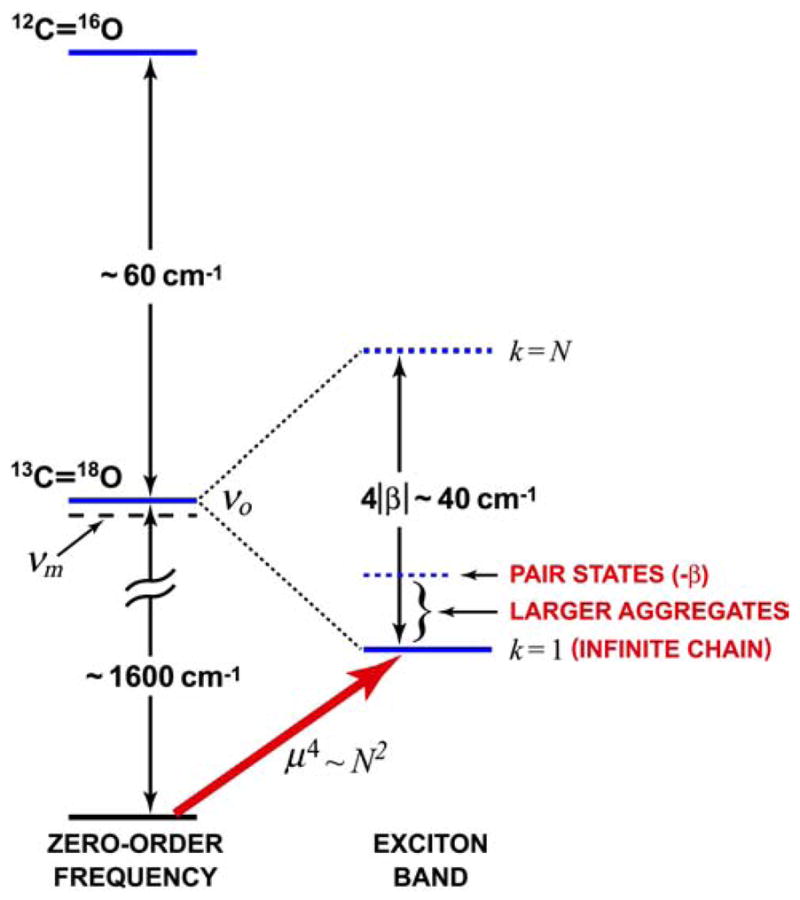
Schematic representation of the energy levels for isotopically dilute linear excitons.

Linear-chain vibrational excitations have predictable spectra

The spectra of perfect linear-chain vibrational excitons have qualitatively similar characteristics for nearest neighbor coupling and longer range interactions, so they are adequately illustrated for the former case where the frequencies are well known to be:

$$E_K/h{c}_o={\nu }_K={\nu }_o+2\beta cosK$$ (1.19)

with K = πk/(N +1) and k = 1 to N for N interacting monomers having a coupling β (cm⁻¹). The transition dipole moment squared from the vibrational ground state to the K^th state of the perfect lattice, ${\mu }_K^2$, is dominated by the state with k = 1. When N ≫ 1 this domination amounts to >80%.^212,214,215 In that case the frequency-integrated absorption coefficient of the chain of N residues is ca. 0.8N times that of a single amide unit. The photon echo signal varies as the fourth power of the transition dipole moment,¹²⁵ so its peak signal scales approximately as N². The k =1 state is the lowest-energy state of the linear chain exciton when the nearest neighbor coupling constant dominates and is negative when the dipoles are arranged approximately in a head-to-tail manner. Therefore, the approximate linear chains created by isotope substitution at a strand residue are each expected to exhibit an intense, vibrational transition in 2D IR that is shifted to lower frequency by 2β from ν_o as illustrated in Figure 15.

The transition corresponding to the frequency ν_o is present at infinite isotope dilution if the spectrum consists of isolated ¹³C=¹⁸O molecules that do not resonantly couple to any neighboring amide groups but are nevertheless shifted from the gas frequency by the intermolecular potential including electrostatic interactions. The most dilute system we have examined is 5% ¹³C=¹⁸O molecules in ¹²C=¹⁶O fibrils which consists of mainly of monomers at approximately ν_m = ν_o − 2β²/|Δ_iso|, where Δ_iso (cm⁻¹) is the isotope shift of 60 cm⁻¹. The situation is significantly altered when higher percentages of isotope substitution are used. The relevant system then becomes a linear chain that is disordered by intermittent energy-mismatched sites. The 2D IR spectra in the region of the v =1 transitions are estimated from the same principles as just given for the linear IR spectra, by simulating rephasing diagrams {(0K) (K′ K) (K′0)} and {(0K) (00) (K′0)} and their nonrephasing counterparts for all K with inclusion of the local vibrational dephasing and population dynamics by using information from smaller peptides. The main prediction of the effect of isotopic dilution of a linear-chain exciton by 50% is a broadening and a shift to higher frequency caused by a disorder-induced redistribution of the k = 1 amplitude and this is exactly what was depicted by the experiments.²¹³ The experimental shifts provided estimates of the interstack distances. Assuming the exciton band is formed from a point dipole–dipole potential,⁴ the repeat separations between the dipoles were found to be 0.51 ± 0.04 nm (Ala-21), 0.48 ± 0.04 nm (Gly-29), 0.49 ± 0.03 nm (Gly-33), and 0.53 ± 0.06 nm (Gly-38). These values compare remarkably well with NMR measurements that indicated a 0.48 ± 0.05-nm repeat distance between the backbone carbonyl carbons in the parallel in-register regions of the fibrils.²¹⁶ In these examples the 2D IR is used to measure frequencies with high sensitivity but it should be realized that these same experiments are readily applicable to follow kinetics of the amyloid structures.

The improved sensitivity of 2D IR compared with linear IR is demonstrated in Figure 16 by comparing spectra of G38* of a matured Aβ40 sample (note that the asterisk identifies the residue that has ¹³C=¹⁸O substitution). The trace of the 2D IR spectrum along a line close to the diagonal shows separated peaks that are unresolved in the linear IR spectrum. The spectral resolution of 2D IR improves at finite waiting times because the contribution of inhomogeneous broadening to the line width decreases as shown in one of the examples given below.

Figure 16.

Linear and 2D IR spectra of fibrils of Aβ40 labeled with ¹³C=¹⁸O at Gly-38 after 19 days of maturation. (a) Linear IR spectrum (blue) and a trace along the dotted line ω_t= ω_τ +2 cm⁻¹ of the 2D IR spectrum shown in (b) (red). The dotted circle in (a) highlights the isotope-labeled amide-I transition region. (b) An absorptive 2D IR spectrum at T =200 fs.

2D IR exposes a residue-dependent heterogeneity of the fibrils

The 2D IR signals expose novel properties the fibrils. The 2D IR spectra of G38*, G33*, G29*, A21*, as reported earlier²¹³ and also V39*, G37*, L34*, I32*, I31*, V24*, F20*, F19*, L17*, V18*, and V12* from more recent work²¹⁷ are all similar but have interesting differences. For example, G29* displays two sharp bands separated by 12 cm⁻¹ in the isotope region as shown in Figure 17. There is a cross peak between these two bands in the 2D IR evidenced by the nearly vertical appearance of the v =1 →v =2 transition region (Figure 17b). This result strongly suggests that the two peaks represent vibrational transitions in a single fibril. The large variations in spectral shifts of the amide-I′ modes for different residues clearly reveals microscopic heterogeneity of the couplings responsible for the exciton bands. The analysis by isotope-dilution methods has shown that the vibrational excitation exchange couplings and dimensionality of the exciton bands are similar at each of the sites that were examined.²¹³ However, large frequency shifts of the exciton transitions of as much as 18 cm⁻¹ occur. These appear to be residue-dependent changes in ν_o (defined in Figure 15). A possible reason for these shifts is the heterogeneous character of the electric field along the chain carbonyl groups. In a related example, the frequencies of isotopically substituted transitions in a β-hairpin were shown to be very sensitive to the electric field at the particular amide group¹⁹⁶ arising from other residues of the backbone and from the surrounding water molecules. The experimental shifts for A21*, G29*, G33*, and G38* were qualitatively consistent with estimates of the electric field along the carbonyl group calculated from a continuum model for the electrostatic interactions.²¹⁸ The partial charges on the residues neighboring the linear chains, for example, the charged lysine neighboring Gly-29, make important contributions to this field which varies by as much as 24 MV/cm at different residues.

Figure 17.

2D IR spectra of fibrils of ¹³C=¹⁸O-labeled Gly-25 (G25*) (a) and ¹³C=¹⁸O-labeled Gly-29 (G29*) (b) at T =0 after 70 days of maturation. In each spectrum the white area corresponds to a flat top off-scale signal. The contours begin at 25% of the peak signals. The Insets are enlarged and 10-times-intensified in (a) and two-times-intensified in (b) views of the marked areas.²¹³

In recent work we have investigated the shifts of the lowest-energy-allowed exciton transitions for a much wider range of ¹³C=¹⁸O substituted fibrils.²¹⁷ The results are summarized in Figure 18. Each isotopomer shows a main transition with weaker side bands. As before, transitions are significantly more distinctive in 2D IR than in FTIR. The variation of vibrational frequency with residue is not obviously correlated with residue location. Since it is very likely that these shifts represent variations in ν_o it will be most interesting to have a full theoretical analysis of the vibrational spectra of fibrils that incorporates the actual local structure, the variations in the electrostatic field and the field gradients at each of the ¹³C=¹⁸O coupled amide-I modes.

Figure 18.

Variation in the peak frequency of ¹³C=¹⁸O-labeled residues of Aβ40 fibrils.

Fast dynamics in fibrils

Much of the foregoing discussion assumes the fibril structure is rigid but the electric field at the amide units is not expected to be static. For some residues there is a significant time dependence of the vibrational frequency. One such example is Leucine17* shown in Figure 19. At T = 2 ps the spectral diffusion has removed some inhomogeneous broadening to reveal clearly that there are underlying peaks in the distribution. This fast spectral diffusion could be from restricted motions of charged side chains or possibly from motions of water molecules that have been incorporated during the fibrillization process.²¹³

Figure 19.

Spectral diffusion of vibrational spectra of mature fibrils of Aβ40: 2D IR spectra of the ¹³C=¹⁸O-labeled Leu-17 (L17*) amide-I mode at (a) T =0 and (b) T =2 ps.

The maturation of fibrils can be tracked by 2D IR

Besides the ultrafast spectral diffusion processes discussed above there are also slower kinetics being undergone by these fibrils that can be seen by 2D IR. The kinetics and mechanism of the aggregation process of Aβ proteins to prefibrillar structures is a very important issue for the study of Alzheimer’s disease. The 2D IR method is proving to be a useful tool to investigate such folding processes.²¹⁹

In addition to the variations of the transition frequency residue by residue that are summarized in Figure 18, there are interesting changes seen at different maturation times in our spectra (Figure 20). The signals are sensitive to the presence of intermediate structures involved in fibrillization. The slow time evolution of well-aligned linear chains along the fibril axis of Aβ40 varies residue by residue. Based on results from Aβ40 fibrils, it is conjectured that Gly-38 residues tend to form linear-chain exciton transitions earlier than do the Gly-33 or Gly-29 residues. During the aggregation process the evolution of the β-sheet structure is readily exemplified from the 2D IR spectra of L34* in Figure 20.²¹⁷ The random coil and β-sheet structures are the peaks in the range of 1640 to1650 cm⁻¹ and 1620 to 1630 cm⁻¹, respectively. The <XXZZ> tensor spectra in Figure 20c shows the well-developed β-sheet structures most clearly from the cross peaks highlighted by solid squares. In the early stages of the aggregation the 2D IR signal magnitude of Leu-34 increases by a factor of 3 indicating a sudden structural change in the vicinity this residue. These features²¹⁷ again dramatize the sensitivity of 2D IR to the structural evolution of such aggregates.

Figure 20.

2D IR spectra of L34* in solution during aggregation and matured fibrils in solid fibrils. (a–c) The 2D IR spectra of L34* with the aggregation tome of 0 hour (before the aggregation) (a), 1 hour (b), and 30 hours (c). All the 2D IR data were obtained with the sample temperature at 22°C except the 0 hour data which was collected with the sample temperature of 4°C and in all the spectra the contours begin at 80% of the peak signals.²¹⁷

5. CONCLUSIONS AND PROSPECTS

A few recent examples from this laboratory of two-dimensional infrared echo spectroscopy accompanied by a brief survey of by now well-known principles of nonlinear spectroscopy have been presented in this Feature Article. In the few years since the first 2D IR pump/probe and 2D IR echo spectroscopic experiments,^5,18 there have been an amazing variety of highly significant, previously unforeseen advances and applications based on these principles. Other methods of 2D IR are also proving to have wide application, such as the quasi steady-state approaches of Wright and coworkers²²⁰ that are now being applied in proteomics.²²¹ While infrared spectroscopy has long been understood by experts to manifest the signatures of complex molecular structures, too much of the essential information is hidden in conventional spectra. The multi-dimensional spectroscopic results are exposing hitherto unseen features and will lead us to new levels of quantitative analysis of vibrational spectra and its relation to structural dynamics in condensed phases. The combination of structure and fast dynamics exposed by these methods is enabling major advances in the visualization of the behavior of complex systems.

References

- 1.Kapteyn H, Cohen O, Christov I, Murnane M. Science. 2007;317:775. doi: 10.1126/science.1143679. [DOI] [PubMed] [Google Scholar]
- 2.Krimm S, Bandekar J. Adv Protein Chem. 1986;38:181. doi: 10.1016/s0065-3233(08)60528-8. [DOI] [PubMed] [Google Scholar]
- 3.Dong A, Huang P, Caughey WS. Biochemistry. 1990;29:3303. doi: 10.1021/bi00465a022. [DOI] [PubMed] [Google Scholar]
- 4.Torii H, Tasumi M. J Chem Phys. 1992;96:3379. [Google Scholar]
- 5.Hamm P, Lim M, Hochstrasser RM. J Phys Chem B. 1998;102:6123. [Google Scholar]
- 6.Cha SY, Ham SH, Cho MH. J Chem Phys. 2002;117:740. [Google Scholar]
- 7.Schmidt JR, Corcelli SA, Skinner JL. J Chem Phys. 2004;121:8887. doi: 10.1063/1.1791632. [DOI] [PubMed] [Google Scholar]
- 8.Hayashi T, Zhuang W, Mukamel S. J Phys Chem A. 2005;109:9747. doi: 10.1021/jp052324l. [DOI] [PubMed] [Google Scholar]
- 9.Piryatinski A, Tretiak S, Chernyak V, Mukamel S. J Raman Spectrosc. 2000;31:125. [Google Scholar]
- 10.Scheurer C, Piryatinski A, Mukamel S. J Am Chem Soc. 2001;123:3114. doi: 10.1021/ja003412g. [DOI] [PubMed] [Google Scholar]
- 11.Choi JH, Ham S, Cho M. J Chem Phys. 2002;117:6821. [Google Scholar]
- 12.Ham S, Hahn S, Lee C, Kim TK, Kwak K, Cho M. J Phys Chem B. 2004;108:9333. [Google Scholar]
- 13.Dijkstra AG, Knoester J. J Phys Chem B. 2005;109:9787. doi: 10.1021/jp044141p. [DOI] [PubMed] [Google Scholar]
- 14.Torii H. J Phys Chem A. 2006;110:4822. doi: 10.1021/jp060014c. [DOI] [PubMed] [Google Scholar]
- 15.Schweitzer-Stenner R. Biophys J. 2002;83:523. doi: 10.1016/S0006-3495(02)75188-6. [DOI] [PMC free article] [PubMed] [Google Scholar]
- 16.Demirdoven N, Cheatum CM, Chung HS, Khalil M, Knoester J, Tokmakoff A. J Am Chem Soc. 2004;126:7981. doi: 10.1021/ja049811j. [DOI] [PubMed] [Google Scholar]
- 17.Fang C, Senes A, Cristian L, DeGrado WF, Hochstrasser RM. Proc Natl Acad Sci U S A. 2006;103:16740. doi: 10.1073/pnas.0608243103. [DOI] [PMC free article] [PubMed] [Google Scholar]
- 18.Asplund MC, Zanni MT, Hochstrasser RM. Proc Natl Acad Sci U S A. 2000;97:8219. doi: 10.1073/pnas.140227997. [DOI] [PMC free article] [PubMed] [Google Scholar]
- 19.Shim SH, Strasfeld DB, Ling YL, Zanni MT. Proc Natl Acad Sci U S A. 2007;104:14197. doi: 10.1073/pnas.0700804104. [DOI] [PMC free article] [PubMed] [Google Scholar]
- 20.Nee MJ, McCanne R, Kubarych KJ, Joffre M. Opt Lett. 2007;32:713. doi: 10.1364/ol.32.000713. [DOI] [PubMed] [Google Scholar]
- 21.DeFlores LP, Nicodemus RA, Tokmakoff A. Opt Lett. 2007;32:2966. doi: 10.1364/ol.32.002966. [DOI] [PubMed] [Google Scholar]
- 22.DeMaria AJ, Stetser DA, Heynau H. Appl Phys Lett. 1966;8:1746. [Google Scholar]
- 23.Shank CV, Ippen EP. Appl Phys Lett. 1974;24:373. [Google Scholar]
- 24.Gruebele M, Wolynes PG. Acc Chem Res. 2004;37:261. doi: 10.1021/ar030230t. [DOI] [PubMed] [Google Scholar]
- 25.Laubereau A, Kaiser W. Rev Mod Phys. 1978;50:607. [Google Scholar]
- 26.Oxtoby DW. Adv Chem Phys. 1979;40:1. [Google Scholar]
- 27.Greene BI, Hochstrasser RM, Weisman RB. J Chem Phys. 1979;70:1247. [Google Scholar]
- 28.Ippen EP, Shank CV, Lewis A, Marcus MA. Science. 1978;200:1279. doi: 10.1126/science.663607. [DOI] [PubMed] [Google Scholar]
- 29.Greene BI, Hochstrasser RM, Weisman RB, Eaton WA. Proc Natl Acad Sci U S A. 1978;75:5255. doi: 10.1073/pnas.75.11.5255. [DOI] [PMC free article] [PubMed] [Google Scholar]
- 30.Legay F. Vibrational relaxation in matrices. Vol. 2 Academic Press; New York: 1977. [Google Scholar]
- 31.Rice SA. Adv Chem Phys. 1981;47:117. [Google Scholar]
- 32.Zwanzig R. J Chem Phys. 1961;34:1931. [Google Scholar]
- 33.Decola PL, Hochstrasser RM, Trommsdorff HP. Chem Phys Lett. 1980;72:1. [Google Scholar]
- 34.Hesp BH, Wiersma DA. Chem Phys Lett. 1980;75:423. [Google Scholar]
- 35.Trout TJ, Velsko S, Bozio R, Decola PL, Hochstrasser RM. J Chem Phys. 1984;81:4746. [Google Scholar]
- 36.Owrutsky JC, Raftery D, Hochstrasser RM. Annu Rev Phys Chem. 1994;45:519. doi: 10.1146/annurev.pc.45.100194.002511. [DOI] [PubMed] [Google Scholar]
- 37.Fork RL, Greene BI, Shank CV. Appl Phys Lett. 1981;38:671. [Google Scholar]
- 38.Dantus M, Rosker MJ, Zewail AH. J Chem Phys. 1987;87:2395. [Google Scholar]
- 39.Fourkas JT, Fayer MD. Acc Chem Res. 1992;25:227. [Google Scholar]
- 40.Moore JN, Hansen PA, Hochstrasser RM. Chem Phys Lett. 1987;138:110. [Google Scholar]
- 41.Anfinrud PA, Han C, Hochstrasser RM. Proc Natl Acad Sci U S A. 1989;86:8387. doi: 10.1073/pnas.86.21.8387. [DOI] [PMC free article] [PubMed] [Google Scholar]
- 42.Owrutsky JC, Kim YR, Li M, Sarisky MJ, Hochstrasser RM. Chem Phys Lett. 1991;184:368. [Google Scholar]
- 43.Maiti S, Walker GC, Cowen BR, Pippenger R, Moser CC, Dutton PL, Hochstrasser RM. Proc Natl Acad Sci U S A. 1994;91:10360. doi: 10.1073/pnas.91.22.10360. [DOI] [PMC free article] [PubMed] [Google Scholar]
- 44.Heilweil EJ, Casassa MP, Cavanagh RR, Stephenson JC. Chem Phys Lett. 1985;117:185. doi: 10.1103/PhysRevLett.64.2090. [DOI] [PubMed] [Google Scholar]
- 45.Heilweil EJ, Casassa MP, Cavanagh RR, Stephenson JC. J Chem Phys. 1986;85:5004. [Google Scholar]
- 46.Heilweil EJ, Casassa MP, Cavanagh RR, Stephenson JC. Annu Rev Phys Chem. 1989;40:143. [Google Scholar]
- 47.Bader JS, Berne BJ. J Chem Phys. 1994;100:8359. [Google Scholar]
- 48.Whitnell RM, Wilson KR, Hynes JT. J Phys Chem. 1990;94:8625. [Google Scholar]
- 49.Benjamin I, Whitnell RM. Chem Phys Lett. 1993;204:45. [Google Scholar]
- 50.Gnanakaran S, Hochstrasser RM. J Chem Phys. 1996;105:3486. [Google Scholar]
- 51.Yarne DA, Tuckerman ME, Klein ML. Chem Phys. 2000;258:163. [Google Scholar]
- 52.Kuo CH, Vorobyev DY, Chen J, Hochstrasser RM. J Phys Chem B. 2007;111:14028. doi: 10.1021/jp076503+. [DOI] [PubMed] [Google Scholar]
- 53.Anfinrud PA, Han CH, Lian TQ, Hochstrasser RM. J Phys Chem. 1991;95:574. [Google Scholar]
- 54.Dougherty TP, Grubbs WT, Heilweil EJ. J Phys Chem. 1994;98:9396. [Google Scholar]
- 55.Hamm P, Zinth W. J Phys Chem. 1995;99:13537. [Google Scholar]
- 56.Owrutsky JC, Baronavski AP. J Chem Phys. 1996;105:9864. [Google Scholar]
- 57.Asbury JB, Ellingson RJ, Ghosh HN, Ferrere S, Nozik AJ, Lian T. J Phys Chem B. 1999;103:3110. [Google Scholar]
- 58.Kobayashi T, Salto T, Ohtani H. Nature. 2001;414:531. doi: 10.1038/35107042. [DOI] [PubMed] [Google Scholar]
- 59.Herbst J, Heyne K, Diller R. Science. 2002;297:822. doi: 10.1126/science.1072144. [DOI] [PubMed] [Google Scholar]
- 60.van Thor Jasper J, Zanetti G, Ronayne Kate L, Towrie M. J Phys Chem B. 2005;109:16099. doi: 10.1021/jp051315+. [DOI] [PubMed] [Google Scholar]
- 61.Stoner-Ma D, Melief EH, Nappa J, Ronayne KL, Tonge PJ, Meech SR. J Phys Chem B. 2006;110:22009. doi: 10.1021/jp065326u. [DOI] [PubMed] [Google Scholar]
- 62.Kolano C, Helbing J, Kozinski M, Sander W, Hamm P. Nature. 2006;444:469. doi: 10.1038/nature05352. [DOI] [PubMed] [Google Scholar]
- 63.Asbury JB, Hao EC, Wang YQ, Lian TQ. J Phys Chem B. 2000;104:11957. [Google Scholar]
- 64.Owrutsky JC, Culver JP, Li M, Kim YR, Sarisky MJ, Yeganeh MS, Yodh AG, Hochstrasser RM. J Chem Phys. 1992;97:4421. [Google Scholar]
- 65.Khalil M, Demirdoven N, Tokmakoff A. J Chem Phys. 2004;121:362. doi: 10.1063/1.1756870. [DOI] [PubMed] [Google Scholar]
- 66.Kim YS, Hochstrasser RM. J Phys Chem B. 2006;110:8531. doi: 10.1021/jp060935n. [DOI] [PMC free article] [PubMed] [Google Scholar]
- 67.Rickard MA, Pakoulev AV, Kornau K, Mathew NA, Wright JC. J Phys Chem A. 2006;110:11384. doi: 10.1021/jp063917e. [DOI] [PubMed] [Google Scholar]
- 68.Graener H, Seifert G, Laubereau A. Phys Rev Lett. 1991;66:2092. doi: 10.1103/PhysRevLett.66.2092. [DOI] [PubMed] [Google Scholar]
- 69.Woutersen S, Emmerichs U, Bakker HJ. Science. 1997;278:658. [Google Scholar]
- 70.Laenen R, Rauscher C, Laubereau A. Phys Rev Lett. 1998;80:2622. [Google Scholar]
- 71.Bakker HJ, Nienhuys HK. Science. 2002;297:587. doi: 10.1126/science.1073298. [DOI] [PubMed] [Google Scholar]
- 72.Stenger J, Madsen D, Hamm P, Nibbering ETJ, Elsaesser T. J Phys Chem A. 2002;106:2341. [Google Scholar]
- 73.Fecko CJ, Eaves JD, Loparo JJ, Tokmakoff A, Geissler PL. Science. 2003;301:1698. doi: 10.1126/science.1087251. [DOI] [PubMed] [Google Scholar]
- 74.Asbury JB, Steinel T, Stromberg C, Corcelli SA, Lawrence CP, Skinner JL, Fayer MD. J Phys Chem A. 2004;108:1107. doi: 10.1063/1.1803532. [DOI] [PMC free article] [PubMed] [Google Scholar]
- 75.Cowan ML, Bruner BD, Huse N, Dwyer JR, Chugh B, Nibbering ETJ, Elsaesser T, Miller RJD. Nature. 2005;434:199. doi: 10.1038/nature03383. [DOI] [PubMed] [Google Scholar]
- 76.Lim M, Gnanakaran S, Hochstrasser RM. J Chem Phys. 1997;106:3485. [Google Scholar]
- 77.Hamm P, Lim M, Hochstrasser RM. J Chem Phys. 1997;107:10523. [Google Scholar]
- 78.Hamm P, Lim M, Hochstrasser RM. Phys Rev Lett. 1998;81:5326. [Google Scholar]
- 79.Lim M, Hamm P, Hochstrasser RM. Proc Natl Acad Sci U S A. 1998;95:15315. doi: 10.1073/pnas.95.26.15315. [DOI] [PMC free article] [PubMed] [Google Scholar]
- 80.Cavanagh RR, Germer TA, Stephenson JC. Vib Spectrosc. 1995;9:77. [Google Scholar]
- 81.Smits M, Ghosh A, Sterrer M, Muller M, Bonn M. Phys Rev Lett. 2007:98. doi: 10.1103/PhysRevLett.98.098302. [DOI] [PubMed] [Google Scholar]
- 82.Beckerle JD, Cavanagh RR, Casassa MP, Heilweil EJ, Stephenson JC. J Chem Phys. 1991;95:5403. doi: 10.1103/PhysRevLett.64.2090. [DOI] [PubMed] [Google Scholar]
- 83.Ghosh HN, Asbury JB, Lian TQ. J Phys Chem B. 1998;102:6482. [Google Scholar]
- 84.Phillips CM, Mizutani Y, Hochstrasser RM. Proc Natl Acad Sci U S A. 1995;92:7292. doi: 10.1073/pnas.92.16.7292. [DOI] [PMC free article] [PubMed] [Google Scholar]
- 85.Lim M, Jackson TA, Anfinrud PA. Science. 1995;269:962. doi: 10.1126/science.7638619. [DOI] [PubMed] [Google Scholar]
- 86.Rector KD, Engholm JR, Rella CW, Hill JR, Dlott DD, Fayer MD. J Phys Chem A. 1999;103:2381. [Google Scholar]
- 87.Chung HS, Khalil M, Smith AW, Ganim Z, Tokmakoff A. Proc Natl Acad Sci U S A. 2005;102:612. doi: 10.1073/pnas.0408646102. [DOI] [PMC free article] [PubMed] [Google Scholar]
- 88.Mukherjee P, Kass I, Arkin I, Zanni MT. Proc Natl Acad Sci U S A. 2006;103:3528. doi: 10.1073/pnas.0508833103. [DOI] [PMC free article] [PubMed] [Google Scholar]
- 89.Kleiman VD, Arrivo SM, Melinger JS, Heilweil EJ. Chem Phys. 1998;233:207. [Google Scholar]
- 90.Ventalon C, Fraser JM, Vos MH, Alexandrou A, Martin JL, Joffre M. Proc Natl Acad Sci U S A. 2004;101:13216. doi: 10.1073/pnas.0401844101. [DOI] [PMC free article] [PubMed] [Google Scholar]
- 91.Strasfeld DB, Shim SH, Zanni MT. Phys Rev Lett. 2007:99. doi: 10.1103/PhysRevLett.99.038102. [DOI] [PubMed] [Google Scholar]
- 92.Fujisaki H, Straub JE. Proc Natl Acad Sci U S A. 2005;102:6726. doi: 10.1073/pnas.0409083102. [DOI] [PMC free article] [PubMed] [Google Scholar]
- 93.Yoo HS, McWhorter DA, Pate BH. J Phys Chem A. 2004;108:1380. [Google Scholar]
- 94.Heilweil EJ, Doany FE, Moore R, Hochstrasser RM. J Chem Phys. 1982;76:5632. [Google Scholar]
- 95.Rey R, Hynes JT. J Chem Phys. 1998;108:142. [Google Scholar]
- 96.Li M, Owrutsky J, Sarisky M, Culver JP, Yodh A, Hochstrasser RM. J Chem Phys. 1993;98:5499. [Google Scholar]
- 97.Polak M, Gruebele M, Saykally RJ. J Am Chem Soc. 1987;109:2884. [Google Scholar]
- 98.Li S, Schmidt JR, Skinner JL. J Chem Phys. 2006;125:244507/1. doi: 10.1063/1.2408421. [DOI] [PubMed] [Google Scholar]
- 99.Morita A, Kato S. J Chem Phys. 1998;109:5511. [Google Scholar]
- 100.Kim YS, Hochstrasser RM. J Phys Chem B. 2005;109:6884. doi: 10.1021/jp0449511. [DOI] [PubMed] [Google Scholar]
- 101.DeCamp MF, DeFlores L, McCracken JM, Tokmakoff A, Kwac K, Cho M. J Phys Chem B. 2005;109:11016. doi: 10.1021/jp050257p. [DOI] [PubMed] [Google Scholar]
- 102.Sul S, Karaiskaj D, Jiang Y, Ge NH. J Phys Chem B. 2006;110:19891. doi: 10.1021/jp062039h. [DOI] [PubMed] [Google Scholar]
- 103.Nguyen PH, Stock G. J Chem Phys. 2003;119:11350. [Google Scholar]
- 104.Rubtsov IV, Wang J, Hochstrasser RM. J Phys Chem A. 2003;107:3384. [Google Scholar]
- 105.Park J, Hochstrasser RM. Chem Phys. 2006;323:78. [Google Scholar]
- 106.Rubtsov IV, Hochstrasser RM. J Phys Chem B. 2002;106:9165. [Google Scholar]
- 107.DeFlores LP, Ganim Z, Ackley SF, Chung HS, Tokmakoff A. J Phys Chem B. 2006;110:18973. doi: 10.1021/jp0603334. [DOI] [PubMed] [Google Scholar]
- 108.Kurochkin DV, Naraharisetty SRG, Rubtsov IV. Proc Natl Acad Sci U S A. 2007;104:14209. doi: 10.1073/pnas.0700560104. [DOI] [PMC free article] [PubMed] [Google Scholar]
- 109.Kim YS, Hochstrasser RM. J Phys Chem B. 2007;111:9697. doi: 10.1021/jp074267x. [DOI] [PubMed] [Google Scholar]
- 110.Botan V, Backus EHG, Pfister R, Moretto A, Crisma M, Toniolo C, Nguyen PH, Stock G, Hamm P. Proc Natl Acad Sci U S A. 2007;104:12749. doi: 10.1073/pnas.0701762104. [DOI] [PMC free article] [PubMed] [Google Scholar]
- 111.Gordon JP, Wang CH, Patel CKN, Slusher RE, Tomlinson WJ. Phys Rev. 1969;179:294. [Google Scholar]
- 112.Aartsma TJ, Wiersma DA. Phys Rev Lett. 1976;36:1360. [Google Scholar]
- 113.Bigot JY, Portella MT, Schoenlein RW, Bardeen CJ, Migus A, Shank CV. Phys Rev Lett. 1991;66:1138. doi: 10.1103/PhysRevLett.66.1138. [DOI] [PubMed] [Google Scholar]
- 114.Berg M, Walsh CA, Narasimhan LR, Littau KA, Fayer MD. J Chem Phys. 1988;88:1564. [Google Scholar]
- 115.Broer MM, Golding B, Haemmerle WH, Simpson JR, Huber DL. Phys Rev B. 1986;33:4160. doi: 10.1103/physrevb.33.4160. [DOI] [PubMed] [Google Scholar]
- 116.Webb MD, Cundiff ST, Steel DG. Phys Rev Lett. 1991;66:934. doi: 10.1103/PhysRevLett.66.934. [DOI] [PubMed] [Google Scholar]
- 117.Narasimhan LR, Bai YS, Dugan MA, Fayer MD. Chem Phys Lett. 1991;176:335. [Google Scholar]
- 118.Meijers HC, Wiersma DA. Phys Rev Lett. 1992;68:381. doi: 10.1103/PhysRevLett.68.381. [DOI] [PubMed] [Google Scholar]
- 119.Zimdars D, Tokmakoff A, Chen S, Greenfield SR, Fayer MD, Smith TI, Schwettman HA. Phys Rev Lett. 1993;70:2718. doi: 10.1103/PhysRevLett.70.2718. [DOI] [PubMed] [Google Scholar]
- 120.Hamm P, Lim M, DeGrado WF, Hochstrasser RM. J Phys Chem A. 1999;103:10049. [Google Scholar]
- 121.Joo T, Jia Y, Yu JY, Lang MJ, Fleming GR. J Chem Phys. 1996;104:6089. [Google Scholar]
- 122.Zanni MT, Asplund MC, Hochstrasser RM. J Chem Phys. 2001;114:4579. [Google Scholar]
- 123.Cervetto V, Helbing J, Bredenbeck J, Hamm P. J Chem Phys. 2004;121:5935. doi: 10.1063/1.1778163. [DOI] [PubMed] [Google Scholar]
- 124.Tanimura Y, Mukamel S. J Chem Phys. 1993;99:9496. [Google Scholar]
- 125.Mukamel S. Principles of Nonlinear Optical Spectrscopy. Oxford Univ. Press; New York: 1995. [Google Scholar]
- 126.Mukamel S. Annu Rev Phys Chem. 2000;51:691. doi: 10.1146/annurev.physchem.51.1.691. [DOI] [PubMed] [Google Scholar]
- 127.Hamm P, Hochstrasser RM. Structure and dynamics of proteins and peptides: femtosecond two-dimensional infrared spectroscopy. In: Fayer MD, editor. Ultrafast Infrared and Raman Spectroscopy. Vol. 26. Marcel Dekker, Inc; New York: 2001. p. 273. [Google Scholar]
- 128.Sung J, Silbey RJ. J Chem Phys. 2001;115:9266. [Google Scholar]
- 129.Khalil M, Demirdoven N, Tokmakoff A. Phys Rev Lett. 2003;90:047401/1. doi: 10.1103/PhysRevLett.90.047401. [DOI] [PubMed] [Google Scholar]
- 130.Jonas DM. Annu Rev Phys Chem. 2003;54:425. doi: 10.1146/annurev.physchem.54.011002.103907. [DOI] [PubMed] [Google Scholar]
- 131.Cho M. Chem Rev. 2008;108:1331. doi: 10.1021/cr078377b. [DOI] [PubMed] [Google Scholar]
- 132.Hochstrasser RM. Chem Phys. 2001;266:273. [Google Scholar]
- 133.Ge NH, Zanni MT, Hochstrasser RM. J Phys Chem A. 2002;106:962. [Google Scholar]
- 134.Hochstrasser RM. Adv Chem Phys. 2006;132:1. [Google Scholar]
- 135.Zheng J, Kwak K, Fayer MD. Acc Chem Res. 2007;40:75. doi: 10.1021/ar068010d. [DOI] [PubMed] [Google Scholar]
- 136.Tian P, Keusters D, Suzaki Y, Warren WS. Science. 2003;300:1553. doi: 10.1126/science.1083433. [DOI] [PubMed] [Google Scholar]
- 137.Shim SH, Strasfeld DB, Fulmer EC, Zanni MT. Opt Lett. 2006;31:838. doi: 10.1364/ol.31.000838. [DOI] [PubMed] [Google Scholar]
- 138.Rubtsov IV, Wang J, Hochstrasser RM. Proc Natl Acad Sci U S A. 2003;100:5601. doi: 10.1073/pnas.0931292100. [DOI] [PMC free article] [PubMed] [Google Scholar]
- 139.Nibbering ETJ, Elsaesser T. Chem Rev. 2004;104:1887. doi: 10.1021/cr020694p. [DOI] [PubMed] [Google Scholar]
- 140.Fulmer EC, Mukherjee P, Krummel AT, Zanni MT. J Chem Phys. 2004;120:8067. doi: 10.1063/1.1649725. [DOI] [PubMed] [Google Scholar]
- 141.Cho M. Bull Korean Chem Soc. 2006;27:1940. [Google Scholar]
- 142.Golonzka O, Tokmakoff A. J Chem Phys. 2001;115:297. [Google Scholar]
- 143.Woutersen S, Hamm P. J Phys Chem B. 2000;104:11316. [Google Scholar]
- 144.Woutersen S, Hamm P. J Chem Phys. 2001;114:2727. [Google Scholar]
- 145.Kim YS, Wang J, Hochstrasser RM. J Phys Chem B. 2005;109:7511. doi: 10.1021/jp044989d. [DOI] [PubMed] [Google Scholar]
- 146.Bagchi S, Kim YS, Charnley AK, Smith AB, III, Hochstrasser RM. J Phys Chem B. 2007;111:3010. doi: 10.1021/jp067348m. [DOI] [PubMed] [Google Scholar]
- 147.Kim YS, Hochstrasser RM. Pacific Grove/CA, USA. July 30 - August 4, 2006; Ultrafast Phenomena XV, Springer series in chemical physics; 2007. p. 332. [Google Scholar]
- 148.Hamm P, Woutersen S. Bull Chem Soc Jpn. 2002;75:985. [Google Scholar]
- 149.Fang C, Wang J, Kim YS, Charnley AK, Barber-Armstrong W, Smith AB, III, Decatur SM, Hochstrasser RM. J Phys Chem B. 2004;108:10415. [Google Scholar]
- 150.Fang C, Hochstrasser RM. J Phys Chem B. 2005;109:18652. doi: 10.1021/jp052525p. [DOI] [PubMed] [Google Scholar]
- 151.Maekawa H, Toniolo C, Moretto A, Broxterman QB, Ge NH. J Phys Chem B. 2006;110:5834. doi: 10.1021/jp057472q. [DOI] [PubMed] [Google Scholar]
- 152.Maekawa H, Toniolo C, Broxterman QB, Ge NH. J Phys Chem B. 2007;111:3222. doi: 10.1021/jp0674874. [DOI] [PubMed] [Google Scholar]
- 153.Maekawa H, Formaggio F, Toniolo C, Ge NH. J Am Chem Soc. 2008;130:6556. doi: 10.1021/ja8007165. [DOI] [PubMed] [Google Scholar]
- 154.Rubtsov IV, Wang J, Hochstrasser RM. J Chem Phys. 2003;118:7733. [Google Scholar]
- 155.Rubtsov IV, Kumar K, Hochstrasser RM. Chem Phys Lett. 2005;402:439. [Google Scholar]
- 156.Kumar K, Sinks LE, Wang J, Kim YS, Hochstrasser RM. Chem Phys Lett. 2006;432:122. [Google Scholar]
- 157.Lazonder K, Pshenichnikov MS, Wiersma DA. Opt Lett. 2006;31:3354. doi: 10.1364/ol.31.003354. [DOI] [PubMed] [Google Scholar]
- 158.Kim YS, Hochstrasser RM. Proc Natl Acad Sci U S A. 2005;102:11185. doi: 10.1073/pnas.0504865102. [DOI] [PMC free article] [PubMed] [Google Scholar]
- 159.Woutersen S, Mu Y, Stock G, Hamm P. Chem Phys. 2001;266:137. doi: 10.1073/pnas.201169498. [DOI] [PMC free article] [PubMed] [Google Scholar]
- 160.Kwac K, Lee H, Cho M. J Chem Phys. 2004;120:1477. doi: 10.1063/1.1633549. [DOI] [PubMed] [Google Scholar]
- 161.Zheng J, Kwak K, Chen X, Asbury JB, Fayer MD. J Am Chem Soc. 2006;128:2977. doi: 10.1021/ja0570584. [DOI] [PubMed] [Google Scholar]
- 162.Kwak K, Park S, Fayer MD. Proc Natl Acad Sci U S A. 2007;104:14221. doi: 10.1073/pnas.0701710104. [DOI] [PMC free article] [PubMed] [Google Scholar]
- 163.Zheng J, Kwak K, Xie J, Fayer MD. Science. 2006;313:1951. doi: 10.1126/science.1132178. [DOI] [PubMed] [Google Scholar]
- 164.Cahoon JF, Sawyer KR, Schlegel JP, Harris CB. Science. 2008;319:1820. doi: 10.1126/science.1154041. [DOI] [PubMed] [Google Scholar]
- 165.Schmidt JR, Corcelli SA, Skinner JL. J Chem Phys. 2005;123:044513/1. doi: 10.1063/1.1961472. [DOI] [PubMed] [Google Scholar]
- 166.Loparo JJ, Roberts ST, Tokmakoff A. J Chem Phys. 2006;125:194521/1. doi: 10.1063/1.2382895. [DOI] [PubMed] [Google Scholar]
- 167.Lindner J, Voehringer P, Pshenichnikov MS, Cringus D, Wiersma DA, Mostovoy M. Chem Phys Lett. 2006;421:329. [Google Scholar]
- 168.Ha JH, Kim YS, Hochstrasser RM. J Chem Phys. 2006;124:064508/1. doi: 10.1063/1.2162165. [DOI] [PubMed] [Google Scholar]
- 169.Kreevoy MM, Mead CA. J Am Chem Soc. 1962;84:4596. [Google Scholar]
- 170.Turner JJ, Grevels FW, Howdle SM, Jacke J, Haward MT, Klotzbuecher WE. J Am Chem Soc. 1991;113:8347. [Google Scholar]
- 171.Turner JJ, Gordon CM, Howdle SM. J Phys Chem. 1995;99:17532. [Google Scholar]
- 172.Londergan CH, Kubiak CP. Chem Eur J. 2003;9:5962. doi: 10.1002/chem.200305028. [DOI] [PubMed] [Google Scholar]
- 173.Noid WG, Loring RF. J Chem Phys. 2005;122:174507/1. doi: 10.1063/1.1888485. [DOI] [PubMed] [Google Scholar]
- 174.Golonzka O, Khalil M, Demirdoven N, Tokmakoff A. Phys Rev Lett. 2001;86:2154. doi: 10.1103/PhysRevLett.86.2154. [DOI] [PubMed] [Google Scholar]
- 175.Ghosh A, Remorino A, Tucker MJ, Hochstrasser RM. Chem Phys Lett. doi: 10.1016/j.cplett.2008.12.094. In press. [DOI] [PMC free article] [PubMed] [Google Scholar]
- 176.Eaton G, Pena-Nunez AS, Symons MCR. J Chem Soc Faraday Trans 1. 1988;84:2181. [Google Scholar]
- 177.Fawcett WR, Liu G, Kessler TE. J Phys Chem. 1993;97:9293. [Google Scholar]
- 178.Getahun Z, Huang CY, Wang T, De Leon B, DeGrado WF, Gai F. J Am Chem Soc. 2003;125:405. doi: 10.1021/ja0285262. [DOI] [PubMed] [Google Scholar]
- 179.Tucker MJ, Getahun Z, Nanda V, DeGrado WF, Gai F. J Am Chem Soc. 2004;126:5078. doi: 10.1021/ja032015d. [DOI] [PubMed] [Google Scholar]
- 180.Krummel AT, Zanni MT. J Phys Chem B. 2008;112:1336. doi: 10.1021/jp711558a. [DOI] [PubMed] [Google Scholar]
- 181.Andrews SS, Boxer SG. J Phys Chem A. 2000;104:11853. [Google Scholar]
- 182.Suydam IT, Boxer SG, Park ES, Romanova ZS. Biophys J. 2002;82:186. [Google Scholar]
- 183.Suydam IT, Boxer SG. Biophys J. 2005;88:159A. [Google Scholar]
- 184.Fafarman AT, Webb LJ, Chuang JI, Boxer SG. J Am Chem Soc. 2006;128:13356. doi: 10.1021/ja0650403. [DOI] [PMC free article] [PubMed] [Google Scholar]
- 185.Fang C, Baumann JD, Das K, Remorino A, Arnold E, Hochstrasser RM. Proc Natl Acad Sci U S A. 2008;105:1472. doi: 10.1073/pnas.0709320104. [DOI] [PMC free article] [PubMed] [Google Scholar]
- 186.Schultz KC, Supekova L, Ryu Y, Xie J, Perera R, Schultz PG. J Am Chem Soc. 2006;128:13984. doi: 10.1021/ja0636690. [DOI] [PubMed] [Google Scholar]
- 187.Mukherjee S, Chowdhury P, DeGrado WF, Gai F. Langmuir. 2007;23:11174. doi: 10.1021/la701686g. [DOI] [PubMed] [Google Scholar]
- 188.Choi JH, Oh KI, Lee H, Lee C, Cho M. J Chem Phys. 2008:128. doi: 10.1063/1.2844787. [DOI] [PubMed] [Google Scholar]
- 189.Oh KI, Choi JH, Lee JH, Han JB, Lee H, Cho M. J Chem Phys. 2008:128. doi: 10.1063/1.2904558. [DOI] [PubMed] [Google Scholar]
- 190.Lindquist BA, Corcelli SA. J Phys Chem B. 2008;112:6301. doi: 10.1021/jp802039e. [DOI] [PubMed] [Google Scholar]
- 191.Woutersen S, Pfister R, Hamm P, Mu Y, Kosov DS, Stock G. J Chem Phys. 2002;117:6833. [Google Scholar]
- 192.Edler J, Hamm P. J Chem Phys. 2003;119:2709. [Google Scholar]
- 193.Das K, Bauman JD, Clark AD, Frenkel YV, Lewi PJ, Shatkin AJ, Hughes SH, Arnold E. Proc Natl Acad Sci U S A. 2008;105:1466. doi: 10.1073/pnas.0711209105. [DOI] [PMC free article] [PubMed] [Google Scholar]
- 194.Jacobo-Molina A, Ding J, Nanni RG, Clark AD, Jr, Lu X, Tantillo C, Williams RL, Kamer G, Ferris AL, et al. Proc Natl Acad Sci U S A. 1993;90:6320. doi: 10.1073/pnas.90.13.6320. [DOI] [PMC free article] [PubMed] [Google Scholar]
- 195.Das K, Clark AD, Jr, Lewi PJ, Heeres J, De Jonge MR, Koymans LMH, Vinkers HM, Daeyaert F, Ludovici DW, Kukla MJ, De Corte B, Kavash RW, Ho CY, Ye H, Lichtenstein MA, Andries K, Pauwels R, De Bethune M-P, Boyer PL, Clark P, Hughes SH, Janssen PAJ, Arnold E. J Med Chem. 2004;47:2550. doi: 10.1021/jm030558s. [DOI] [PubMed] [Google Scholar]
- 196.Wang J, Zhuang W, Mukamel S, Hochstrasser R. J Phys Chem B. 2008;112:5930. doi: 10.1021/jp075683k. [DOI] [PMC free article] [PubMed] [Google Scholar]
- 197.Gnanakaran S, Hochstrasser RM. J Am Chem Soc. 2001;123:12886. doi: 10.1021/ja011088z. [DOI] [PubMed] [Google Scholar]
- 198.Woutersen S, Mu Y, Stock G, Hamm P. Proc Natl Acad Sci U S A. 2001;98:11254. doi: 10.1073/pnas.201169498. [DOI] [PMC free article] [PubMed] [Google Scholar]
- 199.Bagchi S, Charnley AK, Smith AB, III, Hochstrasser RM. In process. [Google Scholar]
- 200.Sanda F, Mukamel S. J Chem Phys. 2006;125:014507/1. doi: 10.1063/1.2205367. [DOI] [PubMed] [Google Scholar]
- 201.Kwak K, Zheng J, Cang H, Fayer MD. J Phys Chem B. 2006;110:19998. doi: 10.1021/jp0624808. [DOI] [PubMed] [Google Scholar]
- 202.Hayashi T, Mukamel S. J Chem Phys. 2006;125:194510/1. doi: 10.1063/1.2348865. [DOI] [PubMed] [Google Scholar]
- 203.Oh KI, Han J, Lee KK, Hahn S, Han H, Cho M. J Phys Chem A. 2006;110:13355. doi: 10.1021/jp065475c. [DOI] [PubMed] [Google Scholar]
- 204.Buck M, Karplus M. J Phys Chem B. 2001;105:11000. [Google Scholar]
- 205.Wei Z, Abramavicius D, Hayashi T, Mukamel S. J Phys Chem B. 2006;110:3362. doi: 10.1021/jp055813u. [DOI] [PMC free article] [PubMed] [Google Scholar]
- 206.Luzar A, Chandler D. Phys Rev Lett. 1996;76:928. doi: 10.1103/PhysRevLett.76.928. [DOI] [PubMed] [Google Scholar]
- 207.Chandra A. Phys Rev Lett. 2000;85:768. doi: 10.1103/PhysRevLett.85.768. [DOI] [PubMed] [Google Scholar]
- 208.Laage D, Hynes JT. Science. 2006;311:832. doi: 10.1126/science.1122154. [DOI] [PubMed] [Google Scholar]
- 209.Schroder C, Rudas T, Boresch S, Steinhauser O. J Chem Phys. 2006;124:234907/1. doi: 10.1063/1.2198802. [DOI] [PubMed] [Google Scholar]
- 210.Petkova AT, Ishii Y, Balbach JJ, Antzutkin ON, Leapman RD, Delaglio F, Tycko R. Proc Natl Acad Sci U S A. 2002;99:16742. doi: 10.1073/pnas.262663499. [DOI] [PMC free article] [PubMed] [Google Scholar]
- 211.Petkova AT, Yau WM, Tycko R. Biochemistry. 2006;45:498. doi: 10.1021/bi051952q. [DOI] [PMC free article] [PubMed] [Google Scholar]
- 212.Hochstrasser RM, Whiteman JD. J Chem Phys. 1972;56:5945. [Google Scholar]
- 213.Kim YS, Liu L, Axelsen PH, Hochstrasser RM. Proc Natl Acad Sci U S A. 2008;105:7720. doi: 10.1073/pnas.0802993105. [DOI] [PMC free article] [PubMed] [Google Scholar]
- 214.Agranovich VM, Kamchatnov AM. Chem Phys. 1999;245:175. [Google Scholar]
- 215.Fidder H, Knoester J, Wiersma DA. J Chem Phys. 1991;95:7880. [Google Scholar]
- 216.Balbach JJ, Petkova AT, Oyler NA, Antzutkin ON, Gordon DJ, Meredith SC, Tycko R. Biophys J. 2002;83:1205. doi: 10.1016/S0006-3495(02)75244-2. [DOI] [PMC free article] [PubMed] [Google Scholar]
- 217.Kim YS, Liu L, Axelsen PH, Hochstrasser RM. manuscript in preparation. [Google Scholar]
- 218.Baker NA, Sept D, Joseph S, Holst MJ, McCammon JA. Proc Natl Acad Sci U S A. 2001;98:10037. doi: 10.1073/pnas.181342398. [DOI] [PMC free article] [PubMed] [Google Scholar]
- 219.Strasfeld DB, Ling YL, Shim SH, Zanni MT. J Am Chem Soc. 2008;130:6698. doi: 10.1021/ja801483n. [DOI] [PMC free article] [PubMed] [Google Scholar]
- 220.Zhao W, Wright JC. Phys Rev Lett. 1999;83:1950. [Google Scholar]
- 221.Fournier F, Gardner EM, Kedra DA, Donaldson PM, Guo R, Butcher SA, Gould IR, Willison KR, Klug DR. Proc Natl Acad Sci U S A. 2008;105:15352. doi: 10.1073/pnas.0805127105. [DOI] [PMC free article] [PubMed] [Google Scholar]
- 222.Hochstrasser RM. Proc Natl Acad Sci U S A. 2007;104:14190. doi: 10.1073/pnas.0704079104. [DOI] [PMC free article] [PubMed] [Google Scholar]