Fourier analysis and systems identification of the p53 feedback loop

Abstract

A key circuit in the response of cells to damage is the p53–mdm2 feedback loop. This circuit shows sustained, noisy oscillations in individual human cells following DNA breaks. Here, we apply an engineering approach known as systems identification to quantify the in vivo interactions in the circuit on the basis of accurate measurements of its power spectrum. We obtained oscillation time courses of p53 and Mdm2 protein levels from several hundred cells and analyzed their Fourier spectra. We find characteristic spectra with distinct low-frequency components that are well-described by a third-order linear model with white noise. The model identifies the sign and strength of the known interactions, including a negative feedback loop between p53 and its upstream regulator. It also implies that noise can trigger and maintain the oscillations. The model also captures the power spectra of p53 dynamics without DNA damage. Parameters such as noise amplitudes and protein lifetimes are estimated. This approach employs natural biological noise as a diagnostic that stimulates the system at many frequencies at once. It seems to be a useful way to find the in vivo design of circuits and may be applied to other systems by monitoring their power spectrum in individual cells.

Understanding the in vivo design of protein circuits is a general biological challenge (1–6). Here, we address this by focusing on one of the best-studied circuits in human cells, the p53–mdm2 feedback loop and its response to DNA damage (7–10). This system responds to DNA double-stranded breaks: breaks are sensed by the kinase ATM, which activates p53 (11). As a result, p53 transcriptionally activates mdm2. Negative feedback is formed because Mdm2 targets p53 for degradation. A second negative feedback loop important for this response is the down-regulation of ATM by wip1, a p53 target gene (12–16).

The p53 circuit shows sustained oscillations following gamma irradiation which causes double-stranded DNA breaks (17–19). In these oscillations, p53 levels periodically rise and fall, with a period of 6–7 h, and Mdm2 oscillates out of phase with p53. The oscillations last for days (19), as discovered at the individual cell level using fluorescently tagged p53 and Mdm2 (18, 19). Oscillations with the same period were also seen in whole mice using luciferase reporters of p53 activity (20).

Several theoretical models were suggested for these oscillations (9, 17, 21–28). Many of these models rely on a time delay between p53 activation and appearance of Mdm2 proteins, without which the equations show damped (nonsustained) oscillations.

To better understand the in vivo design of this circuit, we use here an engineering approach known as systems identification. In engineering, one applies a periodically varying input to a circuit, measures its output at different frequencies, and describes this by linear models of the dynamics (29–31). Such periodic inputs were previously used to analyze biological systems including bacterial chemotaxis (32), yeast osmo-response (2), and yeast pheromone response (33).

Here, instead of applying periodic inputs, we use the naturally occurring noise in protein expression as a diagnostic that can excite the system at many frequencies at once (34). To do this, we analyze the frequency behavior of p53–Mdm2 dynamics in individual cells following gamma irradiation. We find Fourier spectra with a clear oscillation peak and mild high harmonics, and with a distinct rise at low frequencies. We found that a linear dynamical model with white noise can reasonably capture the observed response. The experimental spectra, with their rise at low frequencies, are well described by a third-order linear model but not by a simpler second-order model. The third-order model identifies the feedback loops in the system without a priori knowledge of the interaction signs. It also identifies the noise sources in the system, and allows estimation of in vivo interaction strengths. Furthermore, the model suggests a way in which the inherent noise can drive sustained oscillations, even without an explicit delay mechanism. The model also captures the power spectra of the p53 system without DNA damage. The present approach thus seems to help to identify the in vivo design and interaction strengths of the p53 circuits.

Results

Prolonged p53–Mdm2 Oscillation Dynamics Measured in Individual Cells.

To quantitatively measure p53 and mdm2 dynamics in individual cells, we used human breast cancer cells, MCF7, stably transfected with p53–CFP and Mdm2–YFP as described (18, 19). We irradiated the cells with 10 Gy of gamma radiation to cause double-stranded DNA breaks (DSBs), and obtained time-lapse movies in an automated fluorescent microscope with incubated conditions (temperature, humidity, and CO₂ control). The levels of p53–CFP and Mdm2–YFP were quantified by image analysis software (Fig. 1).

Fig. 1.

Sustained p53–mdm2 oscillations. Time-lapse microscopy pictures of an individual cell showing the p53–CFP (shown in red) and Mdm2–YFP (shown in green) fluorescence overlaid on the phase image of the cell. Time between sequential frames is 20 min. Yellow color indicates both p53–CFP and Mdm2–YFP fluorescence in the same pixel.

We followed p53–CFP and Mdm2–YFP oscillations after gamma irradiation for over 2 d in 87 cells. Fig. 2 shows dynamics of four representative cells. Mdm2 oscillates in opposite phase to p53. The amplitudes of the oscillation peaks are variable, whereas their frequency is less variable (19).

Fig. 2.

Time courses show noisy P53–CFP and Mdm2–YFP oscillations. Shown are p53–CFP and Mdm2–YFP fluorescence levels in four representative cells, during a period of 48 h after 10 Gy of gamma irradiation. The p53–CFP and Mdm2–YFP levels show sustained oscillations throughout with a phase shift of 180° between p53–CFP and Mdm2–YFP.

Fourier Transform of the Oscillations Shows a Central Peak, Harmonics, and a Rise at Low Frequencies.

The large variability in the amplitude between individual cells makes analysis in the time domain challenging. We thus turned to Fourier analysis to transform the oscillations from the time to the frequency domain. The Fourier power spectra were averaged over all cells, resulting in the root mean square (RMS) Fourier power spectra of p53 and Mdm2 shown in Fig. 3.

Fig. 3.

Fourier transforms of dynamics show a main peak, high harmonics, and a rise at low frequencies. Fourier transforms of (A) p53 and (B) Mdm2. The measured Fourier transform (circles) is the RMS average over Fourier transforms of p53–CFP and Mdm2–YFP levels that were measured in about 100 individual MCF7 cells. The measurement error was calculated as the SE of the individual Fourier transforms and is indicated by error bars. The calculated Fourier transform (solid line) is the solution of Eq. 3 with parameters indicated in the text. Dashed line is the best fit of a second-order model.

The Fourier spectrum of p53 dynamics (Fig. 3A) displays a main oscillation peak centered at a frequency of 0.14 ± 0.02 h⁻¹ (oscillation period of 7 ± 1 h). Secondary peaks occur at frequencies of 0.28 ± 0.02 h⁻¹ and 0.42 ± 0.02 h⁻¹. These secondary peaks occur at twice and three times the main peak frequency and represent the second and third harmonics of the main oscillation frequency. The Fourier transform of Mdm2 also shows a main peak, at the same frequency as p53. The Mdm2 spectrum also shows several small peaks at higher frequencies.

The Fourier spectra of both p53 and Mdm2 show an increase at low frequencies. This feature of the p53–Mdm2 system, which is hidden in the time domain, is important for understanding the circuit, as described below.

Third-Order Linear Equations Capture the Frequency Behavior of the System.

The p53 system is likely to be nonlinear. The mild higher harmonics found in the spectra are likely a result of this nonlinearity. However, we test here the hypothesis that the p53 system operates close enough to the linear regime to be well described by linear differential equations with noise. Our purpose is to use these linear system-identification models to identify the interactions, the relative strength of noise sources, and to estimate in vivo parameters, which are otherwise hard to measure (Fig. 4).

Fig. 4.

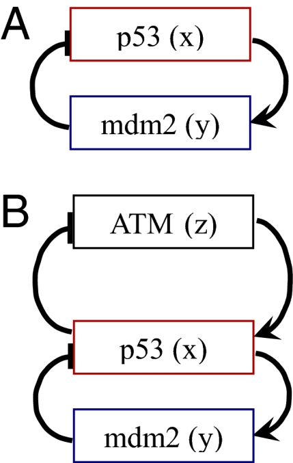
Schematic drawing of the p53 network. (A) Second-order equations: p53 (x) up-regulates mdm2 (y), which in turn inhibits p53. (B) The network based on the third-order model and its biological interpretation: The upstream factor ATM (z) is activated upon stress and activates p53 (x), which up-regulates mdm2 (y) and deactivates the signal (z). Mdm2 promotes the degradation of p53 and reduces its level. P53 inhibits ATM through the action of its downstream target wip1 (12, 14, 16).

To test the linearity of the present system, we applied a test commonly used in systems identification, based on the observation that linear differential equations with additive noise produce distributions that are Gaussian (35). We tested whether the experimental data for p53 and Mdm2 levels are distributed in a Gaussian manner, by measuring the ratio between the fourth and second central moments of the distribution across cells at each time point (kurtosis κ = < X⁴>/<X²>²). Gaussian distribution shows κ = 3 (compare with exponential distribution and gamma distributions with the same mean and STD as the present data showing κ ∼ 9). We find that the experimental protein level distributions have κ = 3.3 ± 0.7. The systems-identification linear model described below shows κ = 2.9 ± 0.2 when simulated on the same number of cells (Fig. S1). This supports the use of linear models for systems identification in the present case.

We began with a second-order model with two variables x = p53 and y = mdm2 (Fig. 4A), whose equations are

Here, N₁ and N₂ are noise terms that represent stochasticity in the reactions. In this model, we assume that the noise is white, meaning that it has no temporal correlations, and thus equally contains all frequencies. Below we consider also correlated noise.

We find that the best-fit model with two variables (x = p53 and y = Mdm2) captures the negative p53–mdm2 feedback loop interaction signs: Mdm2 (y) down-regulates p53 (x), a_xy = −0.8 ± 0.2 h⁻¹, and p53 (x) up-regulates mdm2 (y), a_yx = 0.8 ± 0.1 h⁻¹. However, this model does not capture the observed frequency behavior well. In particular, such a second-order model cannot show the increase in the experimental spectra observed at low frequencies (Fig. 3 A and B dashed line). In fact, one can connect the number of slope changes of the power spectrum with the minimal order of the underlying linear model: the observed power spectrum has at least three major slope changes (going down from zero frequency, then up to the main oscillation peak, then down again), and requires at least a third-order model.

We thus turned to a third-order model, in which we added a third variable z to represent ATM, the kinase that activates p53. In this model, ATM (z) has an interaction term with p53, with strength a_zx. We also allowed a term for the interaction back from p53 to ATM. The model equations are:

where a_ij are constants that represent interactions between the variables, and N₁, N₂, and N₃ are the noise of production of z, p53, and Mdm2, respectively.

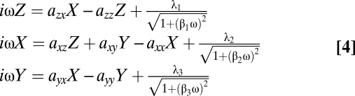
Fourier analysis transforms Eq. 2 into a set of coupled linear equations:

where ω is the frequency, Z(ω), X(ω), Y(ω) are the Fourier transforms of z, x, and y, respectively. λ₁, λ₂, and λ₃ are the Fourier transforms of the white noise N₁, N₂, and N₃, respectively (the Fourier transform of white noise is a constant).

Working with the Fourier transforms (Eq. 3) rather than the original differential equations (Eq. 2) has several well-known advantages: it allows handling noise in terms of constant terms, and it turns differential equations into algebraic ones, which are readily solvable.

We next fit the exact solution of Eq. 3 to the observed spectra. We find a single, well-defined best-fit solution, which is in agreement with the measured data (solid lines in Fig. 3). Note that there are no overfitting concerns in this case: the model has 10 free parameters, whereas the p53 and Mdm2 spectra have more than 10 relevant features. For example, the above-mentioned three slopes, together with the two corresponding turning point frequencies (the frequencies of the minimum and the resonance peak) make a total of 10 distinct features in the two power spectra that are captured by the model.

The best-fit parameters for the p53–Mdm2 interactions show the correct signs, and similar magnitudes, with activation of mdm2 by p53, a_yx = 0.29 ± 0.03 h⁻¹, and inhibition of p53 by Mdm2, a_xy = −0.55 ± 0.05 h⁻¹. The best-fit ATM–p53 interactions are two way, with ATM activating p53 and p53 inhibiting ATM. Such a feedback loop, with these signs, occurs in this system, where ATM is inhibited by a gene product of p53, WIP1 (12–14, 16). This feedback loop was experimentally and theoretically found to be important for oscillations (12). The strengths of these two interactions can be predicted in the best-fit model only up to their product a_xz × a_zx = −0.65 ± 0.05 h⁻².

Thus, this third-order model seems to capture current knowledge on the core of the p53 system that is needed for oscillations. Removing any of these interactions by setting their parameter to zero in the model significantly increases the fit error.

Analytical solution of the equations provides understanding of the way the power spectra increase at low frequencies. The analytical solution as ω → 0 scales as 1/ω² for p53 and as 1/ω for Mdm2, in agreement with the experimental spectra.

The best-fit noise amplitudes can also be estimated from the model, showing similar amplitudes for p53 and Mdm2: |λ₁/a_zx| = (1.4 ± 0.3) × 10³, λ₂ = (5 ± 1) × 10³, λ₃ = (10 ± 1) × 10³. The effective degradation rates of the proteins can also be estimated by the best-fit model: the p53 lifetime in the presence of Mdm2 in MCF7 cells as estimated by this approach is 75 ± 5 min, which is within a factor of two of the effective degradation rate found experimentally in WS1 cells (primary normal human skin fibroblasts) using immunoblots (36). The estimated lifetime of Mdm2 is 144 ± 10 min, four times longer than the experimentally measured lifetime in WS1 cells (36).

Stochastic simulation of the model equations (Eq. 2) in the time domain gives rise to sustained noisy oscillations reminiscent of the experimental data (Fig. 5 A and B). Without the white noise terms, this linear model would give only damped oscillations (Fig 5B, Inset). The oscillations are maintained by the noise, which continuously drives an otherwise stable third-order system.

Fig. 5.

Stochastic simulation shows sustained oscillations. (A and B) Shown are two runs of a stochastic simulation based on the set of differential equations (Eq. 2) using the best-fit parameters. The calculated p53 and Mdm2 profiles resemble the experimentally measured profiles. A deterministic simulation with the same parameters (but without noise) results in damped oscillations (Inset). (C and D) The experimental amplitude distribution of p53 (C) and Mdm2 (D), and a fit to a theoretical model of noise-driven damped harmonic oscillator (37) (solid lines).

The general features of oscillations driven by noise in a linear system were recently analyzed by Lang et al. (37). This analysis suggests that the distribution of peak amplitudes P(A) follows a distribution given by P(A) ∼ A × exp(−A²/A₀²). Here A is the peak amplitude and A₀ is given by the ratio of the noise strength and the protein degradation rate. We find that the measured peak distributions in our data are well described by this theoretical prediction (Fig. 5 C and D).

System Identification of p53–Mdm2 Oscillations Without DNA Damage Is Captured by a Second-Order Model.

We next applied the present approach to the dynamics of the p53 system without DNA damage. We reasoned that without damage, the ATM feedback loop should be inactive, and thus the system may be described by a second-order model (Fig. 3A) instead of a third-order model.

Our previous study (19) demonstrated that without DNA damage, p53 and Mdm2 oscillates at a frequency of ∼0.08 Hz (cycle time of ∼12 h). We performed Fourier analysis on the dynamics measured in that study and found a single peak at 0.08 Hz (Fig. 6). The power spectrum did not show the increase at low frequencies found in the spectrum with DNA damage (Fig. 3). As noted above, the single-peak shape of the spectrum suggests that a second-order linear set of equations may be sufficient to describe the dynamics. We indeed find that a second-order linear model (Eq. 1) describes the measured data very well (Fig. 6).

Fig. 6.

Fourier transforms of dynamics without DNA damage show a main peak, but not a rise at low frequencies. Shown is the RMS average over Fourier transforms of Mdm2–YFP levels. The measurement error was calculated as the SE of the individual Fourier transforms and is indicated by error bars. In this experiment, p53 dynamics were not measured. The calculated Fourier transform (solid line) is the solution of a second order Eq. 1 with parameters indicated in the text.

The second-order model provides well-defined best-fit estimates for all parameters, including interaction strengths, protein lifetimes, and noise amplitudes. The interaction strengths are a_xy = −0.73 ± 0.03 h⁻¹, a_yx = 0.34 ± 0.02 h⁻¹. The parameter describing the activation of mdm2 by p53 (a_yx) is equal (within the error range) to the one found with DNA damage. In contrast, the parameter that describes the degradation of p53 by mdm2 (a_xy) is lower than the one found with DNA damage. This implies that DNA damage in the present system enhances primarily the negative effect of mdm2 on p53 and does not measurably affect the activation of mdm2 by p53. The estimated lifetimes of p53 and mdm2 are 13 h and 180 min, respectively, which implies that the lifetime of p53 is considerably reduced following DNA breaks, whereas the lifetime of Mdm2 is almost uneffected. The noise parameters are λ₁ = (4 ± 1) × 10³, λ₂ = (6 ± 1) × 10³ and are on the same order as was found for the experiment with DNA damage.

Analysis of Exponentially Correlated Noise Suggests That the Best-Fit Noise Is Nearly Uncorrelated.

To further investigate the limits of the present model, we replaced the white noise in Eq. 2 with exponentially correlated noise. The correlation of this noise declines exponentially with time: <N(t)N(t + τ)> = λ²/β × e^−|τ|/β, where N is the noise, and β is the correlation decay time constant. White noise, which is uncorrelated, is a special limit of exponentially correlated noise with β → 0.

Applying exponential noise to the set of Eq. 2 gives the set of Fourier transforms:

where β_i are the decay time constants of the exponential noise terms. Note that as β_i approach zero one recovers the set of Eq. 3, in which the noise is white.

The set of Eq. 4 was solved analytically and fit to the experimental results. Again, one can estimate the system interaction parameters. The best-fit correlation decay coefficients β were all estimated as 2 ± 1 min, which means that the best-fit correlation time of the noise is very short and is practically zero. Thus, the nature of noise in the p53–Mdm2 model seems to be well approximated by uncorrelated white noise.

Discussion

We used a frequency-domain systems identification approach to analyze the p53–Mdm2 circuit in individual human cells. We find power spectra with a well-defined primary peak and a rise at low frequencies. This spectrum is well described by a third-order linear model with white noise (but not by a second-order model), with a factor upstream of p53 interpreted as ATM. The model identifies the negative feedback loop between ATM and p53, as well as the correct signs for the interactions in the p53–mdm2 negative feedback loop. It provides estimates for in vivo interaction strengths and noise amplitudes that are hard to otherwise measure and provides estimated in vivo life times for p53 and Mdm2 that are similar to previously measured values.

The model also captured the 12-h oscillations of the p53 system observed in the absence of DNA damage (19). In this case, a second-order model captures the spectra, which lack the low-frequency increase. This corresponds to the expectation that the upstream feedback loop with ATM should not be active in the absence of DNA damage.

The linear model constructed for this system can be considered as a linearization of a more general nonlinear dynamical system. Fourier analysis of the experimental oscillation traces shows several higher harmonics, suggesting the existence of nonlinear effects. However, a test of linearity suggests that the present system might be working reasonably close to its linear regime. Because of this near linearity, the present model supports a mechanism for sustained oscillations, in which noise drives an otherwise stable system by exciting frequencies close to its resonance frequency (37). It is of interest that this mechanism does not specifically require a delay between p53 and Mdm2. In contrast, delay is a required component in previously proposed nonlinear models that produce limit-cycle oscillations (19, 22, 28). It is useful to have two such qualitatively different classes of proposed mechanisms for p53 oscillations, because the two can potentially be differentially tested by experiments (e.g., by modulating the delay between p53 and Mdm2, for instance by placing Mdm2 under an early p53 responsive promoter).

This study used naturally occurring biological noise to effectively stimulate a wide range of frequencies in the system components. The noise is thus used as a natural diagnostic tool in the present approach (34). This complements the explicit introduction of oscillating or noisy inputs by experimentalists, as done in engineering and in biological applications (32, 38).

Fourier analysis of the p53–mdm2 allows identification of the circuit interactions by means of linear models. This approach is relatively noninvasive, because it relies on natural noise to stimulate the circuit at many frequencies at once. The suggested model estimates circuit characteristics that are otherwise hard to measure (noise amplitudes, in vivo interaction strengths, and protein lifetimes). This approach may be used to understand the behavior and the design of other cellular systems.

Materials and Methods

Cell Line and Constructs.

We used MCF7, human breast cancer epithelial cells, U280, stably transfected with pU265 and pU293 as described (18). In pU265, ECFP from pECFP-C1 (Clontech) was subcloned after the last codon of p53 cDNA, under the mouse metallothionein-1 promoter (MTΔ156) (39). This promoter provides a basal and constant level of transcription of p53–CFP. A basal promoter for p53–CFP was chosen because p53 is primarily regulated at the protein level and not at the transcriptional level (9). Control experiments with CFP expressed from this promoter showed constant expression with no oscillations. In pU293, the hMDM2 promoter was cloned by PCR using genomic DNA as a template, creating a 3.5-kb fragment upstream of the ATG site in exon 3, including P1 and P2 (40). This promoter was subcloned into pEYFP-1 (Clontech) (18).

Cells were maintained at 37 °C in RPMI medium 1640 containing 10% FCS (Sigma). To reduce background fluorescence, at 1–2 h before observation in the microscope, cells were grown in RPMI 1640 lacking riboflavin and phenol red (Biological Industries cat. no. 06–1100-26–1A), supplemented with l-glutamine, 10% FCS (certified FBS, membrane filtered; Biological Industries, 04–001-1A), and 0.05% penicillin-streptomycin antibiotics (Biological Industries, 03–031-1B). Cells were then exposed to the appropriate dose (10 Gy) of gamma irradiation (cesium source, 467 Gy h⁻¹). The number of DSBs has been found to be linear in gamma dose, with an average of about 30 DSB per Gy per cell (41).

Time-Lapse Microscopy.

Time-lapse movies were obtained at ×20 magnification in an automated inverted fluorescence microscope (DMIRE2 and DMI6000B; Leica). The microscope included live cell environmental incubators maintaining 37 °C (37-2 digital and heating unit, PeCon, Leica no. 15531719) humidity and 8% CO₂ (no. 0506.000–230; PeCon GmbH, Leica no. 11521733) and automated stage movement control (Corvus, ITK, GmbH); stage was surrounded by an enclosure to maintain constant temperature, CO₂ concentration, and humidity. Transmitted and fluorescence light paths were controlled by electronic shutters (Uniblitz, model VMM-D1); fluorescent light sources were mercury short arc lamp HXP and mercury HBO100 (OSRAM). Cooled CCD cameras were used: CoolSNAP, (Roper Scientific, photometrics), and ORCA-ER (C4742-95–12ERG, Hamamatsu photonics KK). Single-channel filters were from Chroma Technology, YFP: (500/20 nm excitation, 515 nm dichroic splitter, and 535/30 nm emission, Chroma no. 41028) and CFP: (436/20 nm, dichroic beam splitter 455 nm, emission 480/40 nm. The Leica system hardware was controlled by ImagePro5 Plus software (Media Cybernetics), which integrated time-lapse acquisition, stage movement, and software-based autofocus (adjusted in our lab).

Cells were grown and visualized in 12-well optical glass-bottom plates (MatTek cultureware, Microwell plates uncoated, part no. P12G-0–14-F, lot no. TK0289) coated with 10 μM fibronectin 0.1% (solution from bovine plasma, Sigma, cat. no. F1141) diluted 1:100 in Dulbecco's PBS, PBS (Sigma, cat. no. D8537). For each well, time-lapse movies were obtained at four fields of view. Each movie was taken at a time resolution of 20 min and was filmed for at least 2 d (over 140 time points). Each time point included transmitted light image (phase contrast) and two fluorescent channels (blue and yellow).

The mean cell generation time was about 20 h in the CO₂ incubated microscope without gamma irradiation. We find that movies using CFP and YFP illumination over 3 d did not visibly affect cell morphology or generation time.

Cell Tracking and Fluorescence Quantification.

Custom written image analysis software was developed using Matlab (Mathworks), which semiautomatically segmented and tracked individual cells. In each frame it automatically calculated the mean fluorescence intensity of pixels in the nucleus (after background subtraction) of CFP and YFP in individual cells. The main steps taken in each frame include: nuclei identification, tracking, and fluorescent intensity quantification.

Image background correction (flat field correction and background subtraction) was carried out as previously described (42). No significant bleaching was observed: on average bleaching was less than 3% over the duration of the experiment. Cellular autofluorescence of wild-type MCF7 cells without the CFP or YFP genes was negligible and gave consistent and low values with a mean of 25 CFP fluorescence units per pixel and 1 YFP fluorescence unit per pixel, with a coefficient of variation of ∼30%.

References

- 1.Tegner J, Yeung MK, Hasty J, Collins JJ. Reverse engineering gene networks: Integrating genetic perturbations with dynamical modeling. Proc Natl Acad Sci USA. 2003;100:5944–5949. doi: 10.1073/pnas.0933416100. [DOI] [PMC free article] [PubMed] [Google Scholar]
- 2.Mettetal JT, Muzzey D, Gómez-Uribe C, van Oudenaarden A. The frequency dependence of osmo-adaptation in Saccharomyces cerevisiae. Science. 2008;319:482–484. doi: 10.1126/science.1151582. [DOI] [PMC free article] [PubMed] [Google Scholar]
- 3.Lorenz DR, Cantor CR, Collins JJ. A network biology approach to aging in yeast. Proc Natl Acad Sci USA. 2009;106:1145–1150. doi: 10.1073/pnas.0812551106. [DOI] [PMC free article] [PubMed] [Google Scholar]
- 4.Alon U. An Introduction to Systems Biology: Design Principles of Biological Circuits. 1st Ed. The Netherlands: Chapman and Hall/CRC; 2006. Mathematical and Computational Biology Series. [Google Scholar]
- 5.Alon U. Network motifs: Theory and experimental approaches. Nat Rev Genet. 2007;8:450–461. doi: 10.1038/nrg2102. [DOI] [PubMed] [Google Scholar]
- 6.Santos SD, Verveer PJ, Bastiaens PI. Growth factor-induced MAPK network topology shapes Erk response determining PC-12 cell fate. Nat Cell Biol. 2007;9:324–330. doi: 10.1038/ncb1543. [DOI] [PubMed] [Google Scholar]
- 7.Momand J, Wu HH, Dasgupta G. MDM2—master regulator of the p53 tumor suppressor protein. Gene. 2000;242:15–29. doi: 10.1016/s0378-1119(99)00487-4. [DOI] [PubMed] [Google Scholar]
- 8.Prives C. Signaling to p53: Breaking the MDM2-p53 circuit. Cell. 1998;95:5–8. doi: 10.1016/s0092-8674(00)81774-2. [DOI] [PubMed] [Google Scholar]
- 9.Michael D, Oren M. The p53-Mdm2 module and the ubiquitin system. Semin Cancer Biol. 2003;13:49–58. doi: 10.1016/s1044-579x(02)00099-8. [DOI] [PubMed] [Google Scholar]
- 10.Harris SL, Levine AJ. The p53 pathway: Positive and negative feedback loops. Oncogene. 2005;24:2899–2908. doi: 10.1038/sj.onc.1208615. [DOI] [PubMed] [Google Scholar]
- 11.Shiloh Y. ATM and related protein kinases: Safeguarding genome integrity. Nat Rev Cancer. 2003;3:155–168. doi: 10.1038/nrc1011. [DOI] [PubMed] [Google Scholar]
- 12.Batchelor E, Mock CS, Bhan I, Loewer A, Lahav G. Recurrent initiation: A mechanism for triggering p53 pulses in response to DNA damage. Mol Cell. 2008;30:277–289. doi: 10.1016/j.molcel.2008.03.016. [DOI] [PMC free article] [PubMed] [Google Scholar]
- 13.Lu X, Nannenga B, Donehower LA. PPM1D dephosphorylates Chk1 and p53 and abrogates cell cycle checkpoints. Genes Dev. 2005;19:1162–1174. doi: 10.1101/gad.1291305. [DOI] [PMC free article] [PubMed] [Google Scholar]
- 14.Fiscella M, et al. Wip1, a novel human protein phosphatase that is induced in response to ionizing radiation in a p53-dependent manner. Proc Natl Acad Sci USA. 1997;94:6048–6053. doi: 10.1073/pnas.94.12.6048. [DOI] [PMC free article] [PubMed] [Google Scholar]
- 15.Fujimoto H, et al. Regulation of the antioncogenic Chk2 kinase by the oncogenic Wip1 phosphatase. Cell Death Differ. 2006;13:1170–1180. doi: 10.1038/sj.cdd.4401801. [DOI] [PubMed] [Google Scholar]
- 16.Shreeram S, et al. Wip1 phosphatase modulates ATM-dependent signaling pathways. Mol Cell. 2006;23:757–764. doi: 10.1016/j.molcel.2006.07.010. [DOI] [PubMed] [Google Scholar]
- 17.Lev Bar-Or R, et al. Generation of oscillations by the p53-Mdm2 feedback loop: A theoretical and experimental study. Proc Natl Acad Sci USA. 2000;97:11250–11255. doi: 10.1073/pnas.210171597. [DOI] [PMC free article] [PubMed] [Google Scholar]
- 18.Lahav G, et al. Dynamics of the p53-Mdm2 feedback loop in individual cells. Nat Genet. 2004;36:147–150. doi: 10.1038/ng1293. [DOI] [PubMed] [Google Scholar]
- 19.Geva-Zatorsky N, et al. Oscillations and variability in the p53 system. Mol Syst Biol. 2006;2 doi: 10.1038/msb4100068. 2006.0033. [DOI] [PMC free article] [PubMed] [Google Scholar]
- 20.Hamstra DA, et al. Real-time evaluation of p53 oscillatory behavior in vivo using bioluminescent imaging. Cancer Res. 2006;66:7482–7489. doi: 10.1158/0008-5472.CAN-06-1405. [DOI] [PubMed] [Google Scholar]
- 21.Hoffmann A, Levchenko A, Scott ML, Baltimore D. The IkappaB-NF-kappaB signaling module: Temporal control and selective gene activation. Science. 2002;298:1241–1245. doi: 10.1126/science.1071914. [DOI] [PubMed] [Google Scholar]
- 22.Tiana G, Krishna S, Pigolotti S, Jensen MH, Sneppen K. Oscillations and temporal signalling in cells. Phys Biol. 2007;4:R1–R17. doi: 10.1088/1478-3975/4/2/R01. [DOI] [PubMed] [Google Scholar]
- 23.Monk NA. Oscillatory expression of Hes1, p53, and NF-kappaB driven by transcriptional time delays. Curr Biol. 2003;13:1409–1413. doi: 10.1016/s0960-9822(03)00494-9. [DOI] [PubMed] [Google Scholar]
- 24.Tyson JJ, Chen KC, Novak B. Sniffers, buzzers, toggles and blinkers: Dynamics of regulatory and signaling pathways in the cell. Curr Opin Cell Biol. 2003;15:221–231. doi: 10.1016/s0955-0674(03)00017-6. [DOI] [PubMed] [Google Scholar]
- 25.Nelson DE, et al. Oscillations in NF-kappaB signaling control the dynamics of gene expression. Science. 2004;306:704–708. doi: 10.1126/science.1099962. [DOI] [PubMed] [Google Scholar]
- 26.Tyson JJ. Monitoring p53’s pulse. Nat Genet. 2004;36:113–114. doi: 10.1038/ng0204-113. [DOI] [PubMed] [Google Scholar]
- 27.Ciliberto A, Novak B, Tyson JJ. Steady states and oscillations in the p53/Mdm2 network. Cell Cycle. 2005;4:488–493. doi: 10.4161/cc.4.3.1548. [DOI] [PubMed] [Google Scholar]
- 28.Ma L, et al. A plausible model for the digital response of p53 to DNA damage. Proc Natl Acad Sci USA. 2005;102:14266–14271. doi: 10.1073/pnas.0501352102. [DOI] [PMC free article] [PubMed] [Google Scholar]
- 29.Oppenheim AV, Willsky AS, Young IT. Signal and Systems. Englewood Cliffs, NJ: Prentice-Hall; 1983. [Google Scholar]
- 30.Bode HW. Network Analysis and Feedback Amplifier Design. New York: Van Nostrand; 1955. [Google Scholar]
- 31.Graupe D. Identification of Systems. New York: Van Nostrand Reinhold; 1972. [Google Scholar]
- 32.Block SM, Segall JE, Berg HC. Impulse responses in bacterial chemotaxis. Cell. 1982;31:215–226. doi: 10.1016/0092-8674(82)90421-4. [DOI] [PubMed] [Google Scholar]
- 33.Taylor RJ, et al. Dynamic analysis of MAPK signaling using a high-throughput microfluidic single-cell imaging platform. Proc Natl Acad Sci USA. 2009;106:3758–3763. doi: 10.1073/pnas.0813416106. [DOI] [PMC free article] [PubMed] [Google Scholar]
- 34.Dunlop MJ, Cox RS, 3rd, Levine JH, Murray RM, Elowitz MB. Regulatory activity revealed by dynamic correlations in gene expression noise. Nat Genet. 2008;40:1493–1498. doi: 10.1038/ng.281. [DOI] [PMC free article] [PubMed] [Google Scholar]
- 35.Kloeden PE, Platen E. Numerical Solution of Stochastic Differential Equations. Berlin: Springer; 1999. [Google Scholar]
- 36.Stommel JM, Wahl GM. Accelerated MDM2 auto-degradation induced by DNA-damage kinases is required for p53 activation. EMBO J. 2004;23:1547–1556. doi: 10.1038/sj.emboj.7600145. [DOI] [PMC free article] [PubMed] [Google Scholar]
- 37.Lang M, Waldherr S, Allgöwer F. Amplitude distribution of stochastic oscillations in biochemical networks due to intrinsic noise. PMC Biophys. 2009;2:10. doi: 10.1186/1757-5036-2-10. [DOI] [PMC free article] [PubMed] [Google Scholar]
- 38.Pedraza JM, Oudenaarden Av. Complex Systems Science in BioMedicine. New York: Kluwer Academic; 2006. [Google Scholar]
- 39.Brinster RL, Chen HY, Warren R, Sarthy A, Palmiter RD. Regulation of metallothionein—thymidine kinase fusion plasmids injected into mouse eggs. Nature. 1982;296:39–42. doi: 10.1038/296039a0. [DOI] [PubMed] [Google Scholar]
- 40.Oliner JD, Kinzler KW, Meltzer PS, George DL, Vogelstein B. Amplification of a gene encoding a p53-associated protein in human sarcomas. Nature. 1992;358:80–83. doi: 10.1038/358080a0. [DOI] [PubMed] [Google Scholar]
- 41.Bonner WM. Low-dose radiation: Thresholds, bystander effects, and adaptive responses. Proc Natl Acad Sci USA. 2003;100:4973–4975. doi: 10.1073/pnas.1031538100. [DOI] [PMC free article] [PubMed] [Google Scholar]
- 42.Sigal A, et al. Variability and memory of protein levels in human cells. Nature. 2006;444:643–646. doi: 10.1038/nature05316. [DOI] [PubMed] [Google Scholar]
Associated Data
This section collects any data citations, data availability statements, or supplementary materials included in this article.