Semi-supervised recursively partitioned mixture models for identifying cancer subtypes

Abstract

Motivation: Patients with identical cancer diagnoses often progress differently. The disparity we see in disease progression and treatment response can be attributed to the idea that two histologically similar cancers may be completely different diseases on the molecular level. Methods for identifying cancer subtypes associated with patient survival have the capacity to be powerful instruments for understanding the biochemical processes that underlie disease progression as well as providing an initial step toward more personalized therapy for cancer patients. We propose a method called semi-supervised recursively partitioned mixture models (SS-RPMM) that utilizes array-based genetic and patient-level clinical data for finding cancer subtypes that are associated with patient survival.

Results: In the proposed SS-RPMM, cancer subtypes are identified using a selected subset of genes that are associated with survival time. Since survival information is used in the gene selection step, this method is semi-supervised. Unlike other semi-supervised clustering classification methods, SS-RPMM does not require specification of the number of cancer subtypes, which is often unknown. In a simulation study, our proposed method compared favorably with other competing semi-supervised methods, including: semi-supervised clustering and supervised principal components analysis. Furthermore, an analysis of mesothelioma cancer data using SS-RPMM, revealed at least two distinct methylation profiles that are informative for survival.

Availability: The analyses implemented in this article were carried out using R (http://www.r.project.org/).

Contact: devin_koestler@brown.edu; e_andres_houseman@brown.edu

Supplementary information: Supplementary data are available at Bioinformatics online.

1 INTRODUCTION

There are approximately 200 known types of cancer, although they may be overly general as the same type of cancer can have very different trajectories in different people. For example, it is not unusual for a tumor to proliferate in one patient and stabilize or regress in another, even though their tumors are indistinguishable at a microscopic level. Traditionally, researchers diagnosed and treated cancer based on an analysis of cell shape and size, a method that is substantially challenging for closely related cancers. In recent years, information regarding molecular alterations in cancer has contributed to defining cancer subtypes based on the underlying molecular signature of a tumor (Alizadeh et al., 2000; Lapointe et al., 2004; Sorlie et al., 2003). Such molecular pathology has contributed to the discovery of subtypes of several different tumor types and has successfully identified patients with different survival times (Beer et al., 2002; van de Vijver et al., 2002; van't Veer et al., 2002). More recently, there has been substantial interest in the use of methylation profiling for understanding the effect of epigenetic alterations on disease susceptibility as well as to characterize cancer subtypes based on methylation patterns (Ang et al., 2010; Christensen et al., 2009b, c; Deneberg et al., 2010; Marsit et al., 2009). However, such associations work best when cancer subtypes based on genetic profiles are already known. If subtype membership is known, then a number of different supervised classification procedures such as support vector machines (SVMs), discriminant analysis, multinomial logistic regression or ensemble-based procedures, can be used to build a statistical model to diagnose such cancers in future patients. In most instances, however, neither the different subtypes nor patient-specific subtypes are known. Consequently, attempts have been made to identify cancer subtypes, many of which use either fully unsupervised learning or fully supervised learning techniques. Unsupervised analyses for identifying cancer subtypes is often addressed using hierarchical clustering (Eisen et al., 1998), where cancer subtypes are identified using only array-based genetic data. As Bair and Tibshirani (2004) report, hierarchical clustering can be an effective method for identifying clinically relevant cancer subtypes, although one major limitation of unsupervised learning procedures is that they may identify cancer subtypes that are unrelated to patient survival or other clinical outcomes of interest, especially when they are applied to high-dimensional data. Since unsupervised learning procedures use no clinical data for identifying cancer subtypes, there is no guarantee that identified subtypes will strongly predict outcome. An alternative approach to identifying subtypes is the use of a supervised learning algorithm that explicitly models survival. However, such approaches often result in models with limited biological interpretation.

To overcome the limitations of fully unsupervised and fully supervised approaches, Bair and Tibshirani (2004) proposed a procedure known as semi-supervised clustering (SS-Clust), which combines both gene expression data and clinical data to identify cancer subtypes. First, their procedure identifies a set of genes that correlate with the clinical variable of interest, then subsequently applies an unsupervised clustering technique to that set of genes, forming a prediction rule for cluster assignment. Several variants of this procedure have been proposed, in particular, supervised principal components analysis (SPCA). Unlike SS-Clust, SPCA computes a ‘risk score’ for each patient which is subsequently used as a continuous predictor of survival. The semi-supervised methods of Bair and Tibshirani (2004), specifically, SS-Clust and SPCA, have been used in number of studies for identifying biologically meaningful cancer subtypes as well as for predicting patient survival (Bullinger et al., 2004; Hou et al., 2010; Jiang et al., 2008; Yu et al., 2008; Zhao et al., 2006). Although both procedures have proven to be successful strategies, they have a number of limitations. In particular, the performance of SS-Clust is compromised when the number of clusters is misspecified, specifically in situations in which there are a large number of subgroups that have considerable overlap. Moreover, SPCA does not facilitate the attainment of discrete cancer subtypes, which are often of clinical interest, and inherits the interpretability issues inherent to PCA. To this end, we propose a semi-supervised approach, which is similar in spirit to the semi-supervised strategies of Bair and Tibshirani (2004); however, we substitute use of PCA or other latent variable methods with the use of recursively partitioned mixture models (RPMM; Houseman et al., 2008). RPMM is a model-based hierarchical clustering method that estimates the number of clusters and produces a reliable solution in a shorter time than the standard finite mixture model approach with sequential mixture model fitting attempts using different numbers of assumed clusters.

The remainder of this article is organized as follows: in Section 3, we provide overviews of both RPMM and the Bair and Tibshirani (2004) SS-Clust approach and propose a semi-supervised version of RPMM. In Section 4, we present simulation results and in Section 5 we demonstrate our method on a mesothelioma cancer dataset. We follow with a discussion and conclusion in Sections 6 and 7.

2 BACKGROUND

A challenge in clustering problems is the selection of the number of clusters K (Chen, 1995). Since inference post-clustering is heavily influenced by the choice K, misspecification of the number of clusters often leads to misleading or erroneous results. Hence, reliable and robust methods for choosing K are necessary. Bayesian solutions to clustering exist (Tadesse et al., 2005) but are computationally demanding. Computationally efficient, scalable methods are necessary for routine bioinformatics and molecular biology research. Houseman et al. (2008) proposed RPMM, an unsupervised method for model-based clustering of data, which presents the number of clusters and a dependable solution in a shorter amount of time than repeated attempts with different numbers of assumed clusters. The initial description of RPMM in Houseman et al. (2008) assumed beta-distributed responses, however, in general, any parametric distribution (univariate or multivariate) can be used, and for mRNA or miRNA expression data, a Gaussian response may be more appropriate.

RPMM is similar to the idea of recursive partitioning with subsequent tree pruning used in hierarchical ordered partitioning and collapsing hybrid (HOPACH; van der Laan and Pollard, 2003), in which clusters are recursively partitioned using a non-parametric algorithm such as partitioning around medoids (PAMs; Kaufman and Rousseeuw, 1990). However, Houseman et al. (2008) show that the model-based construction of RPMM can result in superior results.

3 STATISTICAL METHODS

3.1 Overview of RPMM

The reader may refer to Houseman et al. (2008) for a comprehensive description of RPMM. For each single subject i, we assume class membership C_i ∈ {1, 2,…, K}. For assay data Y_ij from subject i ∈ {1, 2,…, n} at gene or locus j ∈ {1, 2,…, J}, we assume the distribution f(Y_ij = y|C_i = k; θ_kj) , where θ_kj is a vector of parameters that depends on both class k and locus j. Houseman et al. (2008) assumed beta-distributed responses, although in general any parametric distribution can be used. Under the assumption that C_i = k with probability η_k, where ∑_k=1^K η_k = 1, and that expression of each gene is independent conditional on class membership, the likelihood contribution from subject i is given by

where ς = (η₁,…, η_K−1, θ₁₁,…, θ_1J, θ₂₁,…,θ_KJ) is a vector of parameters. With observed data 𝒟 = {y₁, y₂,…, y_n}, the conventional mixture model approach involves maximizing the full-data log-likelihood,

(1)

with respect to ς. This is easily achieved using an Expectation-Maximization (EM) algorithm (Dempster et al., 1977). Briefly, we initialize the procedure with an n × K matrix of weights W = (w_ik) whose rows sum to one. The rows represent initial guesses at class membership probabilities for each subject. For each k, we maximize the quantity

(2)

to obtain estimates of the parameters corresponding to class k. Reversing the order of summation in (2) shows that each dimension j can be maximized separately. We subsequently update the weights as follows:

(3)

iterating the maximization of (2) and recalculation of (3) until ℓ(ς) stays fixed. The final weight w_ik represents the posterior probability that subject i belongs to class k [i.e. w_ik = P(C_i = k|Y₁,…, Y_n, ς)]. Since the number of classes K is typically unknown, we might decide on the number of classes by fitting mixture models for a range of possible values of K, computing the Bayesian Information Criterion (BIC) statistic 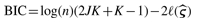and selecting the value of K that corresponds to the minimum BIC. The entire operation has approximate complexity nJK_max², where K_max is the maximum number of classes attempted.

Houseman et al. (2008) proposed a recursive alternative that has complexity no more than nJK log K. Consider the following weighted-likelihood version of (1),

(4)

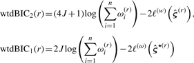
When ω_i ≡ 1 for all i, (1) and (4) are equivalent. When 0 < ω_i < 1, subject i only partially contributes to estimation, and when ω_i = 0, subject i is excluded entirely from consideration. The EM algorithm described above is easily modified by substituting each w_ik with ω_iw_ik in (2), where the interpretation is that the classes under consideration are only a partial set, and that subject i belongs to one of these classes only with probability ω_i. Thus, the procedure begins by fitting a two-class model to the entire dataset, where the result is two sets of posterior weights representing the posterior probabilities of membership in each of the two classes. Under the assumption that each of these classes can be further split, and that each subject belongs to the subsequent splits only with probability equal to the weight assigned to the unsplit class, the weighted-likelihood EM algorithm is applied to obtain the two classes corresponding to the new split. If the EM algorithm fails due to insufficient data, then recursion is terminated at that point. However, if the EM algorithm succeeds, new weights are established and recursion is continued. As mentioned in Houseman et al. (2008), at each level of recursion, the weights become smaller; since a mixture model becomes unstable with small weights (corresponding to small numbers of pseudo-subjects), the recursion ultimately terminates completely at a set of terminal or leaf nodes corresponding to unsplit classes. This process is stabilized by terminating the recursion if the sum of the weights is less than some prespecified value (e.g. 5). Additionally, recursion can be terminated early if the split leads to a less parsimonious representation of the data. Houseman et al. (2008) propose using the BIC, to motivate a criterion for rejecting a proposed split. In particular, they proposed the following weighted versions of BIC:

(5)

where the first vector of parameters, defining wtdBIC₂(r), is obtained from the two-class mixture model and the second vector of parameters, defining wtdBIC₁(r), is obtained from a one-class model. Note, the effective sample size is considered to be ∑_i=1ⁿ ω_i^(r). If wtdBIC₂(r) is greater than wtdBIC₁(r), the recursion is terminated at node r. After all nodes terminate, the solution to the clustering problem consists of K classes, with the final assembled from the individual vectors θ_kj and the prevalence estimates , where ω_i^(r) represents the class probability for subject i for a recursion sequence r.

Houseman et al. (2008) studied the properties of RPMM via simulation on realistic datasets motivated by DNA methylation data on normal tissues and found that RPMM and conventional model-based clustering (e.g. sequential mixture model fitting with K selected via BIC) had similarly superior clustering performance relative to several non-parametric alternatives, including HOPACH (van der Laan and Pollard, 2003) and dynamic tree cutting (Langfelder et al., 2008), but that RPMM was much faster than sequential mixture model fitting with different number of assumed classes.

3.2 SS-Clust

Suppose our data consists of n samples on J molecular loci and we assume that there are several distinct molecular classes relevant to a clinical outcome. In keeping with Bair and Tibshirani (2004), we a assume a survival outcome, although a simpler outcome (e.g. binary) could be used as well. The Bair and Tibshirani (2004) procedure begins by selecting the M ≪ J genes that are most associated with survival. This can be accomplished by fitting J Cox-proportional hazards models (one for each of the J genes) and computing the Cox-scores (i.e. values of where represents the proportional hazards estimate of the log-hazard ratio for the j-th gene). In short, the Cox-score is a measure of the association between the gene's expression level and patient survival. Using the M genes with the largest absolute Cox-scores, where M is typically chosen based on cross-validation, K-means clustering is applied to n observations. Based on the K-means clustering results, the n observations are then assigned putative class labels. As described in Bair and Tibshirani (2004), the choice of K for K-means clustering is typically chosen based on prior biological knowledge, although they assert that K = 2 generally works well for most datasets. Using the class label assignments for the n observations based on K-means clustering, the n samples and all J loci are then used to train a nearest shrunken centroid (NSC) classifier (Tibshirani et al., 2003). One can then use the NSC classifier to assign future patients to one of the K subgroups. Compared with competing methodologies, SS-Clust tends to perform very well with respect to predicting survival and has the distinct advantage of reducing the effective number of J genes used for clustering and classification.

In addition to selecting a subset of genes based on the largest absolute Cox-scores, Bair and Tibshirani (2004) also propose selecting a subset of genes using partial least squares (PLS) to compute corrected Cox-scores. As described, selecting the genes with the largest absolute corrected Cox-scores, in some instances, produces better clusters than selecting genes with the largest raw Cox-scores.

3.3 Semi-supervised RPMM

While SS-clust is an extremely successful strategy, it requires knowledge of the number of underlying clusters, and does not perform well when this number is misspecified, specifically in situations where there are a large number of overlapping classes (Bair and Tibshirani, 2004). Since RPMM is able to estimate the number of clusters in a robust and computationally efficient manner, we propose a semi-supervised RPMM (SS-RPMM) approach, which is similar in spirit to that proposed by Bair and Tibshirani (2004), but with substitution of LCA, PCA or any other latent variable method, by RPMM.

We assume that classification of a random variable Z is of interest. This variable could be a Gaussian response or a binary response, but in this article we focus on a survival response, both because survival was the focus of Bair and Tibshirani (2004), and because it represents a relatively complicated datatype. We assume a proportional hazards model,

(6)

where X_i represents any additionally relevant patient-specific information and 𝕀(C_i = k) is an indicator of class membership in the k-th class for the i-th patient. We take Z_i = (T_i, d_i), where T is the observed failure or censoring time and d is an indicator of whether or not the event was observed. As in Bair and Tibshirani (2004), we first fit univariate (e.g. single locus models) Cox models of the form

(7)

where Y_ij represents the expression of gene j in subject i. Fixing M, we take the set 𝒥_M^⋆ of the M genes j having the M largest Cox-scores, either raw or PLS Cox-scores. We then fit an RPMM model to the genes represented by 𝒥_M^⋆; the resulting model provides the latent class structure on the preselected genes. We then use the latent class assignments to fit (6). Since the RPMM class assignments are based on posterior class membership probabilities , we can either assign classes based on the highest posterior membership probability, or else use a weighted Cox model [e.g. as in Houseman et al. (2006)], to obtain an approximate solution where there are a large number of imperfectly classified subjects.

Assuming the dataset 𝒟 can be split randomly into a training set 𝒟₀ and a test set 𝒟₁, we perform the preselection procedure on 𝒟₀, followed by RPMM on 𝒟₀ using the M preselected genes. Using the RPMM solution from 𝒟₀, we construct empirical Bayes estimates Ĉ_i of class assignments on the test set 𝒟₁ and assign subjects to the class that has the largest predicted posterior probability, . We subsequently fit (6) to 𝒟₁ using the class assignments Ĉ_i. We can then assess the prediction performance using pseudo R² (Schemper, 1990). Since M is a tuning parameter, it should be selected with care. As in Bair and Tibshirani (2004), M can be determined using cross-validation. Table 1 presents a variant of this algorithm.

Table 1.

Algorithm for determining M, the number of preselected genes with the largest absolute Cox-score to be used in fitting RPMM

(1) Randomly split the Training set 𝒟0 into two sets: 𝒟0a and 𝒟0b. (2) Fit RPMM to 𝒟0a using the M preselected genes with largest absolute Cox-scores. (3) Using the results from the RPMM fit on 𝒟0a, predict class membership Ĉi for the observations in 𝒟0b using empirical Bayes and assign the observations in 𝒟0b to the class which has the largest posterior probability. (4) Compute and record the P-value for the log-rank test, testing the hypothesis that the hazard of dying is the same for each of the predicted classes in 𝒟0b. (5) Repeat steps 2–4 varying M from Mmin to Mmax, where Mmin and Mmax are thresholds selected by the user. (6) Repeat steps 1–5 making different splits of 𝒟0 into 𝒟0a and 𝒟0b. (7) Compute the median P-value for each specification of M across the different splits of 𝒟0. (8) Set M = M⋆, where M⋆ is the specification of M that results in the smallest median P-value.

4 IMPLEMENTATION

We conducted simulations to compare both SS-Clust and SPCA to SS-RPMM. The simulated datasets were generated in a similar way to that described in Bair and Tibshirani (2004). Training and testing datasets each consisted of 3000 gene expression measurements for 250 samples, which were distributed among five classes each of which contained 50 samples. For the first class, genes 1–50 were generated from a normal distribution with mean 0.25 and SD 0.15; for the second class, genes 1–50 were generated from a normal distribution with mean 0.40 and SD 0.15; for the third class, genes 1–50 were generated from a normal distribution with mean 0.55 and SD 0.15; for the fourth class, genes 1–50 were generated from a normal distribution with mean 0.70 and SD 0.15; and for the fifth class, genes 1–50 were generated from a normal distribution with mean 0.85 and SD 0.15. As in Bair and Tibshirani (2004), we introduced several additional genes which were unrelated to the clinical variable of interest; we randomly selected 40% of the samples to have a mean of 0.4 and SD of 0.15 for genes 51–250; 50% of the samples to have a mean 0.5 and SD 0.15 for genes 251–450; and 70% of the samples to have a mean 0.7 and SD 0.15 for genes 451–650. The other 60, 50 and 30% of samples for genes 51–250, 251–450 and 451–650, respectively, were sampled from a normal distribution with mean 0 and SD 0.35. Additionally, the remaining genes 651–3000, were generated from a normal distribution with mean 0 and SD 0.35 for each of the 250 samples.

The survival times for the first class were generated from a normal distribution with mean 30 and SD 4; for the second class survival times were generated from a normal distribution with mean 33 and SD 4; for the third class, survival times were generated from a normal distribution with mean 36 and SD 4; for the fourth class, survival times were generated from a normal distribution with mean 39 and SD 4; and for the fifth class, survival times were generated from a normal distribution with mean 42 and SD 4. For each of the 250 samples, the survival times were assumed to have been observed, thus censoring was not present in our simulations.

For each method, PLS Cox-scores were calculated to assess the association between gene expression across samples and the clinical variable of interest, which in our simulations was survival time. Since there were 50 genes that differentiated between classes with respect to survival time, we investigated several choices for M, M ∈ {15, 25, 50, 75}, the number of genes selected on the basis of the largest PLS Cox-score. Furthermore, we also considered several different choices for the number of assumed clusters K, K ∈ {2, 3, 4, 5, 6} to be used in the K-means clustering step of the SS-Clust algorithm. There is no dependency on the value of K assumed for the SS-RPMM and SPCA approaches. We considered 100 simulations for each level of M and K. Under the SS-Clust framework, class memberships for the observations in the testing data were determined by fitting a NSC classifier on the training data using the putative class labels assigned via K-means clustering and applying this classifier to testing data to obtain class memberships for each observation. Similarly, under the SS-RPMM framework, class memberships for the observations in the testing data were determined by fitting a normally distributed RPMM on the training data, followed by empirical Bayes using the obtained parameter estimates, which provided posterior probabilities of class membership for each class for each observation in the testing data. Each observation in the testing data was then assigned to the class for which the posterior class membership probability was the highest. For the SPCA procedure, PCA was implemented on the training data using only the M genes with the largest absolute PLS Cox-scores. The resulting solution was used to approximate the principal components for the testing data. We used the Rand Index (Rand, 1971), which provides a measure of similarity between the true class membership and the predicted class membership, to assess how SS-RPMM compared with SS-Clust in terms of correctly classifying the observations in the testing data. Additionally, we used pseudo-R² to assess the predictive ability of SS-RPMM, SS-Clust and SPCA. For SS-RPMM and SS-Clust, the pseudo-R² was calculated by fitting a Cox-proportional hazards model to the testing data, using the predicted class memberships as factors in the model. For SPCA, the pseudo-R² was calculated by fitting a Cox-proportional hazards model to the testing data using the approximated principal components.

The average Rand Index was compared between the SS-Clust and SS-RPMM methods across the different settings of M and K, Supplementary Figure S1. For a fixed M, the average Rand Index obtained for the SS-Clust approach tended to increase as the number of assumed clusters K increased toward the true number of classes. Moreover, for a fixed K, the average Rand Index for both SS-Clust and SS-RPMM, tended to be higher as M was increased toward the true number of genes that differentiated between classes relative to survival. Similar trends were seen with respect to the average pseudo-R², Figure 1. Most notably, however, SS-RPMM and SPCA(2) had comparable performance with SS-RPMM having a slightly larger average pseudo-R² for each M among the three methods.

Fig. 1.

Average pseudo-R² between SS-RPMM, SS-Clust, SPCA using the first principal component only SPCA(1), and using the first and second principal components SPCA(2), for different settings of M and K. Results are based on 100 simulations.

The results from this simulation study show that, with respect to classification performance, SS-RPMM tends to outperform SS-Clust, the extent to which depended on the degree of misspecification of the number of assumed clusters K. Moreover, SS-RPMM explained more variability in survival compared with SS-Clust and explained a similar amount of variability compared with SPCA. A number of additional simulations were implemented to access the classification and prediction performance of SS-RPMM relative to SS-Clust and SPCA under model misspecification. We evaluated the performance of the three methods where the genetic data for the training and testing sets were sampled from a t-distribution with low degrees of freedom and a normally distributed RPMM was assumed (Supplementary Figs S3–S4). Since RPMM assumes class conditional independence of genes/loci, we also implemented a simulation study comparing the classification and prediction performance of the three methods where we imposed within-class correlation between genes (Supplementary Figs S5–S8). The full description and results of these simulations are provided in the Supplementary Material. Briefly, however, SS-RPMM outperformed SS-Clust with respect to both classification and prediction performance and had similar performance compared with SPCA in terms of prediction performance. In the presence of within-class correlation, RPMM tended to overestimate the number of classes; this phenomenon is similar to that found by Lindsay et al. (1991).

We also considered a simulation study where M was selected based on cross-validation (Supplementary Table S1). The description and results of this simulation study can be found in the Supplementary Material. Briefly, the results of this simulation study showed better prediction and classification performance of SS-RPMM over SS-Clust and similar prediction performance between SS-RPMM and SPCA. Lastly, we implemented a simulation study where we used a modified version of the SS-Clust algorithm. Specifically, instead of fitting the NSC using all genes, we used only those M genes that were used in the K-means clustering step. The results of this simulation are provided in Supplementary Figure S9 and show that, with respect to Rand Index and pseudo-R², SS-RPMM and SS-Clust tended to perform similarly when the number of assumed clusters K was correctly specified, with SS-Clust performing slightly better than SS-RPMM. This is likely due to the fact that SS-RPMM incurs a cost for estimating K, while SS-Clust receives the benefit of having K ‘known’. Similar to our previous simulations, however, when K was misspecified, SS-RPMM tended to outperform SS-Clust, the magnitude to which depended on the degree of misspecification.

As demonstrated in our simulations, SS-RPMM tended to outperform SS-Clust with respect to survival prediction and classification performance. Furthermore, the prediction performance was comparable between SS-RPMM and SPCA. Although RPMM relies on distributional assumptions and class conditional independence, additional simulation studies have indicated favorable performance of SS-RPMM over SS-Clust and SPCA even when these assumptions are violated (Supplementary Figs S3–S8).

5 MESOTHELIOMA CANCER EXAMPLE

The mesothelioma dataset consisted of 158 tumor samples derived from two, independent series of mesothelioma cases (Christensen et al., 2009c). The aim of this study was to identify risk factors associated with an increased mortality from mesothelioma.

Each of the 158 tumor samples were profiled for the methylation status at 1505 CpG loci associated with 803 cancer-related genes simultaneously using the Illumina GoldenGate® methylation bead arrays. Sample preparation has been described previously (Christensen et al., 2009a, c). As discussed in Houseman et al. (2008), the result of the array is a sequence of ‘beta’ values between zero and one, one for each of the 1505 CpG loci. A total of 1497 passed QA/QC procedures (median detection P < 0.05), and of these, 1413 autosomal loci were used in subsequent analysis. In addition to methylation profiles for each of the 1505 CpG loci, the mesothelioma dataset consists of information on time to death after diagnosis, as well as various demographic and clinical covariates. Among the 158 samples, there were 107 deaths with a median survival time of 17 months. The full dataset was used to generate training (N₀ = 79) and testing (N₁ = 79) sets. Training and testing sets were obtained by randomly sampling within tumor histology. There were no significant differences between the training and testing sets with respect to relevant covariates (e.g. gender, smoking status, age, etc.) Furthermore, there was no significant difference between the training and testing sets with respect to survival (log-rank test P = 0.862). The training data were used to identify CpG loci that are associated with survival time. A series of Cox-proportional hazards models, stratified by tumor histology and controlling for age and gender, were fit for each of the 1413 loci. Using the R package (http://www.r.project.org/) RPMM version 1.05, a RPMM assuming beta distributed responses, was fit to the training set using the M CpG loci with the largest absolute Cox-scores, where M was determined using the algorithm described in Table 1. After fitting RPMM to the training data using the M CpG loci with the largest Cox-scores, we used the model to predict class membership for each observation in the testing set by assigning the class with the largest posterior probability. To determine whether the predicted classes in the testing set were associated with survival, we fit a Cox-proportional hazards model stratified by tumor histology controlling for age and gender, where predicted class membership in testing set was treated as a factor. Using the nested cross-validation procedure described in Table 1, we determined that M = 41. Subsequently, fitting RPMM to the training data using the 41 CpG loci with the largest absolute Cox-scores resulted in three classes.

There were 36 observations assigned to class L, 22 observations assigned to class RL, and 21 observations assigned to class RR. The results obtained from fitting a Cox-proportional hazards model to the testing data are given in Table 2. Class RR had a significantly lower hazard of dying (95 % CI for the hazard ratio; [0.17,0.73]), compared with class L. Class RL did not have a significantly different hazard of dying compared with class RR (95 % CI for the hazard ratio; [0.78,4.30]). The pseudo-R² and Akiake information criterion (AIC) were found to be 0.194 and 315, respectively. The pseudo-R² and AIC obtained from fitting a model using the predicted posterior weights instead of assigning classes based on largest predicted posterior probability, were found to be 0.198 and 315, respectively. A heatmap (Fig. 2) applied to the observations in the testing set demonstrates the variability of average beta values between the predicted classes. Note that RPMM clusters based on the first and second moments. See Supplementary Figure S12 for a heatmap that depicts standardized data, wherein biochemical ranges of the assay are factored out. The Kaplan–Meier survival curves (Supplementary Fig. S13) estimated for each of the predicted classes in testing set illustrate the differing survival profiles for classes L, RL and RR. An analysis of the mesothelioma data using SS-Clust, assuming two classes, revealed a significant difference in survival among the predicted classes in the testing set (95 % CI for the hazard ratio; [ 0.28, 0.93]), stratifying by tumor histology and controlling for age and gender. Among the 23 observations assigned to the high-risk group based on SS-Clust, 22 overlapped with the highest risk class, class rL, derived from SS-RPMM. Moreover, 75% of observations assigned to the low-risk group based on SS-Clust overlapped with the low-risk classes, classes RR and RL obtained from SS-RPMM. The pseudo-R² and AIC were found to be 0.15 and 318, respectively. Using the cross-validation procedure described in Bair and Tibshirani (2004), the optimal solution resulted in the use of 44 loci. Among these 44 loci, 27 overlapped with the 41 loci used in SS-RPMM.

Table 2.

Results obtained from fitting a Cox-proportional hazards model to the testing data using class membership assignment as factor, stratifying by tumor histology and controlling for age and gender

Covariate	HR estimate	95 % CI for HR
RR versus L	0.35	[0.17, 0.73]
RL versus RR	1.81	[0.78, 4.30]
RL versus L	0.64	[0.31, 1.30]
Gender	0.56	[0.28, 1.13]
Age	1.03	[1.00, 1.06]

Gender = Male was used as the reference group. The estimates provided in the table below represent the hazard ratio (HR) estimates.

Fig. 2.

Heatmap of predicted class memberships for the observations in the testing set using the average beta values for the 41 loci with largest absolute Cox-scores. Observations within predicted class as well the 41 loci were clustered using hierarchical clustering with Ward linkage and Euclidean distance metric.

We also analyzed the mesothelioma cancer data using SPCA. Using the cross-validation procedure described in Bair and Tibshirani (2004), the number of loci with the largest absolute Cox-score to be used by SPCA was determined to be 54. Using the approximated first principal component for the observations in the testing data and controlling for age and gender and stratifying by tumor histology, the pseudo-R² and AIC were determined to be 0.199 and 313, respectively. Similarly, using approximated first and second principal components for the observations in the testing data, the pseudo-R² and AIC were determined to be 0.214 and 313, respectively. Among the 54 loci used in the SPCA procedure, there were 41 loci that overlapped with the 41 loci used by the SS-RPMM procedure.

The results reported thus far were based on a single random split of the full mesothelioma dataset into training and testing sets. To gain an understanding of the performance on average as well as the variability in performance of SS-RPMM, SS-Clust and SPCA, we considered 10 additional random splits of the full dataset into training and testing sets. The description and results of this analysis are summarized in Supplementary Figure S14. Briefly, among the 10 random splits of the mesothelioma data into training and testing sets, the mean number of classes estimated by SS-RPMM was 3.5. Furthermore, the mean number of loci with the largest absolute Cox-score to be used in fitting SS-RPMM, SS-Clust, SPCA(1) and SPCA(2) were 25, 98, 56, and 56, respectively. The mean pseudo-R² across the 10 random splits of the full data into training and testing sets for SS-RPMM, SS-Clust, SPCA(1) and SPCA(2) were 0.210, 0.106, 0.116, and 0.161, respectively. The mean AIC across the 10 random splits for SS-RPMM, SS-Clust, SPCA(1) and SPCA(2) were 303, 310, 312 and 310, respectively. Thus, our original split was, unluckily, a relatively extreme and conservative case.

6 DISCUSSION

Motivated by the SS-Clust approach of Bair and Tibshirani (2004), SS-RPMM utilizes array-based genetic data and patient-level clinical information to identify biologically and clinically meaningful cancer subtypes. We begin our procedure by pre-screening array-based genetic data to identify loci that are associated with the primary outcome of interest, with the idea of guiding the subsequent clustering algorithm toward a solution that is prognostically relevant. We then develop a classifier that can be used to predict cancer outcome for future patients. While the originally proposed version of SS-Clust requires specification of the number of assumed classes K, our proposed method estimates this number directly. Since the number of classes is often not known, SS-RPMM can be viewed as an improvement upon the SS-Clust approach. It should be pointed out that when the assumption that the expression of each gene or loci is independent conditional on class membership is satisfied, RPMM and the model-based clustering algorithm of Fraley and Raftery (2002) tend to produce identical results. However, the latter method sequentially fits mixture models for different numbers of assumed classes and consequently is computationally less efficient than the corresponding RPMM solution (Houseman et al., 2008).

The analysis of the mesothelioma data using SS-RPMM revealed promising results. Using <3% (41 out of 1413 available) of the loci available in the mesothelioma dataset, we were able to find two distinct survival profiles among the three classes predicted in our testing set. A number of the loci identified (Supplementary Table S2) as demonstrating altered DNA methylation related to survival in mesothelioma are involved in processes known to be critical in carcinogenesis and to effect patient outcome. These include a number of genes considered oncogenic growth factors or growth factor receptors such as FGR, MET, IFNGR2, FGF8, GRB10, PLG and FGFR3, as well as tumor suppressor genes involved in cell-cycle control (P16INK4A, S100A2), apoptosis (CASP10) and DNA repair (TDG). Also identified as a critical predictor of survival was SFRP1, which has been previously shown to be downregulated in mesothelioma and to be associated with more aggressive disease (Lee et al., 2004). Thus, there is strong biologic plausibility to the genes identified in the SS-RPMM methodology.

Using an additional 10 random splits of the full mesothelioma data into training and testing sets we were able to gain insight into the performance on average as well as the variability in performance of SS-RPMM, SS-Clust and SPCA. Despite using a fewer number of loci on average, SS-RPMM outperformed SS-Clust and showed a modest improvement compared with SPCA in discovering methylation profiles that are informative for survival, as evidenced through a larger average pseudo-R² and smaller average AIC. This finding is significant in that SS-RPMM identifies discrete cancer subtypes, which are often of interest from both a biological and clinical perspective, with no loss in predictive accuracy compared with SPCA.

7 CONCLUSION

In summary, SS-RPMM appears to be a promising method for identifying cancer subtypes relevant to patient survival. Our approach combines the strengths of the semi-supervised approaches of Bair and Tibshirani (2004) with the ability of RPMM to determine the number of clusters in a robust and computationally efficient manner.

Funding: National Institutes of Health (R01CA121147, K07CA102327, P42ES013660, P42ES007373, RO1CA078609, RO1CA100679, RO1CA126939); The National Cancer Institute (P01CA134294-01); the Flight Attendant Medical Research Institute (YCSA052341); the Mesothelioma Applied Research Foundation.

Conflict of Interest: none declared.

REFERENCES

- Alizadeh AA, et al. Distinct types of diffuse large b-cell lymphoma identified by gene expression profiling. Nature. 2000;403:503–511. doi: 10.1038/35000501. [DOI] [PubMed] [Google Scholar]
- Ang PW, et al. Comprehensive profiling of dna methylation in colorectal cancer reveals subgroups with distinct clinicopathological and molecular features. BMC Cancer. 2010;10:227. doi: 10.1186/1471-2407-10-227. [DOI] [PMC free article] [PubMed] [Google Scholar]
- Bair E, Tibshirani R. Semi-supervised methods to predict patient survival from gene expression data. PLoS Biol. 2004;2:E108. doi: 10.1371/journal.pbio.0020108. [DOI] [PMC free article] [PubMed] [Google Scholar]
- Beer DG, et al. Gene-expression profiles predict survival of patients with lung adenocarcinoma. Nat. Med. 2002;8:816–824. doi: 10.1038/nm733. [DOI] [PubMed] [Google Scholar]
- Bullinger L, et al. Use of gene-expression profiling to identify prognostic subclasses in adult acute myeloid leukemia. N. Engl. J. Med. 2004;350:1605–1616. doi: 10.1056/NEJMoa031046. [DOI] [PubMed] [Google Scholar]
- Chen J. Optimal rate of convergence for finite mixture models. Ann. Stat. 1995;23:221–233. [Google Scholar]
- Christensen BC, et al. Aging and environmental exposures alter tissue-specific dna methylation dependent upon CPG island context. PLoS Genet. 2009a;5:e1000602. doi: 10.1371/journal.pgen.1000602. [DOI] [PMC free article] [PubMed] [Google Scholar]
- Christensen BC, et al. Differentiation of lung adenocarcinoma, pleural mesothelioma, and nonmalignant pulmonary tissues using DNA methylation profiles. Cancer Res. 2009b;69:6315–6321. doi: 10.1158/0008-5472.CAN-09-1073. [DOI] [PMC free article] [PubMed] [Google Scholar]
- Christensen BC, et al. Epigenetic profiles distinguish pleural mesothelioma from normal pleura and predict lung asbestos burden and clinical outcome. Cancer Res. 2009c;69:227–234. doi: 10.1158/0008-5472.CAN-08-2586. [DOI] [PMC free article] [PubMed] [Google Scholar]
- Dempster A, et al. Maximum likelihood from incomplete data via the EM algorithm. J. R. Stat. Soc. B. 1977;39:1–38. [Google Scholar]
- Deneberg S, et al. Gene-specific and global methylation patterns predict outcome in patients with acute myeloid leukemia. Leukemia. 2010;24:932–941. doi: 10.1038/leu.2010.41. [DOI] [PubMed] [Google Scholar]
- Eisen MB, et al. Cluster analysis and display of genome-wide expression patterns. Proc. Natl Acad. Sci. USA. 1998;95:14863–14868. doi: 10.1073/pnas.95.25.14863. [DOI] [PMC free article] [PubMed] [Google Scholar]
- Fraley C, Raftery AE. Model-based clustering, discriminant analysis and density estimation. J. Am. Stat. Assoc. 2002;97:611–631. [Google Scholar]
- Houseman EA, et al. Feature-specific penalized latent class analysis for genomic data. Biometrics. 2006;62:1062–1070. doi: 10.1111/j.1541-0420.2006.00566.x. [DOI] [PubMed] [Google Scholar]
- Houseman EA, et al. Model-based clustering of dna methylation array data: a recursive-partitioning algorithm for high-dimensional data arising as a mixture of beta distributions. BMC Bioinformatics. 2008;9:365. doi: 10.1186/1471-2105-9-365. [DOI] [PMC free article] [PubMed] [Google Scholar]
- Hou J, et al. Gene expression-based classification of non-small cell lung carcinomas and survival prediction. PLoS One. 2010;5:e10312. doi: 10.1371/journal.pone.0010312. [DOI] [PMC free article] [PubMed] [Google Scholar]
- Jiang J, et al. Association of microRNA expression in hepatocellular carcinomas with hepatitis infection, cirrhosis, and patient survival. Clin. Cancer Res. 2008;14:419–427. doi: 10.1158/1078-0432.CCR-07-0523. [DOI] [PMC free article] [PubMed] [Google Scholar]
- Kaufman L, Rousseeuw P. Finding Groups in Data: An Introduction to Cluster Analysis. New York: Wiley; 1990. [Google Scholar]
- Langfelder P, et al. Defining clusters from a hierarchical cluster tree: the dynamic tree cut package for R. Bioinformatics. 2008;24:719–720. doi: 10.1093/bioinformatics/btm563. [DOI] [PubMed] [Google Scholar]
- Lapointe J, et al. Gene expression profiling identifies clinically relevant subtypes of prostate cancer. Proc. Natl Acad. Sci. USA. 2004;101:811–816. doi: 10.1073/pnas.0304146101. [DOI] [PMC free article] [PubMed] [Google Scholar]
- Lee AY, et al. Expression of the secreted frizzled-related protein gene family is downregulated in human mesothelioma. Oncogene. 2004;23:6672–6676. doi: 10.1038/sj.onc.1207881. [DOI] [PubMed] [Google Scholar]
- Lindsay B, et al. Semiparametric estimation in the rasch model and related exponential response models, including a simple latent class model for item analysis. J. Am. Stat. Assoc. 1991;86:96–107. [Google Scholar]
- Marsit CJ, et al. Epigenetic profiling reveals etiologically distinct patterns of DNA methylation in head and neck squamous cell carcinoma. Carcinogenesis. 2009;30:416–422. doi: 10.1093/carcin/bgp006. [DOI] [PMC free article] [PubMed] [Google Scholar]
- Rand W. Objective criteria for the evaluation of clustering methods. J. Am. Stat. Assoc. 1971;66:846–850. [Google Scholar]
- Schemper M. The explained variation in proportional hazards regression. Biometrika. 1990;77:216–218. [Google Scholar]
- Sorlie T, et al. Repeated observation of breast tumor subtypes in independent gene expression data sets. Proc. Natl Acad. Sci. USA. 2003;100:8418–8423. doi: 10.1073/pnas.0932692100. [DOI] [PMC free article] [PubMed] [Google Scholar]
- Tadesse M, et al. Bayesian variable selection in clustering high-dimensional data. J. Am. Stat. Assoc. 2005;100:602–617. [Google Scholar]
- Tibshirani R, et al. Class prediction by nearest shrunken centroids, with applications to DNA microarrays. Stat. Sci. 2003;18:104–117. [Google Scholar]
- van der Laan M, Pollard K. A new algorithm for hybrid heirarchical clustering with visualization and the bootstrap. J. Stat. Plan. Inference. 2003;117:275–203. [Google Scholar]
- van de Vijver MJ, et al. A gene-expression signature as a predictor of survival in breast cancer. N. Engl. J. Med. 2002;347:1999–2009. doi: 10.1056/NEJMoa021967. [DOI] [PubMed] [Google Scholar]
- van't Veer LJ, et al. Gene expression profiling predicts clinical outcome of breast cancer. Nature. 2002;415:530–536. doi: 10.1038/415530a. [DOI] [PubMed] [Google Scholar]
- Yu J, et al. A transcriptional fingerprint of estrogen in human breast cancer predicts patient survival. Neoplasia. 2008;10:79–88. doi: 10.1593/neo.07859. [DOI] [PMC free article] [PubMed] [Google Scholar]
- Zhao H, et al. Gene expression profiling predicts survival in conventional renal cell carcinoma. PLoS Med. 2006;3:e13. doi: 10.1371/journal.pmed.0030013. [DOI] [PMC free article] [PubMed] [Google Scholar]
Associated Data
This section collects any data citations, data availability statements, or supplementary materials included in this article.