

Abstract
Often, in environmental data collection, data arise from two sources: numerical models and monitoring networks. The first source provides predictions at the level of grid cells, while the second source gives measurements at points. The first is characterized by full spatial coverage of the region of interest, high temporal resolution, no missing data but consequential calibration concerns. The second tends to be sparsely collected in space with coarser temporal resolution, often with missing data but, where recorded, provides, essentially, the true value. Accommodating the spatial misalignment between the two types of data is of fundamental importance for both improved predictions of exposure as well as for evaluation and calibration of the numerical model. In this article we propose a simple, fully model-based strategy to downscale the output from numerical models to point level. The static spatial model, specified within a Bayesian framework, regresses the observed data on the numerical model output using spatially-varying coefficients which are specified through a correlated spatial Gaussian process.
As an example, we apply our method to ozone concentration data for the eastern U.S. and compare it to Bayesian melding (Fuentes and Raftery 2005) and ordinary kriging (Cressie 1993; Chilès and Delfiner 1999). Our results show that our method outperforms Bayesian melding in terms of computing speed and it is superior to both Bayesian melding and ordinary kriging in terms of predictive performance; predictions obtained with our method are better calibrated and predictive intervals have empirical coverage closer to the nominal values. Moreover, our model can be easily extended to accommodate for the temporal dimension. In this regard, we consider several spatio-temporal versions of the static model. We compare them using out-of-sample predictions of ozone concentration for the eastern U.S. for the period May 1–October 15, 2001. For the best choice, we present a summary of the analysis. Supplemental material, including color versions of Figures 4, 5, 6, 7, and 8, and MCMC diagnostic plots, are available online.
Keywords: Bayesian melding, Calibration, Markov chain Monte Carlo, Ordinary kriging, Spatial misalignment, Spatially varying coefficient model
1. INTRODUCTION
Numerical models are widely used by scientists to understand and predict spatio-temporal processes. Meteorological centers derive weather forecasts using numerical weather prediction models; oceanographers predict storm surges and ocean wave fields using computer models that simulate hurricane intensity and trajectory; atmospheric scientists predict concentration for various pollutants using air quality models, etc. While the specific aspects of each of these models are different, they all share a similar feature. They are deterministic models that mathematically approximate the underlying physical and chemical processes via nonlinear partial differential equations. As explicit solutions to the these equations are usually not available, solutions are obtained by discretizing both space and time. As a result, predictions are usually given in terms of averages over grid cells. Using a large number of grid cells, these predictions can cover large spatial domains and can also have very high temporal resolution. However, since they have been derived under a deterministic paradigm, they do not convey any information about the inherent uncertainty in their prediction. Additionally, they are often biased with unknown calibration.
Predictions from numerical models are also used for environmental regulatory purposes and improved decision making strategies. Due to the social and economic consequences, it becomes important that outputs of numerical models are evaluated and also calibrated. To accomplish that, outputs of a numerical model must be compared with observations. But while model predictions are given in terms of averages over square grid cells, observations are collected at points in the spatial domain. Reconciling this difference in spatial resolution is an example of what, in spatial statistics, is called the “change of support” problem (see, e.g., Cressie 1993; Gotway and Young 2002; Banerjee, Carlin, and Gelfand 2004), that is, the problem of inferring about a spatial variable at a certain resolution using data with different spatial support.
Model calibration is not the only instance in which the spatial resolution of the numerical model poses an issue. In recent years, there has been an increasing effort to understand the relationship between environmental factors and human health. Most of this research focused on the effect of air quality on health (Dominici et al. 2002; Zhu, Carlin, and Gelfand 2003; Fuentes et al. 2006). Here there is often spatial misalignment between the different sources of data. Health data are usually available as aggregated counts over spatial units, e.g., zip codes, counties, or census tracts. Air quality data, when provided by computer models, are recorded as averages for grid cells. Finally, we note that the scale at which a numerical model is resolved is not dictated by practical needs, but by the computing resources available. Indeed, with faster computing, finer grid cells can be utilized. Still, it is likely that prediction at point level spatial resolution is needed, as, for example, in the development of emission regulations and in the linkage of ambient exposure to individual exposure.
Several approaches have been proposed to address the change of support problem for numerical model outputs or, more generally, for block averages (again, viewing the numerical model output as an average of a process over a block or grid cell). In a geostatistical context, the solution to the point-to-area change of support problem is given by block kriging (Cressie 1993; Chilès and Delfiner 1999; Banerjee, Carlin, and Gelfand 2004), which allows prediction of the average value of a process over a block given observations collected at points. Most of the geostatistical methods developed to solve the problem of spatial misalignment use block kriging as a starting point. Carroll et al. (1995) combined both block and ordinary kriging to develop a geostatistical method that synthesized ground-based observations with areal block measurements; Gotway and Young (2007) extended block kriging and developed a flexible geostatistical method that could handle different types of change of support problems, allowing both upscaling and downscaling.
Fully model-based solutions to the problem of change of support were proposed. Wikle and Berliner (2005) presented a hierarchical Bayesian model that allowed combination of data observed at different spatial scales. The main assumption underlying their model is that there exists a “true” unobserved process and that the observations are related to this process via measurement error models. The underlying process is equipped with a spatial correlation structure and is specified at a different spatial scale than that of the observational data. Inference and predictions of the “true” process are obtained from the posterior distributions, approximated via Markov chain Monte Carlo (MCMC). In a similar fashion, Fuentes and Raftery (2005) presented a Bayesian model that combined point-referenced observations of air pollution data with predictions of block averages given by an air-quality model. The model is an application of the Bayesian melding method developed by Poole and Raftery (2000) and builds on the work of Cowles et al. (2002) and Cowles and Zimmerman (2003), who used systematic sampling and numerical integration techniques to combine point and areal data. As in Fuentes and Raftery (2005), Wikle and Berliner (2005) assumed that there exists an underlying unobserved spatial process driving both the observational data and the numerical model output. However, while Wikle and Berliner (2005) modeled the true process at areal unit scale, Fuentes and Raftery (2005) specified the true process at the point level. The observations are related to the unobserved process via a measurement error, while the computer model data is linked to the underlying process via a linear model that accounts for potential bias in the model output. Since the computer model output is specified in terms of block averages, the linear model is expressed in terms of stochastic integrals.
The Bayesian melding model of Fuentes and Raftery (2005) has gained considerable attention and has already been used in several applications (Smith and Cowles 2007;Foley and Fuentes 2008). However, despite its recent popularity, it has two important limitations. Firstly, it is computationally intensive. Since computer model outputs usually cover large spatial domains introducing a very large number of grid cells, a very large number of stochastic integrals need to be computed. Secondly, in its current specification, it does not incorporate a temporal dimension. Given the computational burden associated with Bayesian melding in its static version, a dynamic extension is, practically, infeasible.
A spatio-temporal fusion model has been proposed by McMillan et al. (2009). Following Fuentes and Raftery (2005), McMillan et al. (2009) postulated the existence of a true spatial process related to both observational data and numerical model output. However, rather than specifying the true process at the point level, McMillan et al. (2009) specified the underlying process at the block level. In this way, the model offers a solution to the problem of upscaling, rather than downscaling, and avoids the computational burden of Bayesian melding. In light of that, the model can easily handle spatio-temporal data.
In this article, we present a different solution to the change of support problem (with focus on application to air quality data). Rather than assuming the existence of a latent process driving both the observations and the numerical model output, we take the numerical model output as data and we relate observations and numerical model output using a linear regression with spatially-varying coefficients (Gelfand et al. 2003). These are, in turn, modeled as correlated spatial Gaussian processes via the method of coregionalization (Schmidt and Gelfand 2003; Gelfand et al. 2004). Our model specification is simple, very flexible due to the modeling for the coefficients, computationally viable, and allows straightforward prediction to point level. Thus, it offers a fully model-based solution to the problem of downscaling. Additionally, it can easily be extended in a dynamic fashion to handle spatio-temporal data. Lastly, if desired, it can be “upscaled” to new areal units using stochastic integration.
The article is organized as follows. In Section 2, we introduce the data used in this study. In Section 3, we present the modeling details for our method. We first introduce the static version of our downscaling model, and we subsequently present different ways in which the model can be extended to include a temporal dimension. In Section 4, we present results for both the static and the spatio-temporal version of the downscaler method. Finally, in Section 5 we offer discussion and future work.
2. DATA
Ozone is present on the earth in two forms: in the stratosphere, where it absorbs 97%–99% of the otherwise harmful ultraviolet sun rays, and in the lower atmosphere, closer to ground level, where it is produced as a by-product of the chemical interaction of pollutants emitted by cars, chemical plants, and other sources in presence of sunlight. Since sunlight and hot temperature cause the formation of ozone, higher levels of ground ozone are usually observed in summer months and summer is often described as the high-ozone season.
Elevated concentrations of ground-level ozone exacerbate respiratory and lung diseases, in particular asthma (Tolbert et al. 2000; Zhu, Carlin, and Gelfand 2003). In order to protect human health and the environment, the U.S. Environmental Protection Agency (EPA) monitors ozone concentration across the United States, and evaluates attainment of the national ozone air quality standard defined in terms of the daily 8 hr maximum concentrations.
To fit our model we use two sources of ground-level ozone data (daily 8 hr maxima in ppb). The first one comes from the National Air Monitoring Stations/State and Local Air Monitoring Stations (NAMS/SLAMS; http://www.epa.gov/ttnamti1/files/ambient/criteria/reldocs/netrev98.pdf) network for the eastern U.S. Figure 1 shows a map of the NAMS/SLAMS monitoring sites used in our analysis. Panel (a) displays all the monitoring sites (N = 803) used to fit and validate the spatio-temporal version of our downscaling model. Panel (b) shows the monitoring sites (N = 69) enclosed in the smaller region highlighted by the square in panel (a) that have been used to enable comparison of the static version of our downscaling model with the Bayesian melding model of Fuentes and Raftery (2005) and with ordinary kriging.
Figure 1.

(a) Ozone monitoring sites in the Eastern U.S.; (b) Subset region used to compare ordinary kriging, Bayesian melding and the downscaler. The black points represent monitoring sites, the black dots represent the centroids of the CMAQ grid cells.
Since ozone poses a threat especially during summer months when it is present at higher concentrations, we confine ourselves to the ozone season, May 1–October 15, 2001. In total, our dataset consists of 134,904 observations distributed over 168 days, with 5,884 (4.4%) missing observations. Figure 2 provides a histogram of the data and suggests modeling ozone levels on the square root scale to stabilize the variance; then we backtransform predictions to the original scale.
Figure 2.

(a) Histogram of ozone observed at monitoring sites in the Eastern U.S. during the period May 1, 2001–October 15, 2001. (b) Histogram of square root of ozone. In each plot, a normal curve with mean and standard deviation, respectively, equal to the mean and standard deviation of the observed values and of the square root of the observed values is overlaid on the histogram.
Ozone values were fairly elevated throughout the summer; for the months of September and October 2001 concentrations were lower. In particular, the monthly means of daily 8 hr maximum ozone concentration were, respectively, 52.1, 53.5, 51.5, 52.2, 42.6, and 39.9 ppb, for the months of May, June, July, August, September, and for the first 15 days in October (October 1–October 15); the monthly standard deviations were, respectively, 15.1, 19.2, 16.0, 17.1, 14.9, and 14.1 ppb. The overall mean and standard deviation for the period May 1–October 15, 2001, were 49.6 and 17.0 ppb, respectively.
The second source of data in our study is the Models-3/Community Multiscale Air Quality (CMAQ; http://www.epa.gov/asmdnerl/CMAQ) model. CMAQ is a numerical model that estimates daily 8 hr maximum concentration of ozone by integrating information coming from three different components: a meteorology component which accounts for the state and the evolution in time of the atmosphere, an emissions component which deals with emissions injected in the atmosphere by both chemical plants and natural processes, and a component that accounts for the chemical and physical interactions occurring in the atmosphere. We use daily CMAQ predictions gridded to 12 km spatial resolution. There are 40,044 grid cells covering the portion of the eastern U.S. displayed in Figure 1(a) resulting in 40,044 × 168 = 6,727,392 daily modeled output measurements. 651 grid cells cover the smaller region shown in Figure 1(b). There, gray dots display the centroids of each 12 km CMAQ grid cell. Again, we have 69 monitoring sites in the smaller region. We immediately see that we have many more grid cells than monitoring sites and the enormous amount of block averaging that would be needed to implement the Fuentes and Raftery (2005) fusion model for the eastern U.S. makes it computationally overwhelming.
3. METHODS
We begin by presenting a static version of our model which can be used for daily data and also for annual averages of grid cells or monitoring sites if of interest. Then, we present several ways in which the static model can be extended to handle spatio-temporal data.
3.1. Static Model
Our static model can be applied to general downscaling settings. Here we present it with regard to our ozone application. Therefore, we denote with Y(s) the square root of the observed ozone concentration at a point s. Since CMAQ output is given in terms of averages over 12 km grid cells, we use x(B) to denote the square root of the numerical model output over grid cell B. Each point s is associated with the 12 km CMAQ grid cell B in which it lies. So, all the points s falling in the same 12 km square region are assigned the same CMAQ output value. This is the usual interpretation of the CMAQ model output, i.e., it is viewed as a tiled surface at grid cell resolution, providing a tile height for each grid cell.
We relate the observed data to the CMAQ output in the following way: for each s in B, we assume that
| (3.1) |
where
| (3.2) |
and ∊(s) is a white noise process with nugget variance τ 2. β0 and β1 represent the overall additive and multiplicative bias of the CMAQ model, while β0(s) and β1(s) are local adjustments to the additive and multiplicative bias, respectively. The spatially-varying co-efficients β0(s) and β1(s) are in turn modeled as bivariate mean-zero Gaussian spatial processes using the method of coregionalization (Wackernagel 1998; Schmidt and Gelfand 2003; Gelfand et al. 2004). Therefore, we suppose that there exist two mean-zero unit-variance independent Gaussian processes w0(s) and w1(s) such that, for convenience, cov(wj (s), wj (s’)) = exp(−ϕj ∣s – s’∣), i.e., ϕj is the spatial decay parameter for Gaussian process wj (s), j = 0, 1. And
| (3.3) |
where the unknown A matrix in Equation (3.3) can be assumed, without loss of generality, to be a lower-triangular. We note that there is no identifiability problem introduced when we have, say multiple s’s within a given B since the associated Y(s)’s will vary over the s’s in B. Hence, the data informs locally about the β0(s) and β1(s) surfaces. Then the spatial dependence introduced by Equation (3.3) enables interpolation of these surfaces over the region of interest.
We complete the specification of the Bayesian hierarchical model with the following prior specifications: we use a bivariate normal distribution for the overall bias terms β0 and β1, lognormal distributions for the two diagonal entries, A11 and A22, of the coregionalization matrix A, a normal distribution for the off-diagonal entry, A21, of A, and an inverse gamma distribution for τ 2. Since it is not possible to estimate consistently all of the covariance parameters (Zhang 2004; Sahu, Gelfand, and Holland 2006), under weak prior specifications we find weak identifiability of these parameters in MCMC chains. Hence, we perform a grid search to estimate the spatial decay parameters ϕj , j = 0, 1. Therefore, we use discrete uniform priors on m values for the decay parameters ϕj ,j = 0, 1.
Our model specification is rather simple yet it provides calibration at the local level and endows the spatial process Y(s) with a flexible nonstationary covariance structure. Our model is much easier to fit than Bayesian melding since we eliminate the need to evaluate stochastic integrals. Moreover, to fit the model we only need to work with the responses associated with the Y(si), i.e., with the set of monitoring sites, a relatively small number compared to the number of grid cells. Arguably, our model is also preferable to that of McMillan et al. (2009) since we downscale to the point level rather than up to the grid cell level. Spatial interpolation to a new location is based upon the predictive distribution, i.e., at location s0, we sample f(Y(s0)∣{Y(si)}, {x(Bj )}).
3.2. Spatio-Temporal Model
Our downscaling model can be extended to accommodate data collected over time in several ways. If we denote time with t, t = 1,…,T , then Y(s,t) denotes the square root of observed daily 8 hr maximum ozone concentration at s at time t, while x(B, t) is the square root of the CMAQ predicted average ozone concentration for grid cell B at time t. Again, we associate to each point s the 12 km CMAQ grid cell B in which it lies.
We start by assuming that the overall bias terms, β0 and β1, change in time, while the local adjustments to β0 and β1, the spatially varying coefficients β0(s) and β1(s), remain constant in time. This means that
| (3.4) |
where . There are two customary ways in which the β0t and β1t terms could be specified. The first is to assume that β0t and β1t are nested within time, or, in other words, they are independent across time:
| (3.5) |
The second is to assume that the two overall bias terms β0t and β1t evolve dynamically in time (West and Harrison 1999). That is,
| (3.6) |
where and .
A more general way to introduce time in our downscaling model is by assuming that both the overall bias terms β0 and β1, and the local adjustments, β0(s) and β1(s), vary with time, that is,
| (3.7) |
As with β0t and β1t in Equation (3.4), there are two ways in which we can specify the β0(s,t) and β1(s,t) terms. In the first case, we can have
| (3.8) |
with A lower-triangular. In Equation (3.8) w0t (s) and w1t (s) are serially independent replicates of two independent unit-variance Gaussian processes with mean zero and exponential covariance function having spatial decay parameters ϕ0 and ϕ1, respectively.
In the second case, that is, if β0(s,t) and β1(s,t) evolve dynamically in time, we follow Gelfand, Banerjee, and Gamerman (2005). Therefore,
| (3.9) |
where . Again, A is a lower-triangular and does not depend on t, while w0t(s) while w1t (s) are as above.
3.3. Computing Details
In the static version, we fit the model using the square root of the observed data and the square root of CMAQ output for the subset region in the eastern U.S. shown in Figure 1(b). This region, which contains only 69 monitoring sites and 651 CMAQ grid cells, has been chosen because it reduces the computational burden associated with the Bayesian melding model of Fuentes and Raftery (2005), to which we compare our static downscaler. More details on Bayesian melding and its implementation are provided in Section 3.4.
Parameters of the prior distributions were determined using ozone monitoring data for the eastern U.S. from an earlier ozone season, but were made weak by assuming very large variances. The MCMC algorithm involves a Gibbs sampling step for the updating of β0 ,β1 ,τ 2, ϕ0, and ϕ1, and a Metropolis–Hastings step for the updating of the coregionalization parameters A11,A21, and A22.
The extension of the MCMC algorithm from the static case to the spatio-temporal case is rather straightforward for those spatio-temporal models in which either β0t ,β1t or β0t ,β1t ,β0(s,t), and β1(s,t) are assumed to be independent across time. It is less immediate when either Equation (3.6) or both Equations (3.6) and (3.9) hold. In that case, for the updating of those parameters that evolve dynamically in time, we use the forward filtering backward sampling (FFBS) algorithm (Carter and Kohn 1994; West and Harrison 1999) within the MCMC. We fit the spatio-temporal model, using monitoring data and CMAQ output for the entire eastern U.S.
3.4. Review of Bayesian Melding
For specific details about Bayesian melding, we refer the reader to Fuentes and Raftery (2005). As they do, we model the true process as a spatial trend, which we take to be a second-order polynomial in s, and a zero-mean correlated error process. For ease of comparison between the different methods and to be consistent with the spatial correlation used in our downscaler, we endow the error process with an isotropic stationary exponential correlation structure. In the original formulation of Bayesian melding, the degree of the polynomial in s used for the spatial trend of the ground “truth” is determined via reversible jump MCMC (Green 1995; Denison, Mallick, and Smith 1998). Here, we set it to be a second-degree polynomial, which is comparable to the third-degree polynomial reported by Fuentes and Raftery (2005).
In modeling the observed process, we specify a measurement error model with a white noise process independent of the underlying “truth.” Finally, for the numerical model output, we use a linear regression model on the underlying truth. The intercept term, or additive bias of the numerical model, is again specified as a second-degree polynomial in s. The coefficient of the true process, or multiplicative bias, is taken to be constant over space, as in the original formulation of Bayesian melding. The error term is assumed to be independent of the truth. Since the CMAQ output is given in terms of averages over CMAQ grid cells, the linear model is specified via stochastic integrals. We approximate them by taking a systematic sample of four points in each grid cell and we estimate all the model parameters via Markov chain Monte Carlo. We use vague normal priors for all the coefficients of the second-order polynomials defining both the spatial trend of the underlying truth and the additive bias of the CMAQ model output. We use diffuse inverse gamma priors for the variances of the white noise error processes and for the marginal variance of the true unobserved Gaussian process, while we perform a grid search on five values to estimate the spatial decay parameter of the underlying truth. This last approach was employed because of the weak identifiability of the variance and the spatial decay parameter under weak prior distributions (Sahu, Gelfand, and Holland 2006).
To avoid problems of parameter identifiability in estimating the coefficients of the spatial trend of the underlying truth along with those introduced in the spatial trend for calibration of the computer model output, we use an empirical Bayes approach, as in Fuentes and Raftery (2005). Thus, in the MCMC algorithm, we hold those parameters fixed to their maximum likelihood estimates, which we have obtained by replacing the underlying truth with its decomposition into spatial trend plus spatially-correlated error process, in the measurement error model for the observations.
Under Bayesian melding, spatial predictions at a site s0 are obtained by first simulating the underlying true process at s0, sampling it from its posterior predictive distribution given the observations and the CMAQ model output. Then we add to it a realization from the measurement error process. Note that this procedure is justified because our goal is to predict observations of ozone concentration at validation sites and to compare them with the observed values.
Lastly, the other reference method that we use to assess the quality of the predictions yielded by our downscaling method is ordinary kriging. In the static comparison, ordinary kriging is performed by estimating the parameters of the isotropic exponential correlation function via maximum likelihood using data from all the 69 monitoring sites. Once parameters have been estimated, predictions are produced at each of the 69 sites, one by one, via kriging using the observed values at the remaining 68 sites.
In the spatio-temporal case, we perform ordinary kriging as follows. First, we estimate the spatial covariance parameters by using the observational data for the 168 day period collected at the same sites that we use to fit the spatio-temporal version of our downscaler. Then, we predict daily 8 hr maximum ozone concentration at the hold-out sites using only the daily data coming from the fitting monitoring sites.
Note that, as with our downscaler model, both Bayesian melding and ordinary kriging were modeled on the square root scale with predictions backtransformed to the original scale. We note further that our downscaler can be viewed as implementing a sophisticated version of universal kriging in a fully model-based fashion.
4. RESULTS
We first consider the static version of our downscaling method, which we compare to both Bayesian melding and ordinary kriging. Then, we move to the spatio-temporal version of our downscaling model, which we compare only to ordinary kriging.
4.1. Static Model
4.1.1. Simulated Data
Our first experiment involves simulated data. The goal of this simulation exercise is to determine how well our downscaler performs relatively to Bayesian melding when the data is generated under the latter model. Thus, we have simulated data at 200 sites randomly chosen in the subset region shown in Figure 3. Of the 200 sites, 150 were used to fit the model, while 50 were held out for model validation. Figure 4 shows a map of the validation and test sites used in this simulation exercise.
Figure 3.
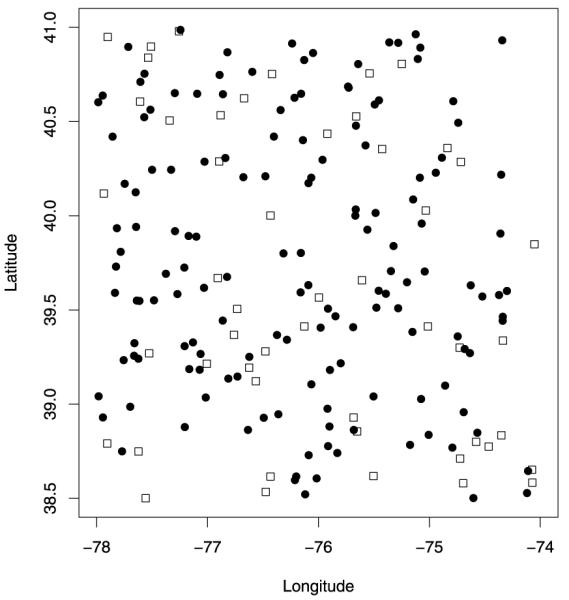
Validation (squares) and test sites (black dots) used to assess the predictive performance of Bayesian melding and the downscaler on the simulated data.
Figure 4.

(a) Simulated observed process at CMAQ grid cells, obtained by adding a white noise process, sampled from a N(0, 0.02) distribution, to the simulated true process. Predictive surface at CMAQ grid cells as obtained using: (b) Bayesian melding and (c) our downscaler. The legend for panels (a)–(c) is provided below panel (a). Color versions of panels (a)–(c) are available in the online appendix with supplemental material.
To generate values for the observed process under Bayesian melding, we first simulated the true unobserved Gaussian process at all the 200 sites, then we added to it an error term, sampled independently at each site from a N(0, 0.02) distribution. The underlying truth was generated by sampling from a 200-dimensional multivariate normal distribution with an exponential correlation structure with a decay parameter of 0.01. This means that the spatial correlation in the underlying truth drops below 0.05 at a distance greater or equal to log(0.05)/0.01 = 299.6 km, which is approximately two-thirds of the maximum width of the region.
Under Bayesian melding, simulation of the numerical model output involves computation of stochastic integrals. We approximate these integrals with averages using, for each grid cell, a systematic sample of four sites at which we have simulated values of the true process. We then computed the second-degree polynomial representing the spatially-varying additive bias of the numerical model output, and for each grid cell, we have derived the value of the numerical model output at the grid cell by simply averaging the bias-corrected truth at the four sites to which we had added an error term. We have used the following illustrative values in our simulation: we set the multiplicative bias to 0.9, we took the coefficients of the second-degree polynomial, representing the additive bias, to be equal to, respectively, 1.2, 0.9, −0.6, 0.03, −0.5, and 0.07, and we set the variance of the error measurement for the model output to 0.01.
Once the data was simulated, we estimated the parameters of Bayesian melding and of our downscaler via MCMC. Since, in Bayesian melding, the multiplicative bias of the numerical model output is assumed to be constant in space, in fitting our static downscaler, we set the local adjustment β1(s) to zero.
We compared the predictive performance of Bayesian melding and our downscaling model by looking at the mean squared error (MSE), mean absolute error (MAE), and variance of the predictions at the 50 validation sites. We have also computed the empirical coverage and average length of the 90% predictive intervals. The MSE and MAE were, respectively, 80.5 and 7.9 for Bayesian melding, and 34.3 and 4.6 for our downscaling method, indicating that, despite the fact that the data were simulated under Bayesian melding, our downscaler produces predictions that are less biased. The downscaler outperforms Bayesian melding also in terms of empirical coverage of the 90% predictive intervals. The coverage and average length of the predictive intervals were, respectively, 60.0% and 10.4 for Bayesian melding, and 82.0% and 15.7 for our downscaler. The shorter length of the predictive intervals for Bayesian melding is due to the fact that Bayesian melding has a smaller predictive variance than that of the downscaler: 10.4 versus 23.4, respectively. This is partly due to the fact that we used an empirical Bayes approach in estimating the parameters of the melding model.
In addition to generating predictions at validation sites, we also produced predictions at the numerical model grid cells centroids. Figure 4 shows the simulated values of the observation process at the model grid cells in panel (a), while it presents the predictive surface at the model grid cells for Bayesian melding and the downscaler in panels (b) and (c), respectively. The Bayesian melding predictive surface in Figure 4(b), probably as a result of following the numerical model, tends to predict values that are lower than the simulated values for the observation process in the southwestern corner. Additionally, it does not seem to capture the spatial pattern in the observation process. On the other hand, the predictive surface produced by our downscaler model, despite being much smoother than Figure 4(a), does a better job at capturing the spatial East–West gradient of the observation process.
We also constructed 90% predictive intervals at the model grid cells and we computed their respective lengths. As for the predictive intervals at observation sites, predictive intervals obtained under Bayesian melding are shorter than the intervals constructed using our downscaler model. The average length of the 90% predictive intervals at the numerical model grid cells was 10.4 for Bayesian melding versus 19.8 for our downscaler model. In summary, Bayesian melding, were we able to implement it over the spatial and temporal scales of interest, will be too optimistic. The downscaler will tend to be conservative, likely due to some overfitting effects. It is possible to reduce the width of the predictive intervals obtained under our downscaler model using an empirical Bayes approach within our framework as we take up in the Discussion section. However, further empirical investigation will be needed to assess how well this strategy works.
4.1.2. Ozone Data
To investigate the predictive performance of the static downscaler on ozone data, we consider three illustrative dates, randomly chosen: one in June, one in July, and one in August. For each day, we fit our downscaler using ozone observations coming from 69 monitoring sites and estimates of average ozone concentration over the associated grid cell provided by CMAQ. For comparison, we fit Bayesian melding using the 69 observations and CMAQ model output for the 651 grid cells covering the subset region displayed in Figure 1(b). For ordinary kriging, we estimate parameters of the exponential covariance function using only the 69 observations. The mean and standard deviation of the observed daily 8 hr maximum ozone concentration for the three days were, respectively, 69.94 and 14.28 ppb for June 21, 2001; 72.23 and 9.61 ppb for July 10, 2001; and 41.78 and 13.96 ppb for August 11, 2001.
After estimating the model parameters, we proceeded to predict ozone concentration at all of the 69 monitoring sites using the three different methods. As with the simulated data, we evaluate the quality of the predictions by computing the MSE and MAE of the predictions, and by looking at the empirical coverage and average length of the 90% predictive intervals. Table 1 reports these summary statistics for all three selected days. As the table shows, the downscaler produces predictions that are far better calibrated than the other methods. Moreover, the empirical coverage of our downscaler is always above the nominal value, thus indicating that our model is more conservative than Bayesian melding, whose empirical coverage is always below 90%. Alternatively, the predictive intervals constructed using the downscaler are wider than those obtained using Bayesian melding, which in turn are too narrow.
Table 1.
Mean square error (MSE), mean absolute error (MAE), empirical coverage, average length of 90% predictive intervals (PI) and predictive variance for ordinary kriging, Bayesian melding and the downscaler method for three days in the 2001 high-ozone season.
| Day | Method | MSE | MAE | Empirical coverage of 90% PI |
Average length of 90% PI |
Average predictive variance |
|---|---|---|---|---|---|---|
| 06/21/2001 | Ordinary kriging | 37 | 4.9 | 90% | 21 | 40 |
| Bayesian melding | 35 | 4.8 | 78% | 14 | 19 | |
| Downscaler | 10 | 2.5 | 99% | 19 | 35 | |
| 07/10/2001 | Ordinary kriging | 39 | 4.7 | 96% | 23 | 48 |
| Bayesian melding | 32 | 4.3 | 88% | 17 | 26 | |
| Downscaler | 16 | 2.9 | 97% | 21 | 43 | |
| 08/11/2001 | Ordinary kriging | 31 | 4.4 | 91% | 21 | 41 |
| Bayesian melding | 15 | 3.0 | 79% | 12 | 13 | |
| Downscaler | 6 | 1.9 | 97% | 17 | 29 |
Ordinary kriging performs as well as the downscaler model in terms of coverage and average length of the 90% predictive intervals, but its predictions are much more biased than the ones produced using our downscaling model. This might be expected since ordinary kriging does not exploit the additional information contained in the high resolution CMAQ output, relying only on the 69 ozone observations.
Our downscaler model allows us to construct maps of the spatial additive bias. Figure 5 shows, respectively, the posterior predictive mean of the spatial additive bias β0(s) and its corresponding standard deviation, both on the square root scale. As Figure 5 shows, the additive bias of the square root of the numerical model output varies locally, ranging from −2.02 to 0.95 ppb. Calibration on the original scale is clearly needed but more complicated to express. In particular, the figure shows that CMAQ has a negative bias in the central part of the region, it has an almost null bias on the southeastern part of the region, and it is positively biased in the southwestern corner. Also, the uncertainty associated with the estimate of the additive bias varies spatially, being smaller near where monitoring sites are located.
Figure 5.

(a) Posterior predictive mean and (b) standard deviation for the spatially-varying additive bias, β0(s) of the CMAQ output for August 11, 2001. Color versions of panels (a)–(b) are available in the online appendix with supplemental material.
We have also predicted the daily 8 hr maximum ozone concentration at the 651 CMAQ grid cells under the three methods. Figure 6(a) shows the observed ozone concentration at the 69 monitoring sites on August 11, 2001. Figure 6(b) displays the CMAQ predicted average ozone concentration over the region for that day, while Figures 6(c) through (e) present the predictive surfaces obtained using ordinary kriging, Bayesian melding, and our downscaler, respectively. As Figure 6(b) shows, the CMAQ model output is biased, estimating values of ozone concentration that are much more elevated than what was actually observed. Both Bayesian melding and the downscaler revise the CMAQ model output, and, due to the information contained in the observations, predict values of ozone that are lower than CMAQ. On the other hand, ordinary kriging uses only the information contained in the observations to yield a predictive surface that is arguably too smooth for the entire region. Bayesian melding yields a predictive surface that retains the high values estimated by CMAQ in the parts of the region that are unmonitored, while it pushes down CMAQ wherever there are monitoring sites. However, the gradient in the Bayesian melding predictive surface of ozone concentration follows quite closely the gradient of the CMAQ surface. On the other hand, the predictive surface of ozone concentration obtained using the downscaler model lies between the ordinary kriging and the Bayesian melding predictive surfaces. It shows a central region with lower ozone values, as the observations seem to indicate, but its gradient is a combination of the overly smooth gradient of the ordinary kriging predictive surface and the gradient of the CMAQ surface.
Figure 6.


(a) Observed ozone on August 11, 2001. Predicted ozone surface for August 11, 2001 as provided by: (b) CMAQ; (c) ordinary kriging; (d) Bayesian melding; and (e) the downscaler method. The legend for panels (a)–(e) is provided beside panel (a). Color versions of panels (a)–(e) are available in the online appendix with supplemental material.
4.2. Spatio-Temporal Model
We now describe the verification results for the spatio-temporal version of our downscaler. As mentioned in Section 3.1, there are different ways in which the static downscaler can be extended to include the temporal dimension. Table 2 reviews the eight models that we have considered. In particular, for Models 1 through 4, we have evaluated whether the multiplicative bias of CMAQ model output should be assumed as varying in space or constant over space, as postulated in Bayesian melding. Thus, for each model, we have developed two versions, one where the local adjustment β1(s) to the overall bias term β1 is set equal to 0, implying a spatially-constant multiplicative bias, and one where β1(s) is nonnull. Each of the eight models was fit using both ozone monitoring data coming from 436 of the total 803 NAMS/SLAMS monitoring sites located in the eastern U.S., and the corresponding CMAQ model output at the associated 12 km grid cells. The remaining 367 monitoring sites, each having more than one missing value during the period May 1–October 15, 2001, were held out and used for validation.
Table 2.
Various spatio-temporal versions of the static downscaler model.
| Model | β1t (s) |
β
0t β 1t |
β0t (s) β1t (s) |
|---|---|---|---|
| Model 1 | ≠ 0 | Independent across time | Constant in time |
| Model 1a | = 0 | Independent across time | Constant in time |
| Model 2 | ≠ 0 | Dynamic | Constant in time |
| Model 2a | = 0 | Dynamic | Constant in time |
| Model 3 | ≠ 0 | Independent across time | Independent across time |
| Model 3a | = 0 | Independent across time | Independent across time |
| Model 4 | ≠ 0 | Dynamic | Dynamic |
| Model 4a | = 0 | Dynamic | Dynamic |
The eight different spatio-temporal versions of our downscaler were compared on the basis of the same summary statistics as above: the MSE and MAE of the predictions, the empirical coverage and average length of the 90% predictive intervals, and the predictive variance. Among all models, the one that gave the best verification results was Model 3a, that is, the model with spatially-constant multiplicative bias, where both the overall bias terms, β0t and β1t , and the local adjustment to β0t , β0t (s,t), were modeled as independent across time, as shown in Equations (3.5) and (3.8).
We subsequently compared the predictions obtained using Model 3a with the predictions yielded by ordinary kriging. Details on how we performed ordinary kriging in the spatio-temporal setting were provided in Section 3.4. Table 3 presents the MSE, MAE, empirical coverage, average length of the 90% predictive intervals, and average predictive variance for the two methods. As the table shows, the spatio-temporal version of the downscaler provided by Model 3a gives predictions that are better calibrated than those obtained with ordinary kriging. Additionally, the predictive intervals have better empirical coverage.
Table 3.
Mean square error (MSE), mean absolute error (MAE), empirical coverage and average length of 90% predictive intervals for ordinary kriging and for the selected spatio-temporal version of the downscaler.
| Method | MSE | MAE | Empirical coverage of 90% PI |
Average length of 90% PI |
|---|---|---|---|---|
| Ordinary kriging | 61 | 5.7 | 72% | 18 |
| Spatio-temporal downscaler | 50 | 5.2 | 88% | 21 |
Our spatio-temporal downscaler enables usual summaries: (i) constructing maps of the spatial bias in the numerical model output aggregated at any desired temporal resolution, (ii) deriving improved maps of ozone concentration at any desired spatial resolution and aggregated to any desired temporal summary, (iii) constructing maps of the corresponding uncertainty associated with the predictions. In addition, we consider another by-product of our model which is strictly related to air quality standards. The current National Ambient Air Quality Standard (NAAQS) for ozone, proposed by the EPA, is that the 3-year rolling average of the annual fourth highest daily 8 hr maximum average ozone concentration be less than 80 ppb (for reference, see http://www.epa.gov/air/criteria.html). Unfortunately our dataset does not span three years. However, for illustration, we can produce a map of the predicted surface of the fourth highest daily 8 hr maximum ozone concentration during the period May 1–October 15, 2001. Figure 7 presents a map of the posterior predictive mean of the fourth highest ozone concentration during the 168 day long high-ozone season in panel (a), while it shows a map of the posterior predictive standard deviation in panel (b). Evidently, there is considerable spatial variability in this measure with greater uncertainty where monitoring is more sparse, but overall the predictive variances are small relative to the predictions.
Figure 7.

(a) Posterior predictive mean and (b) posterior predictive standard deviation of the 4th highest ozone concentration during the period May 1–October 15, 2001. Color versions of panels (a)–(b) are available in the online appendix with supplemental material.
Additionally, Figure 8 displays a map of the probability that the fourth highest ozone concentration during the period May 1–October 15, 2001 exceeds two different thresholds: the first one is the current ozone standard of 80 ppb, the second one is the stricter threshold of 75 ppb. For display purposes, both of these maps have been obtained at the CMAQ 12 km grid cell resolution, but it is within the capabilities of our model to produce local maps at a finer spatial resolution. Note that Figures 8(a) and (b) cannot be interpreted as probabilities that a site is in compliance with the NAAQS ozone standard, since that is given in terms of 3-year rolling averages. However, they give a clear indication of the status of air quality over the eastern U.S. If the NAAQS ozone standard were decreased to 75 ppb, most of the eastern U.S. would have a high probability of not being in compliance, as Figure 8(a) shows. With the current standard of 80 ppb, limiting ourselves only to the high-ozone season for one year, we can conclude that the probability that the threshold of 80 ppb is exceeded is fairly low almost everywhere in the eastern U.S.
Figure 8.

Posterior predictive probability that the 4th highest ozone concentration during the period May 1–October 15, 2001 is above (a) 75 ppb and (b) above 80 ppb. The dots show the observed occurrence that the 4th highest ozone concentration is above 75 ppb and 80 ppb, respectively. Color versions of panels (a)–(b) are available in the online appendix with supplemental material.
5. DISCUSSION
In this article, we presented a model to address the “change of support” problem when the interest is in inferring a spatial process at the point level given areal data represented by numerical model output. Our downscaling approach is fully model-based but it is not a fusion model. Instead, it takes the numerical model output as data and models the relationship between observations and numerical model output via a linear regression with spatially varying coefficients assumed to arise from correlated spatial Gaussian processes. Our model specification is simple, flexible, and it allows a very natural extension to the spatio-temporal setting. From a computational point of view, our model benefits from a specification that does not involve stochastic integration as Bayesian melding does. That is, in fitting the melding model, all the numerical model grid cells are used. In fitting our downscaler only those grid cells of the numerical model, where observations have been collected, are used.
There are several interesting and useful applications to both our static and spatio-temporal downscaler. Firstly, it allows us to identify regions in the spatial domain where the numerical model is more biased. Such information can be extremely valuable to those who develop numerical models. Secondly, it allows us to construct maps of improved predictions at any desired spatial resolution and at any desired temporal summary. Such maps can then be used for environmental regulatory purposes as well as for decision making strategies. Finally, in the context of air quality, our downscaler permits the computation of probabilities of exceeding thresholds.
There are several ways in which our model could be extended. First, we have developed the downscaler for a variable that follows, either in its original scale or via some appropriate transformation, a Gaussian distribution. A natural extension could develop a downscaling model for non-Gaussian first stage distributions. This could be achieved by introducing a latent Gaussian process and then using the downscaler on the latent variable as, for example, in the framework of generalized linear models in Diggle, Moyeed, and Tawn (1998). In the dynamic models, if appropriate, we might consider extending our specification to allow for time-varying spatial decay parameters. Finally, it is possible to introduce empirical Bayes elements within our modeling framework. For instance, by using data from previous seasons, one could perform, at each site, a linear regression of the observations on the numerical model output at the grid cell containing the site under consideration. This will yield, at each site, estimates of the additive and multiplicative bias which can be fixed within the MCMC. Spatial decay parameters in the coregionalization could also be fixed, perhaps developed through the above regressions. In any event, the effects of replacing estimation with integration would need to be investigated empirically before their use could be recommended.
Finally, as pollutants are likely to be correlated, another interesting extension of this work would be to develop a multivariate version of the downscaler. A by-product of such a model would be the possibility of deriving improved predictions of several pollutants jointly or separating diurnal from nocturnal ozone levels. Such analysis could advance our knowledge regarding the relationships and interactions between air pollutants and human health.
Supplementary Material
ACKNOWLEDGEMENT
The authors thank Serge Guillas and Sujit Sahu for useful conversations. This research was facilitated through grant RD-83329301-0 from the Environmental Protection Agency and grant P20-RR020782-03 from the National Institutes of Health.
Footnotes
SUPPLEMENTAL MATERIALS Illustrations: Supplemental materials contain the color versions of Figures 4–8, the trace plots for the static version of the downscaler with β1(s) = 0 for August 11, 2001 and the trace plots for some of the parameters of the spatio-temporal version of the downscaler with β0t ,β1t ,β0(s,t),β1(s,t) modeled as independent replicates. Also the U.S. Environmental Protection Agency’s Office of Research and Development partially collaborated in the research described here. Although it has been reviewed by the EPA and approved for publication, it does not necessarily reflect the Agency’s policies or views. supplement. (13253_2009_4_MOESM1_ESM.pdf, 13253_2009_4_MOESM2_ESM.pdf, 13253_2009_4_MOESM3_ESM.pdf, 13253_2009_4_MOESM4_ESM.pdf, 13253_2009_4_MOESM5_ESM.pdf, 13253_2009_4_MOESM6_ESM.pdf, 13253_2009_4_MOESM7_ESM.pdf, 13253_2009_4_MOESM8_ESM.pdf)
Contributor Information
Veronica J. Berrocal, Department of Statistical Science, Duke University, Durham, NC 27708, USA.
Alan E. Gelfand, Department of Statistical Science, Duke University, Durham, NC 27708, USA (alan@stat.duke.edu)..
David M. Holland, U.S. Environmental Protection Agency, National Exposure Research Laboratory, Research Triangle Park, NC 27711, USA (holland.david@epa.gov)..
REFERENCES
- Banerjee S, Carlin BP, Gelfand AE. Hierarchical Modeling and Analysis for Spatial Data. Chapman & Hall/CRC; Boca Raton, FL: 2004. [Google Scholar]
- Carroll SS, Day G, Cressie N, Carroll TR. Spatial Modeling of Snow Water Equivalent Using Airborne and Ground-Based Snow Data. Environmetrics. 1995;6:127–139. [Google Scholar]
- Carter C, Kohn R. On Gibbs Sampling for State Space Models. Biometrika. 1994;81:541–553. [Google Scholar]
- Chilès J-P, Delfiner P. Geostatistics: Modeling Spatial Uncertainty. Wiley; New York: 1999. [Google Scholar]
- Cowles MK, Zimmerman DL. A Bayesian Space-Time Analysis of Acid Deposition Data Combined From Two Monitoring Networks. Journal of Geophysical Research. 2003;108(D24):9006. doi: 10.1029/2003JD004001. [Google Scholar]
- Cowles MK, Zimmerman DL, Christ A, McGinnis DL. Combining Snow Water Equivalent Data From Multiple Sources to Estimate Spatio-Temporal Trends and Compare Measurement Systems. Journal of Agricultural, Biological and Environmental Statistics. 2002;7:536–557. [Google Scholar]
- Cressie NAC. Statistics for Spatial Data. Wiley; New York: 1993. [Google Scholar]
- Denison DGT, Mallick BK, Smith AGM. Automatic Bayesian Curve Fitting. Journal of the Royal Statistical Society, Ser. B. 1998;60:333–350. [Google Scholar]
- Diggle PJ, Moyeed RA, Tawn JA. Model-Based Geostatistics (with discussion) Applied Statistics. 1998;47:299–350. [Google Scholar]
- Dominici F, Daniels M, Zeger SL, Samet JM. Air Pollution and Mortality: Estimating Regional and National Dose-Response Relationships. Journal of the American Statistical Association. 2002;97:100–111. [Google Scholar]
- Foley KM, Fuentes M. A Statistical Framework to Combine Multivariate Spatial Data and Physical Models for Hurricane Wind Prediction. Journal of Agricultural, Biological and Environmental Statistics. 2008;13:37–59. [Google Scholar]
- Fuentes M, Raftery AE. Model Evaluation and Spatial Interpolation by Bayesian Combination of Observations With Outputs From Numerical Models. Biometrics. 2005;61:36–45. doi: 10.1111/j.0006-341X.2005.030821.x. [DOI] [PubMed] [Google Scholar]
- Fuentes M, Song H-R, Ghosh SK, Holland DM, Davis JM. Spatial Association Between Speciated Fine Particles and Mortality. Biometrics. 2006;62:855–863. doi: 10.1111/j.1541-0420.2006.00526.x. [DOI] [PubMed] [Google Scholar]
- Gelfand AE, Banerjee S, Gamerman D. Spatial Process Modelling for Univariate and Multivariate Dynamic Spatial Data. Environmetrics. 2005;16:465–479. [Google Scholar]
- Gelfand AE, Kim H-J, Sirmans CF, Banerjee S. Spatial Modeling With Spatially Varying Coefficient Processes. Journal of the American Statistical Association. 2003;98:387–396. doi: 10.1198/016214503000170. [DOI] [PMC free article] [PubMed] [Google Scholar]
- Gelfand AE, Schmidt AM, Banerjee S, Sirmans CF. Nonstationary Multivariate Process Modeling Through Spatially Varying Coregionalization. TEST. 2004;13:263–312. [Google Scholar]
- Gotway CA, Young LJ. Combining Incompatible Spatial Data. Journal of the American Statistical Association. 2002;97:632–648. [Google Scholar]
- — — — A Geostatistical Approach to Linking Geographically Aggregated Data From Different Sources. Journal of Computational and Graphical Statistics. 2007;16:115–135. [Google Scholar]
- Green PJ. Reversible Jump Markov Chain Monte Carlo Computation and Bayesian Model Determination. Biometrika. 1995;82:711–732. [Google Scholar]
- McMillan N, Holland DM, Morara M, Feng J. Combining Numerical Model Output and Particulate Data Using Bayesian Space-Time Modeling. Environmetrics. 2009 to appear. [Google Scholar]
- Poole D, Raftery AE. Inference for Deterministic Simulation Models: The Bayesian Melding Approach. Journal of the American Statistical Association. 2000;95:1244–1255. [Google Scholar]
- Sahu SK, Gelfand AE, Holland DM. Spatio-Temporal Modeling of Fine Particulate Matter. Journal of Agricultural, Biological and Environmental Statistics. 2006;11:61–86. [Google Scholar]
- Schmidt AM, Gelfand AE. A Bayesian Coregionalization Approach for Multivariate Pollutant Data. Journal of the Geophysical Research. 2003;108(D24):8783. doi: 10.1029/2002JD002905. [Google Scholar]
- Smith BJ, Cowles MK. Correlating Point-Referenced Radon and Areal Uranium Data Arising From a Common Spatial Process. Applied Statistics. 2007;56:313–326. [Google Scholar]
- Tolbert P, Mulholland J, MacIntosh D, Xu F, Daniels D, Devine O, Carlin BP, Klein M, Dorley J, Butler A, Nordenberg D, Frumkin H, Ryan PB, White M. Air Pollution and Pediatric Emergency Room Visits for Asthma in Atlanta. American Journal of Epidemiology. 2000;151:798–810. doi: 10.1093/oxfordjournals.aje.a010280. [DOI] [PubMed] [Google Scholar]
- Wackernagel H. Multivariate Geostatistics. 2nd ed Springer; Berlin: 1998. [Google Scholar]
- West M, Harrison J. Bayesian Forecasting and Dynamic Models. 2nd ed Springer-Verlag; New York: 1999. [Google Scholar]
- Wikle CK, Berliner LM. Combining Information Across Spatial Scales. Technometrics. 2005;47:80–91. [Google Scholar]
- Zhang H. Inconsistent Estimation and Asymptotically Equal Interpolations in Model-Based Geostatistics. Journal of the American Statistical Association. 2004;99:250–261. [Google Scholar]
- Zhu L, Carlin BP, Gelfand AE. Hierarchical Regression With Misaligned Spatial Data: Relating Ambient Ozone and Pediatric Asthma ER Visits in Atlanta. Environmetrics. 2003;14:537–557. [Google Scholar]
Associated Data
This section collects any data citations, data availability statements, or supplementary materials included in this article.