Bimodal gene expression in noncooperative regulatory systems

Abstract

Bimodality of gene expression, as a mechanism contributing to phenotypic diversity, enhances the survival of cells in a fluctuating environment. To date, the bimodal response of a gene regulatory system has been attributed to the cooperativity of transcription factor binding or to feedback loops. It has remained unclear whether noncooperative binding of transcription factors can give rise to bimodality in an open-loop system. We study a theoretical model of gene expression in a two-step cascade (a deterministically monostable system) in which the regulatory gene produces transcription factors that have a nonlinear effect on the activity of the target gene. We show that a unimodal distribution of transcription factors over the cell population can generate a bimodal steady-state output without cooperative transcription factor binding. We introduce a simple method of geometric construction that allows one to predict the onset of bimodality. The construction only involves the parameters of bursting of the regulatory gene and the dose–response curve of the target gene. Using this method, we show that the gene expression may switch between unimodal and bimodal as the concentration of inducers or corepressors is varied. These findings may explain the experimentally observed bimodal response of cascades consisting of a fluorescent protein reporter controlled by the tetracycline repressor. The geometric construction provides a useful tool for designing experiments and for interpretation of their results. Our findings may have important implications for understanding the strategies adopted by cell populations to survive in changing environments.

This paper proves theoretically that bimodality of gene expression can be generated in a minimal gene regulatory system by a unimodal distribution of transcription factor (TF) combined with a nonlinear transcription rate, without cooperativity, large number of steps in gene cascade, feedback loops, or bimodal input signal. We present a method of prediction of the bimodality without using the master equation, only based on a simple geometric construction.

Bimodal gene expression (the distribution of gene products that has two maxima) is a cause of phenotypic diversity in genetically identical cell populations, and it is critical for population survival in a fluctuating environment (1–4). Several mechanisms underlying the bimodality have been identified to date:

1. Deterministic bistability (two deterministic stable steady states under the same external conditions) is inherent to the system even when intrinsic and extrinsic noises can be neglected. To exhibit deterministic bistability, the system must consist of a single positive feedback loop with cooperative ligand binding (5, 6) [bacteriophage λ (7), reverse tetracycline transactivator switch in Saccharomyces cerevisiae (8), lac operon in Escherichia coli (9), MAPK cascade in Xenopus oocytes (10)], multiple feedback loops with cooperativity (6, 11, 12) [Ptrc-2/P1 toggle switch (13)], or multiple feedback loops without cooperativity (14).

2. When the system is described as a continuous dynamical system with multiplicative noise, the noise can induce a bimodal response, which would not occur in a deterministic case. (i) Shift of the bistability range due to noise. In a system that can be bistable in a certain range of parameters, but its current parameters place it in a monostable regime, the fluctuations can shift or stretch the range of parameters required for bistability to make the system effectively bistable (15–17) [Gal regulatory network (18)]. (ii) Emergence of bistability due to noise. Theoretical studies predict that multiplicative noise can introduce bifurcations in systems that are monostable for all parameter ranges (17, 19–22).

3. Bimodality due to transcriptional pulsing (BTP) is caused by random switching of the operator between ON and OFF states. Although plenty of experimental evidence exists for transcriptional pulsing, its origins are still largely unknown (23, 24). Theoretical works predict BTP in closed-loop systems (25) as well as in open-loop (monostable) systems (26–31). In this paper, we refer only to one of the hypothesized sources of transcriptional pulsing; namely, the discrete random binding/unbinding of TFs. In that case, BTP arises when the average time between the binding and unbinding events is greater than the time scales of other processes in the system. The rare events of TF binding change the position of the deterministic steady state from maximum production to total repression, allowing the system enough time to settle down in these states (26, 31). When the amount of TF is constant across the cell population, the product distribution converges to unimodal as TF binding/unbinding becomes too frequent for the target gene to respond (30).

Recent studies on the bimodality of gene expression have focused on the search for this effect in the systems that are different from those listed above: deterministically monostable closed-loop systems with noncooperative TF binding (32) and open-loop systems with cooperative TF binding (33–37). However, it has remained unclear how the cooperativity is connected to bimodality in those systems and whether the noncooperative binding of TFs can give rise to bimodality in open-loop cascades.

The goal of our work is to answer these questions. We consider the model of gene expression in a two-step cascade (a minimal open-loop system) in which the regulatory gene produces TFs that have a nonlinear effect on the activity of the target gene. The transcription rate of the target gene can be then described as a nonlinear function of the TF concentration in a given cell. We will refer to this function as the transfer function (38). We assume that TF molecules are unimodally distributed across the cell population because of translational bursting of the regulatory gene and cell division (39, 40). The transfer function acts as a nonlinear noise filter, transforming the unimodal TF distribution (input noise) into the bimodal distribution of transcription rates in the cell population (output noise).

In the qualitative considerations of Niepel et al. (41) and Kaern et al. (30), a sigmoidal transfer function (i.e., cooperative TF binding) was assumed as the underlying cause of the noise filter induced bimodality (NFIB). Examples of NFIB have been obtained by numerical calculation in two theoretical works (34, 36). In ref. 34 this effect was observed only in highly cooperative cascades of three or more genes, whereas in ref. 36 it was attributed to high cooperativity in a two-gene cascade. However, these works did not provide a rigorous analysis of the mechanism of NFIB nor conditions for the bimodality. In the experimental studies of open-loop tetracycline repressor (TetR)-based cascades with cooperative TF binding (33, 35, 37) and closed-loop Tet-Off cascades with autoregulation of the noncooperative tTA activator (32), bimodal gene expression was observed as a result of noise in TF production.

There are no theoretical studies on the conditions for NFIB to occur and, in particular, on the possibility of its occurrence in noncooperative systems. In this paper, we prove by analytical calculation of the conditions for NFIB that bimodality can occur in the minimal gene cascade with noncooperative TF binding.

Model

We consider the model of gene expression in a two-step cascade (Fig. 1). The regulatory gene produces TFs that control the production of a target protein from the target gene. The distribution of TFs across the cell population is nonuniform because of stochastic effects in gene expression (30, 42). We assume that these effects are dominated by translational bursting of the regulatory gene and cell division (39, 40), which are much slower than transcription and translation from the target gene, so that the amount of TF in each cell in the population can be considered constant within the time scales of synthesis and degradation of the target gene products. For a large number R of TFs, their stationary distribution tends to the continuous gamma distribution (28, 39, 40) (Fig. S1):

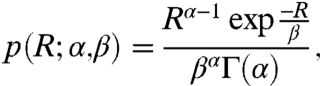[1]

where α is the mean number of TF production bursts per cell cycle, and β is the average size of the TF production bursts. (All distributions that we consider in this paper are stationary distributions.)

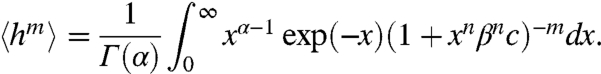
Fig. 1.

Nonlinear transcription rate transforms a unimodal distribution of TFs into a bimodal distribution of target proteins. Transcription is regulated by TFs (here, repressors) R, which bind to n binding sites within operator region, with or without cooperativity. Transcription rate is proportional to a nonlinear function of TF number (transfer function) h(R). The figure shows the most simple case: noncooperative binding, with h(R) given by Eq. 2 with n = 1, TF binding rate k_on, and unbinding rate k_off. mRNA M degrades with rate k_dm. The target protein P is produced with rate k_p and degrades with rate k_dp. The transfer function h(R) acts as a nonlinear noise filter that transforms the unimodal input [TF distribution p(R) generated by the regulatory gene] into a bimodal output [distribution q(h) of the rates of transcription from the target gene]. Consequently, the distributions of mRNA p_mrna(M) and the target protein p_prot(P) are bimodal.

We assume that TF binding and unbinding are the fastest reactions in the system and that TF production and degradation are the slowest reactions in the system (15, 43). On the contrary to BTP, the average time between the events of TF binding and unbinding is then shorter than the time of relaxation of the target gene to its steady state. The rate of transcription from the target gene is then proportional to a nonlinear function h(R) (the transfer function). From now on, we will analyze as a working example the system where TFs are repressors. In the case of activation, all the calculations presented below are valid with the substitution h^′(R) = 1 - h(R). For a noncooperative binding of n repressors,

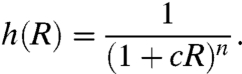[2]

For a strongly cooperative binding of n repressors (i.e., when the maximum occupation of binding sites dominates),

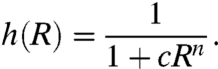[3]

n≥1 is the number of repressor binding sites and c is the ratio of binding to unbinding rates for each repressor (see SI Model for detailed analysis).

Results

Unimodal TF Distribution Can Generate a Bimodal Distribution of Transcription Rates.

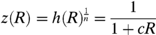
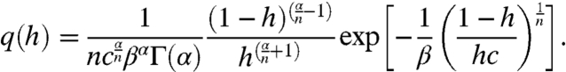
The transfer function h(R) transforms the distribution of repressors p(R) into the distribution q(h) of transcription rates (SI Results). For noncooperative binding of n repressors,

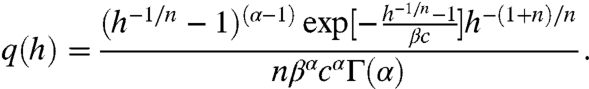[4]

The extrema of q(h) are defined by the intersection points of the rescaled transfer function given by Eq. 2:

[5]

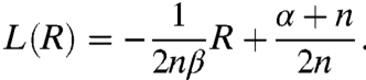
and the straight line (see SI Results for derivation):

[6]

Fig. 2 A and B shows that two cases should be considered, depending on the frequency of repressor production bursts α. For α < 1, a maximum at h = 1 exists, independent of the intersections, and another maximum emerges when L(R) has a sufficiently small slope (large β) to intersect with z(R). For α > 1, there is always one intersection, which defines the only maximum, and thus bimodality in the transcription-rate distribution is impossible in this regime. For the cooperative binding of n repressors,

[7]

The extrema of q(h) are defined by the intersection points of the transfer function given by Eq. 3 and the straight line

[8]

Fig. 2 C and D also shows two cases. For α < n, a maximum at h = 1 exists, independent of the intersections, and another maximum emerges when L(R) intersects with h(R). For α > n, all extrema are defined by the intersections, and two maxima can emerge only in a narrow range of β, when L(R) intersects h(R) three times. The above findings have been summarized in Table S1. For the noncooperative case, the moments of q(h) are given by

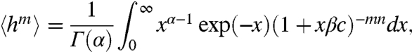[9]

and for the cooperative case,

[10]

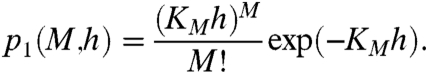
The analytical solutions of Eqs. 9 and 10, although lengthy, are easily obtained using a symbolic algebra software (see Eqs. S39–S41). Further on, we will focus on the case of noncooperative TF binding, and the analogous analysis of the cooperative case is presented in SI Results. The variance of q(h) can be considered a measure of its bimodality. From the geometric construction it follows that the maximal variance 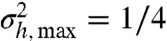is obtained for a maximally bimodal q(h) = [δ(h) + δ(h - 1)]/2; i.e., the sum of two Dirac delta functions. In the bimodal regime of α and β, the stronger the bimodality is, the higher (Fig. 3 A and B).

Fig. 2.

Geometric construction of the conditions for bimodal distribution of transcription rates q(h) in systems with noncooperative (A and B) and cooperative (C and D) binding of n repressors. The extrema of q(h) are the points of intersection of the rescaled transfer function z(R) (Eq. 5) and the straight line L(R) (Eq. 6) (noncooperative case), or the transfer function h(R) (Eq. 3) and the straight line L(R) (Eq. 8) (cooperative case). A and B show the simplest case of noncooperativity, with n = 1 and z(R) = h(R). The height at which L(R) intersects the vertical axis depends on the number α of repressor production bursts per cell cycle. The slope of L(R) depends on the number β of repressor molecules produced per burst. The dashed and gray solid lines show examples without intersections, which generate monomodal distributions. (A) Noncooperative binding. For α < 1, a maximum at h = 1 exists, independent of the intersections, and another maximum emerges at the lower point of intersection. (B) Noncooperative binding. For α > 1, there is always one intersection, defining the only maximum, and thus bimodality is impossible. (C) Cooperative binding. For α < n, a maximum at h = 1 exists, independent of the intersections, and another maximum emerges at the lower point of intersection. (D) Cooperative binding. For α > n, all extrema are defined by the intersections. Two maxima can emerge only when L(R) intersects h(R) three times. Parameters used for A: n = 1, c = 0.1, α = 0.5, β₁ = 50 (solid line), and β₂ = 15 (dashed line). Parameters used for B: n = 1, c = 0.1, β = 15, and α = 1.2. Parameters used for C: n = 2, c = 0.005, α = 0.9, β₁ = 20 (solid line), and β₂ = 10 (dashed line). Parameters used for D: n = 3, c = 0.0025, α = 4, β₁ = 2 (black solid line), β₂ = 1.6 (dashed line), and β₃ = 2.7 (gray solid line).

Fig. 3.

The variance of the transcription-rate distribution q(h) as a measure of bimodality of q(h) as well as mRNA and protein distributions. (A) The variance of q(h) depending on α and βc, noncooperative case with n = 1. White line, boundaries of the bimodal region. Above the white line, q(h) is bimodal. (B) The bimodality of q(h) increases as the of q(h) increases. q(h) is shown for α and βc marked in A by the points a, b, and c (α_a = 0.101, α_b = 0.25, α_c = 0.7, β = 20). (C and D) Protein distribution recovers the bimodality lost because of intrinsic noise at the mRNA level. (C) The distribution p₁(M,h = 1) has the variance , the distribution p₂(P,h = 1) has the variance , and . (D) causes the loss of bimodality of the mRNA distribution p_mrna(M), whereas at the protein distribution p_prot(P) is bimodal. k_m = 1, k_dm = 0.1, k_p = 0.5, k_dp = 0.01, k_on = 1, k_off = 10, k_mr = 5 × 10^-5, k_dmr = 0.01, k_r = 0.5, k_dr = 10^-4, and the other parameters are the same as in Fig. 2A with β₁.

Transcriptional and Translational Noises Decrease the Bimodality of Target mRNA and Protein Distributions.

Transcriptional and translational noises are the intrinsic noises due to a small number of molecules of mRNA or protein, respectively. In the presence of transcriptional noise, the stationary distribution of mRNA for a constant number of repressors is given by the Poisson distribution, with mean and variance K_Mh = k_mh/k_dm:

[11]

When both transcriptional and translational noises are present and k_dp ≪ k_dm, the target protein distribution for a constant number of repressors is approximated by the negative binomial distribution.

[12]

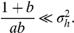
with ah = (k_m/k_dp)h being the number of protein production bursts per cell cycle, and b = k_p/k_dm being the number of protein molecules per burst (28). The mean is equal to abh and the variance is equal to abh(1 + b). For large P, Eq. 12 tends to the gamma distribution p(P; ah,b). To take into account the distribution p(R) of repressor molecules across the cell population, we convolve the distribution of transcription rates q(h) with the distributions of mRNA p₁(h,M) or proteins p₂(h,P). If q(h) is bimodal, then the resulting distribution of mRNA

[13]

and the distribution of proteins

[14]

may also be bimodal (Fig. 3D and Fig. S2). We integrated the theoretical distributions (Eqs. 13 and 14) numerically using the Maple software (Maplesoft). We compared them with the results of stochastic simulations, performed using the Gibson–Bruck version (44) of the Gillespie algorithm (45). The calculation of the Kullback–Leibler divergence between the theoretical and simulated distributions shows that the results are in an excellent agreement within the range of validity of the model (Figs. S2–S5). The bimodality of p_mrna and p_prot decreases and, finally, disappears as the intrinsic noises increase (Fig. S2).

Protein Distribution Can Recover the Bimodality Lost due to Intrinsic Noise at the mRNA Level.

Below, we derive an approximate method of estimating whether the bimodality persists in spite of the intrinsic fluctuations. The integrals of Eqs. 13 and 14 denote summation of the unimodal distributions p₁ (or p₂) with the weight q(h). If p₁ and p₂ were infinitely narrow, then p_mrna(M/K_M) and p_prot(P/(ab)) would exactly map q(h) (Eq. S43). The wider p₁ (or p₂) is, the more smeared out p_mrna (or p_prot) becomes compared to q(h). Within the integration range, p₁(M,h = 1) and p₂(P,h = 1) are the widest, and therefore they have the greatest possible contribution to smearing out the bimodality. When the variance of p₁(M/K_M,h = 1) [or p₂(P/(ab),h = 1)] is much smaller than the variance of q(h), then p_mrna (or p_prot) is bimodal (Fig. 3 A and B). For the mRNA distribution, the condition for bimodality can be written as

[15]

and for the protein distribution,

[16]

From 15 and 16, it follows that for small k_m/k_dm the mRNA distribution p_mrna loses the bimodality, but the protein distribution p_prot can recover the bimodality if k_p/k_dp is large (Fig. 3 C and D).

Intrinsic Noise due to TF Binding/Unbinding Increases the Bimodality of Target mRNA and Protein Distributions.

The formulas of Eqs. 13 and 14 for the mRNA and protein distributions neglect the intrinsic noise caused by the discrete nature of TF binding/unbinding, and thus they are valid when the kinetics of that process is faster than other reactions in the system. Using the simulations, we tested the behavior of the system beyond that range (SI Results). As the mean time between the consecutive events of TF binding and unbinding increases, the bimodality of the mRNA distribution abruptly increases when the slowest rate of the transcription process exceeds k_off, the slowest rate connected with TF binding/unbinding. Similarly, the bimodality of the protein distribution increases abruptly when k_off is smaller than the slowest rate of both transcription and translation stages. On those time scales a transition occurs between two types of bimodality that originate from two different phenomena: The NFIB (caused by fast TF binding/unbinding combined with a nonlinear dependence of protein transcription on TF abundance) makes a transition to BTP (caused by discrete, slow, TF binding/unbinding). The left peak of the distribution moves to zero because the mRNA or protein have enough time to totally degrade while the TF is bound to the operator. The right peak moves to the right, to the values corresponding to the maximum production of mRNA or protein in the total absence of TF. Because most protein lifetimes, in both eukaryotes (46, 47) and prokaryotes (48), are longer than mRNA lifetimes, an overlap is possible, where the mRNA distribution exhibits BTP but the protein distribution is still in the NFIB regime (Fig. S3 A–C). In this case, proteins respond to time-averaged fluctuations of mRNA level (28), but on the time scale of mRNA lifetime the operator state is no longer time-averaged (25). In the case of NFIB, each cell in the population remains at its own expression level because the TF binding/unbinding is much faster than the response of the target gene (Fig. S6A), whereas for BTP, individual cells switch their expression levels in time because the TF binding/unbinding is sufficiently slow for the target gene to respond (Fig. S6B).

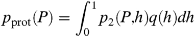
Bimodality of Target Protein Distribution Decreases as the Ratio of TF/Protein Lifetimes Decreases.

The model assumes TF production and degradation much slower than other processes in the system, so that each cell has a constant number R of TFs within the time scales of transcription and translation (Fig. S7). We tested the behavior of the system beyond that range (Fig. 4 and Figs. S3–S5). When the ratio of TF/protein lifetimes decreases, the protein distribution loses the bimodality (Fig. 4A). Fig. 4B shows the protein noise 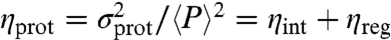depending on the ratio of TF/protein lifetimes. η_int = (1 + b)/(ab〈h〉) is the contribution from intrinsic noises, and η_reg is the regulatory noise (48, 49). When the TF lifetime is shorter than the protein lifetime, η_reg tends to zero. When the TF lifetime is longer than the protein lifetime, η_reg tends to the maximum regulatory noise . Fig. S8 shows that the nonmonotonic behavior of η_h for varying α and β is not connected with bimodality, on the contrary to the variance (Fig. 3). When the TF lifetime is comparable to the protein lifetime, the bimodality is no longer present, whereas the regulatory noise η_reg is still present (Fig. 4). This finding may explain the results of Taniguchi et al. (48), who did not detect evident bimodal distributions of proteins in E. coli, in spite of the fact that their study covered about one-fourth of the genome. They found, however, some regulatory noise contributions. We argue that the absence of bimodality could be the effect of long life of the studied YFP–protein fusions, which are more stable than native proteins (48), and therefore their lifetimes can be comparable or longer than the lifetimes of TFs responsible for the regulation. The same effect could also explain the almost bimodal protein distribution, experimentally observed in ref. 33, where the TF was produced in a time scale comparable with transcription and translation of the target gene products.

Fig. 4.

When TF degrades in a comparable time scale as the target proteins, the regulatory noise is still present, but the bimodality disappears. (A) The bimodality of the protein distribution decreases as the degradation rate k_dp of the protein becomes slower than the degradation rate of TFs (solid line, theoretical prediction, Eq. 14). As the TF degradation becomes much faster then that of the target protein, the target gene does not react to variations in R (Fig. S7B), and it only experiences the mean transcription rate k_m〈h(R)〉. The unimodal distribution is then theoretically calculated from Eq. 12 with 〈h(R)〉 (dashed line). ω = k_dp/k_dr is the ratio of the slowest timescales of protein, and TF. k_dr = 10^-4 was constant, whereas k_dp was varied. At the same time, k_p, k_m, and k_dm were rescaled in such a way that the mean numbers of mRNA and proteins were constant. (B) The presence of regulatory noise in the system, depending on the ratio of TF/protein lifetimes. When the TF lifetime is much shorter than the protein lifetime, the protein noise tends to its lower bound; i.e., the intrinsic noise η_int is only present. When the TF lifetime is much longer than the protein lifetime, the protein noise tends to its upper bound η_int + η_h, where η_h is the maximum of the regulatory noise. At intermediate time scales, where the regulatory noise is between zero and η_h, the bimodality may not be present any longer (A). In particular, the bimodality is not present when the TF lifetime is comparable to the protein lifetime.

Change in Inducer or Corepressor Concentration Causes Transitions Between the Unimodal and Bimodal Gene Expression.

The geometric construction allows one to predict the behavior of the system in the presence of effectors (inducers or corepressors). They modify the TF activity by changing its binding or unbinding rates. Increasing k_on or decreasing k_off corresponds to the increase of c, which modifies the shape of the transfer function h(R). As a result, the points of intersection between the straight line L(R) and h(R) may appear or disappear. In the noncooperative system with α < 1, the unimodal protein distribution makes a transition to bimodal as c increases (Fig. 5A). In the cooperative system, the case of α < n is the same as for the noncooperative system. For α > n, bimodality emerges and then disappears as c increases (Fig. 5B). These effects may explain the experimental results of Nevozhay et al. (33) and Dublanche et al. (35), where the activity of TetR was controlled by anhydrotetracycline inducer, and the gene expression varied from unimodal to bimodal and again to unimodal as the inducer concentration increased.

Fig. 5.

Change in the concentration of inducer or corepressor causes transitions between unimodal and bimodal gene expression. (A) In a noncooperative system, bimodality emerges as the ratio c of TF binding to unbinding rates increases. (B) In a cooperative system, bimodality emerges and then disappears as c increases. Arrows indicate the increase of c. Parameters for A are the same as in Fig. 2A with β₁, and parameters for B are the same as in Fig. 2D with β₁, a = 500, and b = 1.

Discussion

We presented a simple theoretical method of prediction of NFIB gene expression. The bimodality is caused by a random distribution of TFs having a nonlinear effect on the promoter activity. The analytical prediction of this phenomenon by use of the master equation approach is impossible. The method we propose is based on a simple geometric construction. An inspection of the construction reveals that a unimodal TF distribution can generate bimodal distributions of transcription rates in systems with cooperative as well as noncooperative binding of n TFs. The construction links the existence of bimodality with two clearly distinct elements of the two-gene cascade: (i) the transfer function h(R), connected with the target gene only, whose shape depends solely on the TF binding/unbinding kinetics, and (ii) the straight line L(R), defined through the way in which the TFs are produced by the regulatory gene [the slope of L(R) depends on the average size β of the TF production bursts, whereas its intersection with the vertical axis depends on the number α of TF production bursts per cell cycle]. The only common parameter that links i and ii is the number of TF binding sites n. The method also holds when the parameters of the gamma distribution of TFs have a different interpretation, as may happen when extrinsic fluctuations influence the TF expression (48).

The construction alone allows for prediction of bimodality of mRNA and protein distributions when transcriptional and translational noises are small (then the mRNA and protein distributions simply reflect the distribution of transcription rates). In that case, the prediction does not require the calculation of the distributions. It is sufficient to know the following experimental data: (i) the transfer function (dose–response curve) and (ii) the parameters α and β describing the TF production. When the contribution of transcriptional and translational noises is significant, the mRNA and protein distributions do not fully reflect the transcription-rate distribution, and an explicit calculation of those distributions is needed. The distributions are then calculated by convolution of the transcription-rate distribution with the known formulas for mRNA and protein distributions for a constant number of TFs. In the case of transcriptional leakage, the distributions would additionally shift their left peak toward higher levels of proteins (Fig. S9).

The geometric construction provides a tool for a number of detailed considerations. Our calculation may explain the bimodal distributions obtained numerically by refs. 34 and 36. The method allows one to find the conditions for bimodality to appear or disappear as the concentration of inducers/corepressors is varied, which may explain the experimental results of refs. 33 and 35. The construction puts into formal frames the qualitative arguments that the variance of protein distribution is the greatest in the most sensitive range of the transfer function (50, 51) and that the increased variance may give rise to bimodality in that range (30, 36). Our time-scale analysis may explain why clear bimodal distributions were not observed in the experiments (33, 48) in which TF lifetimes were comparable or shorter than the protein lifetimes.

NFIB in a noncooperative system should be most directly observed in synthetic gene networks, such as that described by To and Maheshri (32). Accurate values for kinetic parameters are usually not available, which makes it extremely difficult to design a network that produces the expected output. The geometric construction (Fig. 2) may provide qualitative clues for the design of the experiments. The initiation rate of translation of the regulatory gene products can be varied by modifying the ribosome binding site (13, 37, 52). Thus, the system can be adjusted to a bimodal regime by changing the average size of the TF production bursts β. The TF lifetimes must be longer than the target protein/mRNA lifetimes. The expression of the reporter gene should be efficient on transcriptional rather than translational stage. At histogram acquisition using flow cytometry, the logarithmic bin frequency should be carefully chosen because narrow peaks may be invisible in wide bins. To distinguish between NFIB and BTP, one can use two copies of the target gene, controlled by identical operators, with different reporter genes incorporated (53). NFIB would result in a largely correlated expression of the reporter proteins (perturbed only by intrinsic noise connected with transcription and translation), whereas in the case of BTP the expression would be uncorrelated (because of the addition of strong intrinsic noise connected with the operator state).

Our findings also open the question of how the particular types of bimodality and the shapes of distributions affect the survival of population in a fluctuating environment. Bimodal distributions can be generated in two ways: (i) Static bimodality. In the case of NFIB (frequent TF binding/unbinding), the population is not homogeneous, but each cell remains at its own expression level. (ii) Dynamic bimodality. For BTP (rare TF binding/unbinding), individual cells switch their expression levels in time, so that each cell has a similar history. Acar et al. (2) showed that “slow switchers” (cells that rarely switch between different expression levels) have a fitness advantage in a slowly varying environment, whereas “fast switchers” are adapted to an environment that fluctuates rapidly. We hypothesize that BTP could be a preferred strategy for the fast switchers, whereas NFIB could be a strategy that allows the slow switchers to generate a bimodal distribution of phenotypes, which would guarantee the survival of an optimal fraction of population. One can, however, speculate that the dynamic bimodality might be more advantageous for survival from the viewpoint of an individual cell, because the cell is not locked in its phenotype in the period between the divisions. On the other hand, the bimodal distributions generated by BTP are sharp, whereas the distributions generated by NFIB can be wide and even almost uniform (Fig. 2D), which might give an advantage under the conditions of fluctuating selection; i.e., when the stress threshold (1) randomly varies its position. Indeed, it has been observed that fluctuating selection increases phenotypic diversity in bacteria (54, 55).

References

- 1.Fraser D, Kærn M. A chance at survival: Gene expression noise and phenotypic diversification strategies. Mol Microbiol. 2009;71:1333–1340. doi: 10.1111/j.1365-2958.2009.06605.x. [DOI] [PubMed] [Google Scholar]
- 2.Acar M, Mettetal J, van Oudenaarden A. Stochastic switching as a survival strategy in fluctuating environments. Nat Genet. 2008;40:471–475. doi: 10.1038/ng.110. [DOI] [PubMed] [Google Scholar]
- 3.Kussell E, Leibler S. Phenotypic diversity, population growth, and information in fluctuating environments. Science. 2005;309:2075–2078. doi: 10.1126/science.1114383. [DOI] [PubMed] [Google Scholar]
- 4.Thattai M, Van Oudenaarden A. Stochastic gene expression in fluctuating environments. Genetics. 2004;167:523–530. doi: 10.1534/genetics.167.1.523. [DOI] [PMC free article] [PubMed] [Google Scholar]
- 5.Wilhelm T. The smallest chemical reaction system with bistability. BMC Syst Biol. 2009;3:90. doi: 10.1186/1752-0509-3-90. [DOI] [PMC free article] [PubMed] [Google Scholar]
- 6.Cherry J, Adler F. How to make a biological switch. J Theor Biol. 2000;203:117–133. doi: 10.1006/jtbi.2000.1068. [DOI] [PubMed] [Google Scholar]
- 7.Isaacs F, Hasty J, Cantor C, Collins J. Prediction and measurement of an autoregulatory genetic module. Proc Natl Acad Sci USA. 2003;100:7714–7719. doi: 10.1073/pnas.1332628100. [DOI] [PMC free article] [PubMed] [Google Scholar]
- 8.Becskei A, Séraphin B, Serrano L. Positive feedback in eukaryotic gene networks: Cell differentiation by graded to binary response conversion. EMBO J. 2001;20:2528–2535. doi: 10.1093/emboj/20.10.2528. [DOI] [PMC free article] [PubMed] [Google Scholar]
- 9.Ozbudak E, Thattai M, Lim H, Shraiman B, Van Oudenaarden A. Multistability in the lactose utilization network of Escherichia coli. Nature. 2004;427:737–740. doi: 10.1038/nature02298. [DOI] [PubMed] [Google Scholar]
- 10.Ferrell J, Jr, Machleder E. The biochemical basis of an all-or-none cell fate switch in Xenopus oocytes. Science. 1998;280:895–898. doi: 10.1126/science.280.5365.895. [DOI] [PubMed] [Google Scholar]
- 11.Warren P, ten Wolde PR. Enhancement of the stability of genetic switches by overlapping upstream regulatory domains. Phys Rev Lett. 2004;92:128101. doi: 10.1103/PhysRevLett.92.128101. [DOI] [PubMed] [Google Scholar]
- 12.Ferrell J. Self-perpetuating states in signal transduction: Positive feedback, double-negative feedback and bistability. Curr Opin Cell Biol. 2002;14:140–148. doi: 10.1016/s0955-0674(02)00314-9. [DOI] [PubMed] [Google Scholar]
- 13.Gardner T, Cantor C, Collins J. Construction of a genetic toggle switch in Escherichia coli. Nature. 2000;403:339–342. doi: 10.1038/35002131. [DOI] [PubMed] [Google Scholar]
- 14.Palani S, Sarkar C. Positive receptor feedback during lineage commitment can generate ultrasensitivity to ligand and confer robustness to a bistable switch. Biophys J. 2008;95:1575–1589. doi: 10.1529/biophysj.107.120600. [DOI] [PMC free article] [PubMed] [Google Scholar]
- 15.Kepler T, Elston T. Stochasticity in transcriptional regulation: Origins, consequences, and mathematical representations. Biophys J. 2001;81:3116–3136. doi: 10.1016/S0006-3495(01)75949-8. [DOI] [PMC free article] [PubMed] [Google Scholar]
- 16.Hasty J, Pradines J, Dolnik M, Collins J. Noise-based switches and amplifiers for gene expression. Proc Natl Acad Sci USA. 2000;97:2075–2080. doi: 10.1073/pnas.040411297. [DOI] [PMC free article] [PubMed] [Google Scholar]
- 17.Horsthemke W, Lefever R. Noise-Induced Transitions: Theory and Applications in Physics, Chemistry, and Biology. Berlin: Springer; 1984. [Google Scholar]
- 18.Acar M, Becskei A, van Oudenaarden A. Enhancement of cellular memory by reducing stochastic transitions. Nature. 2005;435:228–232. doi: 10.1038/nature03524. [DOI] [PubMed] [Google Scholar]
- 19.Artyomov M, Mathur M, Samoilov M, Chakraborty A. Stochastic bimodalities in deterministically monostable reversible chemical networks due to network topology reduction. J Chem Phys. 2009;131:195103. doi: 10.1063/1.3264948. [DOI] [PMC free article] [PubMed] [Google Scholar]
- 20.Warmflash A, Adamson D, Dinner A. How noise statistics impact models of enzyme cycles. J Chem Phys. 2008;128:225101. doi: 10.1063/1.2929841. [DOI] [PubMed] [Google Scholar]
- 21.Miller C, Beard D. The effects of reversibility and noise on stochastic phosphorylation cycles and cascades. Biophys J. 2008;95:2183–2192. doi: 10.1529/biophysj.107.126185. [DOI] [PMC free article] [PubMed] [Google Scholar]
- 22.Samoilov M, Plyasunov S, Arkin A. Stochastic amplification and signaling in enzymatic futile cycles through noise-induced bistability with oscillations. Proc Natl Acad Sci USA. 2005;102:2310–2315. doi: 10.1073/pnas.0406841102. [DOI] [PMC free article] [PubMed] [Google Scholar]
- 23.Raj A, van Oudenaarden A. Nature, nurture, or chance: Stochastic gene expression and its consequences. Cell. 2008;135:216–226. doi: 10.1016/j.cell.2008.09.050. [DOI] [PMC free article] [PubMed] [Google Scholar]
- 24.Golding I, Paulsson J, Zawilski SM, Cox EC. Real-time kinetics of gene activity in individual bacteria. Cell. 2005;123:1025–1036. doi: 10.1016/j.cell.2005.09.031. [DOI] [PubMed] [Google Scholar]
- 25.Hornos JEM, et al. Self-regulating gene: An exact solution. Phys Rev E. 2005;72:51907. doi: 10.1103/PhysRevE.72.051907. [DOI] [PubMed] [Google Scholar]
- 26.Iyer-Biswas S, Hayot F, Jayaprakash C. Stochasticity of gene products from transcriptional pulsing. Phys Rev E. 2009;79:31911. doi: 10.1103/PhysRevE.79.031911. [DOI] [PubMed] [Google Scholar]
- 27.Qian H, Shi P, Xing J. Stochastic bifurcation, slow fluctuations, and bistability as an origin of biochemical complexity. Phys Chem Chem Phys. 2009;11:4861–4870. doi: 10.1039/b900335p. [DOI] [PubMed] [Google Scholar]
- 28.Shahrezaei V, Swain P. Analytical distributions for stochastic gene expression. Proc Natl Acad Sci USA. 2008;105:17256–17261. doi: 10.1073/pnas.0803850105. [DOI] [PMC free article] [PubMed] [Google Scholar]
- 29.Lipshtat A, Loinger A, Balaban N, Biham O. Genetic toggle switch without cooperative binding. Phys Rev Lett. 2006;96:188101. doi: 10.1103/PhysRevLett.96.188101. [DOI] [PubMed] [Google Scholar]
- 30.Kærn M, Elston T, Blake W, Collins J. Stochasticity in gene expression: From theories to phenotypes. Nat Rev Genet. 2005;6:451–464. doi: 10.1038/nrg1615. [DOI] [PubMed] [Google Scholar]
- 31.Hume D. Probability in transcriptional regulation and its implications for leukocyte differentiation and inducible gene expression. Blood. 2000;96:2323–2328. [PubMed] [Google Scholar]
- 32.To T, Maheshri N. Noise can induce bimodality in positive transcriptional feedback loops without bistability. Science. 2010;327:1142–1145. doi: 10.1126/science.1178962. [DOI] [PubMed] [Google Scholar]
- 33.Nevozhay D, Adams R, Murphy K, Josić K, Balázsi G. Negative autoregulation linearizes the dose–Response and suppresses the heterogeneity of gene expression. Proc Natl Acad Sci USA. 2009;106:5123–5128. doi: 10.1073/pnas.0809901106. [DOI] [PMC free article] [PubMed] [Google Scholar]
- 34.Walczak A, Mugler A, Wiggins C. A stochastic spectral analysis of transcriptional regulatory cascades. Proc Natl Acad Sci USA. 2009;106:6529–6534. doi: 10.1073/pnas.0811999106. [DOI] [PMC free article] [PubMed] [Google Scholar]
- 35.Dublanche Y, Michalodimitrakis K, Kümmerer N, Foglierini M, Serrano L. Noise in transcription negative feedback loops: Simulation and experimental analysis. Mol Syst Biol. 2006;2:41. doi: 10.1038/msb4100081. [DOI] [PMC free article] [PubMed] [Google Scholar]
- 36.Karmakar R, Bose I. Stochastic model of transcription factor-regulated gene expression. Phys Biol. 2006;3:200–208. doi: 10.1088/1478-3975/3/3/005. [DOI] [PubMed] [Google Scholar]
- 37.Blake W, Kærn M, Cantor C, Collins J. Noise in eukaryotic gene expression. Nature. 2003;422:633–637. doi: 10.1038/nature01546. [DOI] [PubMed] [Google Scholar]
- 38.Thattai M, Van Oudenaarden A. Attenuation of noise in ultrasensitive signaling cascades. Biophys J. 2002;82:2943–2950. doi: 10.1016/S0006-3495(02)75635-X. [DOI] [PMC free article] [PubMed] [Google Scholar]
- 39.Cai L, Friedman N, Xie X. Stochastic protein expression in individual cells at the single molecule level. Nature. 2006;440:358–362. doi: 10.1038/nature04599. [DOI] [PubMed] [Google Scholar]
- 40.Friedman N, Cai L, Xie X. Linking stochastic dynamics to population distribution: An analytical framework of gene expression. Phys Rev Lett. 2006;97:168302. doi: 10.1103/PhysRevLett.97.168302. [DOI] [PubMed] [Google Scholar]
- 41.Niepel M, Spencer S, Sorger P. Non-genetic cell-to-cell variability and the consequences for pharmacology. Curr Opin Chem Biol. 2009;13:556–561. doi: 10.1016/j.cbpa.2009.09.015. [DOI] [PMC free article] [PubMed] [Google Scholar]
- 42.Maheshri N, O’Shea EK. Living with noisy genes: How cells function reliably with inherent variability in gene expression. Annu Rev Biophys Biomol Struct. 2007;36:413–434. doi: 10.1146/annurev.biophys.36.040306.132705. [DOI] [PubMed] [Google Scholar]
- 43.Cook DL, Gerber AN, Tapscott SJ. Modeling stochastic gene expression: Implications for haploinsufficiency. Proc Natl Acad Sci USA. 1998;95:15641–15646. doi: 10.1073/pnas.95.26.15641. [DOI] [PMC free article] [PubMed] [Google Scholar]
- 44.Gibson M, Bruck J. Efficient exact stochastic simulation of chemical systems with many species and many channels. J Phys Chem A. 2000;104:1876–1889. [Google Scholar]
- 45.Gillespie D. Exact stochastic simulation of coupled chemical reactions. J Phys Chem. 1977;81:2340–2361. [Google Scholar]
- 46.Belle A, et al. Quantification of protein half-lives in the budding yeast proteome. Proc Natl Acad Sci USA. 2006;103:13004–13009. doi: 10.1073/pnas.0605420103. [DOI] [PMC free article] [PubMed] [Google Scholar]
- 47.Wang Y, et al. Precision and functional specificity in mRNA decay. Proc Natl Acad Sci USA. 2002;99:5860–5865. doi: 10.1073/pnas.092538799. [DOI] [PMC free article] [PubMed] [Google Scholar]
- 48.Taniguchi D, et al. Quantifying E. coli proteome and transcriptome with single-molecule sensitivity in single cells. Science. 2010;329:533–538. doi: 10.1126/science.1188308. [DOI] [PMC free article] [PubMed] [Google Scholar]
- 49.Paulsson J. Summing up the noise in gene networks. Nature. 2004;427:415–418. doi: 10.1038/nature02257. [DOI] [PubMed] [Google Scholar]
- 50.Hooshangi S, Thiberge S, Weiss R. Ultrasensitivity and noise propagation in a synthetic transcriptional cascade. Proc Natl Acad Sci USA. 2005;102:3581–3586. doi: 10.1073/pnas.0408507102. [DOI] [PMC free article] [PubMed] [Google Scholar]
- 51.Pedraza J, van Oudenaarden A. Noise propagation in gene networks. Science. 2005;307:1965–1969. doi: 10.1126/science.1109090. [DOI] [PubMed] [Google Scholar]
- 52.Ozbudak EM, Thattai M, Kurtser I, Grossman AD, van Oudenaarden A. Regulation of noise in the expression of a single gene. Nat Genet. 2002;31:69–73. doi: 10.1038/ng869. [DOI] [PubMed] [Google Scholar]
- 53.Elowitz MB, Levine AJ, Siggia ED, Swain PS. Stochastic gene expression in a single cell. Science. 2002;297:1183–1186. doi: 10.1126/science.1070919. [DOI] [PubMed] [Google Scholar]
- 54.Beaumont HJE, Gallie J, Kost C, Ferguson GC, Rainey PB. Experimental evolution of bet hedging. Nature. 2009;462:90–93. doi: 10.1038/nature08504. [DOI] [PubMed] [Google Scholar]
- 55.Freed NE, et al. A simple screen to identify promoters conferring high levels of phenotypic noise. PLOS Genet. 2008;4:e1000307. doi: 10.1371/journal.pgen.1000307. [DOI] [PMC free article] [PubMed] [Google Scholar]
Associated Data
This section collects any data citations, data availability statements, or supplementary materials included in this article.