Development of a new physics-based internal coordinate mechanics force field (ICMFF) and its application to protein loop modeling

Abstract

We report the development of ICMFF, new force field parameterized using a combination of experimental data for crystals of small molecules and quantum mechanics calculations. The main features of ICMFF include: (a) parameterization for the dielectric constant relevant to the condensed state (ε=2) instead of vacuum; (b) an improved description of hydrogen-bond interactions using duplicate sets of van der Waals parameters for heavy atom-hydrogen interactions; and (c) improved backbone covalent geometry and energetics achieved using novel backbone torsional potentials and inclusion of the bond angles at the C^α atoms into the internal variable set. The performance of ICMFF was evaluated through loop modeling simulations for 4-13 residue loops. ICMFF was combined with a solvent-accessible surface area solvation model optimized using a large set of loop decoys. Conformational sampling was carried out using the Biased Probability Monte Carlo method. Average/median backbone root-mean-square deviations of the lowest energy conformations from the native structures were 0.25/0.21 Å for 4 residues loops, 0.84/0.46 Å for 8 residue loops, and 1.16/0.73 Å for 12 residue loops. To our knowledge, these results are significantly better than or comparable to those reported to date for any loop modeling method that does not take crystal packing into account. Moreover, the accuracy of our method is on par with the best previously reported results obtained considering the crystal environment. We attribute this success to the high accuracy of the new ICM force field achieved by meticulous parameterization, to the optimized solvent model, and the efficiency of the search method.

Introduction

All-atom force fields represent a very important tool used for theoretical studies of biomolecular systems. They are essential for many areas of computational chemistry including the prediction of protein structure and function, the study of protein-protein interactions and the prediction of structure and binding affinities of protein-ligand complexes. Although the large size of conformational space and the complexity of the energy landscapes make protein structure prediction using all-atom force-fields prohibitive for all but smallest proteins and peptides, all-atom force field are emerging as a major tool for the refinement of protein models generated using comparative modeling methods.

While modern comparative modeling methods are able to produce models resembling closely the native conformation when protein structures with reasonable percentage of sequence identity are available from the Protein Data Bank (PDB),¹ the accuracy of those models varies significantly between the regular secondary structure portions of a protein and the more flexible regions, such as long loops. Accurate loop modeling still remains a challenge for comparative modeling methods because loops differ in both sequence and structure even within the same protein family. On the other hand, loop regions are involved in a number of biochemical processes, such as protein recognition, ligand binding, and enzymatic activity, which makes accurate prediction of loop conformations a very important and challenging problem.

Role of all-atom force fields as a major tool in theoretical studies of biomolecules as well as importance of accurate prediction of loop conformations in proteins provided motivation for this work which was aimed at the development of a new, highly accurate, internal-coordinate all-atom force field and its evaluation in loop modeling.

A significant effort has been made in the last two decades to develop accurate loop prediction methods, and a number of algorithms have been proposed. The prediction methods can be roughly divided into three groups: comparative, ab initio and a combination of both. Comparative methods rely on availability of a suitable template loop structure from the PDB. Ab initio methods employ rigorous conformational sampling, physics-based all-atom force fields and accurate solvation models. Although comparative loop modeling methods can be accurate when a specific class of loops is considered,^2,3 the ab initio approach has been significantly more successful when applied to a variety of loops of different length.^4–6 Table 1 presents the loop modeling results reported in the literature by various groups and obtained with ab initio or with combination modeling methods. It should be emphasized that the results shown in Table 1 are intended to give a general idea about state of the art in loop modeling. Direct comparison of the methods employed to obtain these results is difficult because different loop sets were used by the majority of authors and the effect of crystal packing was taken into account in some of the studies. Data from Table 1 show that conformations of short loops (<7-8 residues) can be predicted with high accuracy.^6,7 Longer (11-13 residue) loops may require consideration of the crystal contacts⁴ (PLOP and PLOP II), although the sophisticated hierarchical loop prediction method (HLP⁵) demonstrated certain success for longer loops even without the help of crystal contact data. Such data is unlikely to be available in practically relevant applications.

Table 1.

Loop modeling results reported by various groups.

Loop length	4	5	6	7	8	9	10	11	12	13
No crystal contacts
MODELLERa	0.0	1.0	1.8	2.0	2.5	3.5	3.5	5.5	6.2	6.6
LOOPYb	na	0.85	0.92	1.23	1.45	2.68	2.21	3.52	3.42	na
RAPPERc	0.47	0.90	0.95	1.37	2.28	2.41	3.48	4.94	4.99	na
Rosettad	0.69	na	na	na	1.45	na	na	na	3.62	na
Loop Buildere	na	na	na	na	1.31	1.88	1.93	2.50	2.65	3.74
HLPf	na	na	0.7	na	1.2	na	0.6	na	1.2	na
Crystal contacts
PLOPg	0.24	0.43	0.52	0.61	0.84	1.28	1.22	1.63	2.28	na
PLOP IIh	na	na	na	na	na	na	na	1.00	1.15	1.25

^aData taken from Figure 9 of Fiser et al.⁹

^bData taken from Table I of Xiang et al.⁷

^cData taken from Table III of de Bakker et al.³²

^dData taken from Tables IV and VV of Rohl et al.³⁵

^eData Taken from Table V of Soto et al.¹⁰

^fData taken from Table I of Sellers et al.⁵

^gData taken from Table IV of Jacobson et al.⁶

^hData taken from Table II of Zhu et al.⁴

In method development, loop prediction is usually understood as reconstruction of a loop conformation in its native crystal environment. A realistic refinement of protein loops in comparative models, when conformation of the rest of the protein may still contain structural defects, would require prediction of, at least, side chain conformations of the residues surrounding a given loop. This task is still too difficult for most of the existing methods, although some progress was reported recently by Sellers et al.⁵ who examined how loop refinement accuracy is affected by errors in surrounding side-chains. While the majority of prediction methods focus on individual loops, Danielson et al. ⁸ proposed a method for simultaneously predicting interacting loop regions.

Success of an ab initio loop prediction method depends on two main factors: the conformational search algorithm and the accuracy of the energy (scoring) function. Many sampling algorithms of different complexity have been proposed. Their extensive review can be found elsewhere.^9,10 Sampling methods can be grouped into knowledge-based methods ^11–13, ab initio strategies ^7,9,14–22 and combined approaches ^12,23. Conformational search algorithms include molecular dynamics simulated annealing,^9,20,24 Monte Carlo simulated annealing,²⁴ genetic algorithm,^25,26 exhaustive enumeration or heuristic sampling of a discrete set of (φ,ψ) angles [or dihedral angle based buildup methods]^{6,15,19,21,22,27}, random tweak^7,28–30 or analytical methods^22,29–31.

Energy or scoring functions that have been used for loop modeling are very diverse and include statistical ^8,32–34 and physics-based ^4,5,9 potentials or their combination ^9,10,35. Physics-based potentials usually consist of an all-atom force field, such as OPLS,^4,5,10 CHARMM,^9,36 or AMBER,³² and a variety of treatments of electrostatics and solvation ^{6,7,18–20,32,36–39}. Because of the high computational cost of loop modeling, continuum solvation models, such as the Solvent Accessible surface area (SA) model and the Generalized Born (GB) model have been the methods of choice in most of the studies. It was also shown ^4,18 that the accuracy of loop predictions can be increased by optimizing solvation parameters specifically for protein loops. Parameterization is carried out using the assumption that the optimal parameter set should stabilize the native loop conformation against a set of loop decoys. Thus, Das et al ¹⁸ obtained improved parameters of their GB/SA model using a “training” group of nine loops. By comparison, Zhu et al ⁴ optimized the parameter of an additional hydrophobic term used with a GB model.

Use of all-atom force fields often leads to high accuracy of loop modeling; however, the best predictions were achieved at the expense of significant computational time because of the large size of conformational space (especially for longer loops), which has to be explored, and the complexity of the energy landscapes. One way to reduce the conformational space is to use a rigid covalent geometry approximation, i.e., internal coordinate (torsion angle) representation. The advantage of this representation is not only in the smaller (~10 fold) dimensionality of the sampling space and faster energy evaluation at each step but also in more efficient local gradient minimization, which has much larger radii of convergence than Cartesian space local minimization.⁴⁰

The internal coordinate representation was originally introduced in the ECEPP algorithm (Empirical Conformational Energy Program for Peptides)⁴¹ used for conformational energy computations of peptides and proteins. In this representation, only torsional angles of each residue are allowed to vary while all other internal coordinates, i.e., bond lengths and valence angle are fixed at their standard values. The torsional angle representation combined with the ECEPP/3^42,43 force field has been applied successfully to a variety of problems^43–45 from ab initio folding of small proteins (46-residue protein A and the 36-residue villin headpiece) to discrimination of native from non-native protein conformations. A new (ECEPP05) force field ⁴⁶ based on the ECEPP algorithm and designed specifically for torsional angle representation was reported recently. It was developed using high level ab initio calculations combined with global energy optimization for experimental crystal structures of organic molecules. The ECEPP05 force field combined with a surface area solvation model optimized using protein decoys was also successful⁴⁷ in discriminating native-like from non-native conformations for a large set of proteins. Good results were achieved when rigid covalent geometry was applied to flexible docking of organic compounds.^48,49

Internal coordinate force fields consider torsion angles as the only degrees of freedom while keeping all bond lengths and bond angles fixed at standard values. The analysis of a non-redundant set of ultrahigh-resolution protein structures carried out recently⁵⁰ confirmed the earlier observation^51,52 that the backbone covalent geometry should not be considered as ideal and context-independent because it varies systematically as a function of the φ and ψ backbone dihedral angles. It was demonstrated that variations occur for all bond angles adjacent to the central residue and throughout all the most populated areas of the Ramachandran plot. The largest (from 107.5 to 114.0 for a non-proline and non-glycine residue) variations within the most populated regions of the Ramachandran map occur for ∠NC_αC angle suggesting that allowing flexibility of this angle should improve the force field’s ability to correctly describe the energetic balance between different conformations.

Internal coordinate based modeling is at the core of the ICM program,^40,53 an integrated molecular modeling and bioinformatics program that until now has largely relied on the ECEPP/3 internal coordinate force field. The capabilities of ICM include, among others, Monte Carlo molecular mechanics for ligand docking and virtual ligand screening ^53,54 (VLS) and homology modeling. ^55,56

The goal of the present work was to develop, in the framework of the ICM package, an accurate and computationally efficient internal coordinate force field, ICMFF. ICMFF builds upon the approach first developed in ECEPP/05. ECEPP/05 was parameterized using a combination of experimental data (including small molecule crystal structure) for nonbonded parameter fitting and Quantum Mechanics (QM) calculations for derivation of other parameters. To improve accuracy of the force field, several new features were introduced: duplicate sets of van der Waals parameters for heavy atom-hydrogen interactions; flexibility of the ∠NC_αC angle (and ∠C_αCO and φ angles in proline) for better representation of the backbone geometry; and special functional form of φ/ψ torsional potential for better description of the φ/ψ energy surface.

The new force field was tested in loop modeling simulations. Owing to their remarkable structural diversity, protein loops provide a sample of the polypeptide conformational space and energy hyper-surface. Therefore, the close correspondence of the global minima of the force field energy and the experimental native loop conformations for a large set of proteins can be an indication of force field’s accuracy and relevance for practical applications in protein modeling. Since, proper treat ment of solvation is a critical element to obtain accurate conformational energies, the SA solvation model was optimized to stabilize native conformations relative to alternative low-energy structures. Finally, loop simulations also represent a stringent test for conformational sampling allowing us to evaluate efficiency of the Biased Probability Monte Carlo⁵³ (BPMC) conformational search method implemented in ICM.

Methodology

1. Form of the potential

ICMFF (as well as ECEPP/3 which we use for comparison in loop simulations) is an internal coordinate force field, i.e., its intramolecular energy is a function of torsional degrees of freedom (with certain exceptions). The two force fields also employ the same standard residue geometry.¹⁷ Details of the ECEPP/3 force field are given in Ref.42

The total energy of a molecule in ICMFF, E_intra, consists of nonbonded (van der Waals plus electrostatics), $E_{\mathit{intra}}^{\mathit{nbe}}$, torsional, E^tor, and angle bending terms:

$$E_{\mathit{intra}}=E_{\mathit{intra}}^{\mathit{nbe}}+E^{\mathit{tor}}+E_{bb}$$ (1)

Nonbonded potential

The van der Waals and electrostatic parts are calculated as a sum of the Buckingham potential (instead of the Lennard-Jones potential used in the ECEPP/3 force field³) and the Coulomb contribution:

$$E_{int\mathit{ra}}^{\mathit{nbe}}=\frac{1}{k_{14}}\sum _{ij(j>i)}\left[-A_{ij}{r_{ij}}^{-6}+B_{ij}exp(-C_{ij}{r}_{ij})\right]+\sum _{ij(j>i)}\frac{332q_i{q}_j}{k_{14}^{el}\epsilon r_{ij}}$$ (2)

where r_ij is the distance between atoms i and j separated by at least 3 bonds; A_ij, B_ij, and C_ij are van der Waals parameters; q_i and q_j are point charges (in e.u.) localized on atoms [an additional point charge with zero van der Waals parameters assigned is used to model the lone-pair electrons of sp² nitrogen in histidine (see ref. 57 for details)]. The summation runs over all pairs of atoms i < j. k₁₄ and $k_{14}^{el}$ are scale factors for 1–4 van der Waals and electrostatic interactions, respectively. The dielectric constant ε = 2 was used. In loop simulations, distance-dependent dielectric constant ε=2r_ij was used to account for solvent screening of electrostatic interactions.

The following combination rules for the van der Waals parameters A_ij, B_ij and C_ij were applied:

$$A_{ij}=\sqrt{A_{ii}{A}_{jj}},B_{ij}=\sqrt{B_{ii}{B}_{jj}},\text{and}{C}_{ij}=(C_{ii}+C_{jj})/2.$$ (3)

The van der Waals and electrostatic interactions described by eq. 2 are included for 1–4 or higher order atom pairs. The 1–4 interactions are treated in a special way by introducing k₁₄ and $k_{14}^{el}$ scaling factors. $k_{14}^{el}=1$. k₁₄=2 was chosen based on our preliminary studies of the terminally-blocked alanine where non-scaled 1–4 repulsion resulted in excessively high energy barrier at θ~0°.

Unlike the ECEPP/3 force field³, there is no explicit hydrogen-bonding term in the potential function. This interaction is represented by a combination of electrostatic and van der Waals interactions with a separate set of parameters for heavy atom-hydrogen pairs.

Several force fields (for example, ECEPP-05) rely solely on electrostatic and van der Waals terms to reproduce hydrogen-bonding interactions. However, use of the dielectric constant greater than one (as in ICMFF) leads to a considerably smaller electrostatic contribution to the interaction energy and may result in inability to reproduce short equilibrium contact distances characteristic to hydrogen bonds. In principle, since the partitioning of the total energy into different contributions is arbitrary, to some extent, appropriate fitting of van der Waals parameters should be able to lead to the results comparable to those for ε = 1 by re-distributing interaction energy from the electrostatic to the van der Waals term. However, combination rules (eq. 3), used to compute van der Waals parameters for interactions between different types of atoms, restrict the ability of the nonbonded potentials to describe adequately unusually strong nonbonded interactions, such as hydrogen bonds. It was shown⁵⁸ that reasonable accuracy can be achieved in simulations of small molecule crystals even without use of electrostatic term if combination rules are abandoned. However, this approach can be applied only if the number of atom types is small because of the limited amount of experimental data available and the strong correlation between A, B, and C parameters. To solve this problem, we used an alternative approach. A second set of A, B, C parameters was introduced for all atoms except aliphatic hydrogens and carbons (see Table S1). While the first set is used for interactions between either hydrogen atoms or heavy atoms, the second set describes interactions between heavy atoms and polar or aromatic hydrogens. The combination rules (eq.3) are still used for computing van der Waals parameters for a pair of atoms of different type. While this approach still requires larger number of parameters (maximum of 2n) compared to n parameters in the traditional approach, it is much smaller than the n² parameters necessary to avoid completely the use of combination rules. The atom types included in the new force field are listed in Table S1.

Torsional potential

The torsional energy term for all dihedral angles θ’s, except φ and ψ angles in Ac-Ala-NMe and φ angle in Ac-Pro-NMe, is computed as follows:

$$E^{\mathit{tor}}=k_{\theta }^1[1+\mathit{cos}(\theta )]+k_{\theta }^2[1-\mathit{cos}(2\theta )]+k_{\theta }^3[1+\mathit{cos}(3\theta )]$$ (4)

where θ is a torsional angle varying from 0 to 180°, and $k_{\theta }^n$ are the torsional parameters.

Torsional potential for Ac-Ala-NMe consists of two terms: (a) a ‘hump’-shaped function designed to correct the profile of the potential within certain regions of φ/ψ map, and (b) a ‘stripe’-shaped function that corrects the energy for a range of ψ values while being near-flat beyond that range.

The ‘hump’ potential was constructed as a product of cosine waves truncated to zero beyond the region of interest:

$$E_i^{\mathit{bell}}(\phi ,\psi )=\{\begin{array}{cc}{k}^i[1+cos(n_{\phi }^i[\phi -{\phi }_0^{in}])]·[1+cos(n_{\psi }^i[\psi -{\psi }_0^i])],& if-\pi <n_{\phi }[\phi -{\phi }_0]<\pi \mathit{and}-\pi <n_{\psi }[\psi -{\psi }_0]<\pi ;\\ 0,& \mathit{otherwise}\end{array}$$ (5)

where kⁱ is the amplitude parameter, nⁱ_φ and nⁱ_ψ are the frequencies of the cosine waves which determine the dimensions of the ‘bell’ on φ/ψ plane, φⁱ₀ and ψⁱ₀ are the coordinates of the bell’s peak, and i = 1 or 2 is the index of the ‘hump’. It should be mentioned that a similar approach based on 2D φ/ψ corrections to the torsional energy was applied to development of the CHARMM force field.⁵⁹ Molecular dynamics simulations carried out for several proteins in their crystallographic environment^59,60 and studies of helical peptides⁶¹ demonstrated that introduction of φ/ψ dihedral crossterms or a φ/ψ grid-based energy correction term leads to significant improvement of force-field accuracy compared to the same force field but with a traditional 1D torsional potentials (Fourier series). It was also shown⁶² that some distortions of the MM φ/ψ energy map (compared to QM map) resulting from the use of fixed bond lengths and valence angles and be removed by crossterm corrections.

The functional form of the ‘stripe’ potential is as follows:

$$E^{\mathit{stripe}}(\psi )=k^{\mathit{stripe}}[3/5+cos(\psi -{\psi }_0^{\mathit{stripe}})+2/5cos(2[\psi -{\psi }_0^{\mathit{stribe}}])]$$ (6)

where k^stripe is the amplitude parameter and ${\psi }_0^{\mathit{stripe}}$ is the position of the stripe’s center.

The angle bending term, E_bb, introduced to account for conformation-dependent changes in ∠NC^αC angle (and ∠CNC^α angle of proline) is computed as follows:

$$E_{bb}=\frac{k_{\mathit{ijk}}}{2}{({\theta }_{\mathit{ijk}}-{\theta }_{\mathit{ijk}}^0)}^2,$$ (7)

where k_ijk is the angle-bending force constant (in kcal/deg²) and ${\theta }_{\mathit{ijk}}^0$ is a reference∠NC^αC (and ∠CNC^α for proline) angle in degrees.

2. Atomic partial charges

Separate sets of small model molecules were used for deriving (a) van der Waals parameters from crystal data and (b) torsional parameters for the side chains of all 20 naturally occurring amino acids (both charged and neutral forms were considered for ionazable side-chains). Their atomic charges, q_i (eq. 2), were fitted to reproduce the molecular electrostatic potential, calculated with the Hartree-Fock wave function and the 6-31G* basis set using the GAMESS program.⁴³ The fitting was carried out using the Restrained Electrostatic Potential (resp) method^44a implemented in the AMBER 6.0 program.^44b Molecules from the first set were considered rigid and, therefore, only one, experimental, conformation was used for charge fitting. The electrostatic potentials of molecules from the second set were computed for all minimum-energy conformations of a given molecule characterized by different values of the dihedral angles that terminate in heavy atoms (C, N, O, S) or polar hydrogens. The resp method was also employed to obtain a single set of charges using several conformations of a given molecule (multiple-conformation fitting).

The charges for all 20 naturally-occurring amino acid residues were taken from the ECEPP-05 force field.⁴⁶ The ECEPP-05 charges were derived following the same approach as described above for the side-chain model molecules.

3. Solvation model

In the loop simulations, the solvation free energy, ΔG_solv, of each protein structure is estimated by using a solvent-accessible surface area model,

$$\mathrm{\Delta }{G}_{\text{solv}}=\mathrm{\sum }{\sigma }_i{A}_i,$$ (7)

where A_i represents the solvent-accessible SAs of various atom types calculated as described in⁴⁰, and σ_i is the solvation parameter for each type.

4. Experimental data used for deriving van der Waals parameters

X-ray and neutron diffraction data were used for deriving van der Waals parameters and for assessing the transferability of the resulting force field to related compounds. Since our goal was to derive parameters for the atom types encountered in the naturally-occuring amino acids, we focused on the following classes of compounds: aliphatic and aromatic hydrocarbons, alcohols, amines, azabenzenes and imidazoles, amides, carboxylic acids, sulfides and thiols, and unblocked amino acids. Amino acids crystallize as zwitterions and, therefore, can be used for parameterization of potentials describing interactions between charged groups of ionizable residues (Asp, Glu, Lys, and Arg).

A search of the Cambridge Structural Database ⁶³(CSD) carried out for structures with maximum R-factor of 7.0 % and containing no ions (except zwitter ions) or water molecules, yielded a large number of structures. Ideally, the discrepancy factor, R, should be less than 5% for the molecules used for parameter refinement; however, some structures with larger R factors were used for evaluation of the parameters especially for crystalline amino acids. The following criteria were applied to choose crystal structures for our calculations:

1. the coordinates of all the atoms including hydrogen have to be provided;

2. the observed structures should have no disorder;

3. if several structures are available for a given molecule, the one with the lowest R-factor was used (except when they correspond to different polymorphs);

4. if several structures obtained at different temperatures are available, the one corresponding to the lowest temperature was used in order to minimize the errors due to the neglect of temperature effects;

5. only structures with one molecule in the asymmetric unit were selected.

A total of 127 crystal structures and heats of sublimation for 38 crystals were considered in this work. The numbers of crystal structures used for parameter optimization and testing for each class of molecules are shown in Table 2. The complete list of structures is given in Tables S2–S8 of the Supporting Information.

Table 2.

Results of the crystal calculations carried out using the ICMFF nonbonded parameters.

Compound	Number of structures in		Δcell, %a	ΔΩ, deg.b	(Elatt − ΔHsubl), kcal/mol
	training set	test set
hydrocarbons	10	19	1.89	2.6	0.9
alcohols	7	10	1.23	3.8	0.5
aza compounds	10	11	2.0	3.5	2.5
carboxylic acids	6	7	2.4	3.9	3.8
Amides	7	7	2.65	3.6	1.04
Sulfur	7	13	2.44	5.5	0.2
unblocked amino acids	8	5	1.89	2.66	10.5

^aAverage deviation of the unit cell parameters obtained after the energy minimization with ICMFF from their experimental values;

^bmolecular rotations from the experimental positions cause by the energy minimizations.

The experimental heats of sublimation for the compounds with available experimental crystal structures were retrieved from the NIST Chemistry WebBook.⁶⁴ Whenever more than one experimental heat of sublimation was reported, more recent or higher values were selected, because experimental inaccuracies are more likely to produce lower-than-true values.⁶⁵

5. QM and MM φ/ψ maps for terminally-blocked alanine, glycine, and proline

Three model systems, namely, terminally blocked alanine, glycine, and proline were used for deriving the φ and ψ backbone torsional parameters. We considered Ac-Ala-NMe as a model for deriving backbone torsional parameters for all the amino acids except glycine and proline. φ and ψ torsional parameters for glycine and proline were computed using Ac-Gly-NMe and Ac-Pro-NMe as model molecules. In contrast with the ECEPP/3 rigid geometry, the φ angle of proline was allowed to vary and the corresponding torsional parameters were obtained by fitting φ/ψ maps for both trans and cis conformations of ω° (ω° pertains to the Ac-Pro peptide group) with “down” puckering of the pyrrolidine ring.

All quantum mechanical calculations were carried out using GAMESS software.⁵⁰ The QM φ/ψ maps were calculated in two steps. First, all conformations generated in two-dimensional φ/ψ space on a 10° grid were geometry-optimized at the Hartree-Fock level with the 6-31G** basis set and with the φ and ψ angles constrained. Next, single-point energy calculations were carried out for each of the optimized geometries using the more accurate MP2 method with the 6-31G** basis set and the polarizable continuum model (PCM) implemented in GAMESS. The PCM model was used to take into account the solvation free energy for consistency with our nonbonded-energy calculations carried out with the effective dielectric constant ε = 2. Heptane (ε = 2) was used as a solvent.

The resulting φ/ψ energy maps were compared to the corresponding maps obtained with the ICM force field. The MM energy maps were computed using standard ICM geometries and minimizing the energy of each conformation with the main-chain torsion angles constrained at the designated values; all other (i.e., ω, side-chain, and end-group) torsions were allowed to vary.

For terminally-blocked alanine, we considered the following φ/ψ regions: (−180°<φ <−40°; −180°<ψ <180°) and (40°<φ <80°; −150°<ψ <60°). The energies of the other regions are higher and cannot be reproduced using rigid geometry. For terminally-blocked glycine, which does not exhibit large high-energy regions, the entire φ-ψ map was generated. The (−160°<φ <−30°; −180°<ψ <180°) region was considered for trans (“down”) and cis (“down”) conformations of Ac-Pro-NMe.

6. Optimization of van der Waals parameters using experimental crystal data

van der Waals parameters of ICMFF were obtained using experimental data (crystal structures and sublimation enthalpies) for crystals of small molecules containing the same atom types as the 20 naturally-occurring amino acids.

The CRYSTALG program⁶⁶ was used for all crystal calculations. In CRYSTALG, the lattice energy, E_latt, of a crystal structure is considered as a function of unit cell parameters, positions and orientations (Euler angles) of the molecules in the unit cell, and torsional angles of the molecule. In this work, all molecules are considered rigid, and the lattice energy is calculated as a sum of atom-atom interactions

$$E_{\mathit{latt}}=\frac{1}{2}\sum _i\sum _j{E}_{ij}^{int\mathit{er}}=\frac{1}{2}\sum _i\sum _j\left(E_{ij}^{\mathit{nbond}}+E_{ij}^{\mathit{electr}}\right)$$ (8)

where the summation is carried out over atoms in different molecules within a certain cutoff.

The intermolecular electrostatic energy was calculated with the Coulomb term of eq. 2 and the Ewald summation⁵³ without including a dipole moment correction term.⁵⁴ The details for calculating lattice energies are given elsewhere.⁶⁶

The molecular geometries were taken as those in the experimental (X-ray or neutron diffraction) structures, except for X-H bond lengths which were adjusted to the average experimental (neutron diffraction) values ⁶⁷ (1.083 Å for C-H; 1.009 Å for N-H; 0.983 Å for OH; 1.338 Å for S-H) because of the uncertainties in the X-ray determination of hydrogen positions.

To evaluate structural changes caused by a given set of nonbonded parameters, lattice energy of each experimental crystal structure was locally minimized. The experimental space group symmetry was used to generate coordinates of all the atoms in the unit cell. However, no symmetry constraints were used during the minimization; i.e., the positions and orientations of all the molecules in the unit cell were allowed to vary for each molecule independently.

An optimized set of van der Waals parameters was obtained by minimizing the following target function:

$$F=\frac{1}{N}{\sum }_{i=1}^N{F}_i^{\mathit{cell}}+\frac{1}{N_{\mathit{subl}}}{\sum }_{j=1}^{N_{\mathit{subl}}}{F}_j^{\mathit{ene}}$$ (9)

Two terms in eq. 9 reflect deviations between (1) the computed and experimental crystal structures and (2) the lattice energies and sublimation enthalpies, respectively, caused by relaxation under the action of current force field parameters. N is the number of crystal structures used in parameter optimization, and N_subl is the number of crystal structures with known sublimation enthalpies.

For a given crystal structure i, the structural part of the target function was computed as follows:

$$F_i^{\mathit{cell}}=w_{a,b,c}\left[{\left(\frac{\mathrm{\Delta }a}{a}\right)}^2+{\left(\frac{\mathrm{\Delta }b}{b}\right)}^2+{\left(\frac{\mathrm{\Delta }c}{c}\right)}^2\right]+w_{\alpha ,\beta ,\gamma }[{(\mathrm{\Delta }\alpha )}^2+{(\mathrm{\Delta }\beta )}^2+{(\mathrm{\Delta }\gamma )}^2]+w_x{(\mathrm{\Delta }x)}^2+w_{\theta }{(\mathrm{\Delta }\theta )}^2$$ (10)

where Δa, Δb, Δc, Δα, Δβ, Δγ are changes in the unit cell parameters (in Å and deg.); Δx is rigid-body translational displacement; and ΔΩ is rigid-body rotational displacement (in deg.). w’s are empirical weights that were taken from ref.58 and are introduced to ensure that all observed quantities had approximately the same relative deviations (w_a,b,c = 100; w_α,β,γ = 0.5; w_x=10; w_θ= 0.5).

The energy discrepancy

$$F_i^{\mathit{ene}}=w_{\mathit{ene}}\mid E_i-\mathrm{\Delta }{H}_{\mathit{subl}}^i\mid$$ (11)

is calculated for crystal structures with known experimental enthalpies of sublimation.

Besides minimizing the target function, an optimal parameter set was required to satisfy two other conditions. Potential energy curves for all the parameters and their combinations (computed using the combination rules from eq. 3) must have a minimum between 0 and 5 Å and van der Waals radius for each element must be within ±0.2 Å from the tabulated value (we use van der Waals radii⁶⁸ of 1.7 for C; 1.2 for H; 1.55 for N; 1.52 for O; 1.8 for S). Because van der Waals radii of polar and aromatic hydrogens may depend on their chemical environment, they were allowed to assume any value.

We used an iterative parameter optimization procedure. At each iteration, one van der Waals parameter [A, B, or C from eq. (2)] is selected at random from the set of parameters allowed to vary and a short search in the vicinity of its current value is carried out. This search consisted of a small number of steps (usually 6) each of which included: (1) perturbation of the selected parameter by adding a random number within ±10% of the current parameter value; (2) computation of van der Waals radii and positions of the minima for all combinations of the selected parameter with other parameters; and (3) local energy minimizations of all training crystal structures with the resulting set of van der Waals parameters and calculation of the target function (eq. 9). The parameter value which gives the lowest value of the target function is accepted, and the updated set of van der Waals parameters is used as a starting point for the next iteration. The optimization procedure was terminated when changes in the target function did not exceed an empirical value of 0.5. Several optimization runs were carried out starting from the different initial sets of parameters generated by random perturbation of the ECEPP-05 van der Waals parameter set. Each optimization run consisted of ~100 iterations.

Once an optimized set of parameters was obtained, its accuracy and transferability was evaluated by lattice energy minimizations carried out for a test set of crystal structures for a given class of compounds.

The following three measures were used to assess performance of the optimized parameters:

• (1) An average percent deviation of the unit cell parameters from their experimental values (Δ_cell) calculated using the formula

  $${\mathrm{\Delta }}_{\mathit{cell}}=100\%·\sum _{i=1}^N\left|\frac{x_{exp}^i-x_{m.exp}^i}{x_{exp}^i}\right|(1/N)$$ (12)

  where $x_{\mathit{exp}}^i$ and $x_{m.\mathit{exp}.}^i$ are the unit cell parameters of the experimental and the minimized experimental structures, respectively; N is the number of unit cell parameters; (2) Rotational angle, Ω, characterizing similarities of molecular orientations in the experimental and minimized experimental structures and computed as described in ⁵⁷;

• (3) Deviation of lattice energy from the experimental sublimation enthalpy.

An accurate parameter set should provide structural deviations below 5%. Taking into account that there are many uncertainties in comparing lattice energies and corresponding sublimation enthalpies and that an average experimental error is about 2 kcal/mol or more, a deviation of a few kcal/mol between the lattice energy computed with a given parameter set and the corresponding sublimation enthalpy was considered to be acceptable.

7. Derivation of parameters of the side-chain torsional potentials

Our derivation of the torsional potential-energy terms relied on fitting the molecular-mechanical (MM) energy profiles for rotation around a specific bond against the corresponding QM profiles. The corresponding torsional potential energy terms were obtained by fitting a cosine series (eq. 4) to the difference between the QM and MM profiles (the latter consisting of nonbonded and electrostatic terms).

A set of model molecules containing the same types of torsional angles as those present in the naturally-occurring amino acids and in the protein backbone was used. The four atoms (defining each type of torsional angle) with their covalently-bound neighbors replaced by hydrogen atoms defined the molecules selected for the calculations. Thus, the torsional terms were parameterized to reproduce the properties of the simplest molecules possible and then applied to larger and more complex ones.

The QM and MM profiles of the model molecules were calculated adiabatically, i.e. by constraining the appropriate torsions for each of the torsional angles on a 10° grid while minimizing the energy with respect to all the other degrees of freedom. All the ab initio calculations were carried out at the MP2^69,70 level of theory with a 6-31G** basis set implemented in the GAMESS program.^71,72 The corresponding MM torsional profiles were computed using the ICM program. The molecular geometries (bond lengths and bond angles) were optimized by QM calculations, and the lowest-energy QM conformations were used for calculating the MM torsional profiles. Some functional groups such as methyl, phenyl, and amino groups can have higher symmetry than the geometries obtained from QM calculations on fixed rotamers of these groups; hence, the corresponding bond lengths and bond angles of these groups were averaged to conform to the highest symmetry possible for a particular group.

8. Refinement of the backbone torsional parameters using QM φ/ψ maps

Two different approaches were employed to obtain the φ/ψ backbone torsional parameters for the blocked Ala and Gly.

For parameterization of the backbone torsional potential for blocked glycine, the MM parameters were derived by minimizing the following target function

$$F\left(k_{\theta }^n;A;B;C\right)=\sum _{i=1}^N{w}_i{\left(\mathrm{\Delta }{E}_i^{MM}-\mathrm{\Delta }{E}_i^{QM}\right)}^2$$ (13)

with respect to the $k_{\theta }^n$ coefficients of the Fourier expansion (eq. 4). The summation runs over all N points of the φ/ψ map taken into consideration. $\mathrm{\Delta }{E}_i^{MM}$ and $\mathrm{\Delta }{E}_i^{QM}$ are the relative MM and QM energies, respectively, for a given point i; w_i are empirical weights. The weights were computed according to the formula

$$w_i=\mathit{exp}(-c·\mid (\mathrm{\Delta }{E}^{QM}-\mathrm{\Delta }{E}_{nb}^{MM})-c_1(\mathrm{\Delta }{E}^{QM}-\mathrm{\Delta }{E}_{nb}^{MM})\mid ),$$ (14)

where c and c₁ are empirical parameters introduced to provide additional de-emphasis of high-energy regions. The value of c was chosen so as to give higher weights to those of the fitting points located at or near the energy minima.

Because this fitting method did not produce acceptable results in our preliminary studies of Ace-Ala-NMe, an alternative empirical approach described in detail in the Results and Discussion Section was used. It was designed to reproduce main features of the QM φ/ψ map (such as shape and relative stability of the low energy regions) while focusing on the low energy regions of the QM energy surface that are also the most populated areas of the Ramachandran map obtained from the analysis of the experimental protein structures.

9. Parameterization of the angle-bending term

The force constant and reference angle of the angle-bending term (eq. 7) were obtained by minimizing RMSD between the QM and MM values of the ∠NC^αC angle (θ) for a set of conformations, i.e.,

$$\mathit{RMSD}(\angle {\text{NC}}^{\alpha }\text{C})=\sqrt{\frac{{\sum }_{\text{i}=1}^{\text{N}}{\left({\theta }_{\text{i}}^{\text{QM}}-{\theta }_{\text{i}}^{\text{MM}}\right)}^2}{\text{N}}},$$ (14)

where ${\theta }_i^{QM}$ are the QM values of ∠NC^αC taken from the conformations of the Ac-Ala-NMe, Ac-Gly-NMe, and Ac-Pro-NMe generated to compute QM φ/ψ energy maps. These conformations represent all of the most important regions of the Ramachandran map and, therefore, are suitable for parametrization of the term associated with the ∠NC^αC bending which was shown⁵⁰ to be strongly influenced by changes in φ/ψ backbone torsional angles. N is a number of structures (see subsection 5 of the Methods section). ${\theta }_i^{MM}$ angles were calculated by minimizing MM energy of a given blocked amino acid (Ala, Gly or Pro) while keeping the φ and ψ angles fixed at the same values as those in the corresponding QM conformations.

As was reported by Karplus,⁵² QM results show larger deviations of bond angles ranging farther both positively and negatively than in the experimental protein structures; however, they follow very similar trends. In the case of an internal-coordinate force field, use of a “softer” ∠NC^αC angle bending potential parameterized using QM data may have an advantage because it may compensate partially for the rigidity of all other bond angles.

Parameter optimization was carried out via a systematic search on the k₀/θ₀ grid. Grid points were obtained by scanning the 200–500 kcal/deg² range for k₀ and 104–115° range for θ₀ with step of 20 kcal/deg² and 1° for the force constant and the reference angle, respectively. The same range of k₀ values and θ₀ from 110–120° was considered for parameterization of ∠CNC^α angle bending term in proline. The final ∠NC^αC angle bending parameters, k₀ (in kcal/deg²) and θ₀, are as follows: 405.0 and 108° for all amino acids except Gly and Pro; 440.0 and 110° for Gly; 330.0 and 110° for Pro. k₀ is 250.0 kcal/deg² and θ₀ is 116° for ∠C-N-Cα term in Pro.

10. Loop datasets

Loops with lengths from 4 to 13 residues were considered in this work (Tables S9–S18 of the Supporting Information). To facilitate comparison with the work of other authors, we chose the loop databases used previously by Jacobson et al.⁶ (the filtered sets for 4-12 residue loops) and Zhu et al.⁴ (12 and 13 residue loops). All the loops were taken from high resolution (2 Å or better) and diverse (<20–60% sequence identity) protein crystal structures. Complete lists of the selection criteria used for compiling these databases are given in ^4,6,7,9. We excluded the loops containing cysteine residues involved in disulfide bonds with the rest of the protein because the additional covalent bond constraint radically reduces the conformational space of the loop making it non-representative of the particular loop length. Because neither of the loop databases selected for this work contains structures with cis-prolines in the loop regions, we added two loops with cis-proline [from 1w0n (6-residue loop) and 2ixt (9-residue loop); see Tables S11 and S14 of the Supporting Information] to test accuracy of our proline torsional potential.

We did not consider crystal packing in the simulations presented in this work.

The standard protonation state at pH 7.0 was assigned to all titratable groups (histidine and tyrosine were considered as uncharged). Only the δ tautomer of histidine was used.

Accuracy of the loop modeling results was assessed using the average and median backbone root-mean-square deviation (RMSD) computed after superimposing the body (i.e., all the residues except those from the loop region) of the protein.

To evaluate efficiency of the sampling algorithm, energy of the lowest-energy conformation was compared to that of the optimized native structure. Thus, the positive energy gap between the lowest-energy and the optimized native conformations was considered as an indication of possible sampling errors, i.e., an inability of the procedure to locate the global minimum. On the other hand, non-native predicted conformation with the energy lower than that of the optimized native conformation may indicate force field errors. We did not attempt using energy of the native conformation as a reference for evaluation of the force field. Taking into account the roughness of the energy surfaces of large all-atom systems characterized by significant energy variations corresponding to small changes in structural parameters, the lower energy of a predicted near-native conformation compared to the native one does not necessarily mean inadequate accuracy of the force field.

When comparing energies of the native and predicted structures, it is important to eliminate the noise originating from the minor differences in covalent geometry and sub-optimal van der Waals contacts that are due to the different force fields used in X-ray structure refinement. Therefore, the native structure was optimized by conversion to the standard ICM covalent geometry (which included rebuilding of all hydrogens), by carrying out a systematic search for torsional angles defining positions of polar hydrogens, and by local energy minimization as a function of loop degrees of freedom.

11. Optimization of solvation parameters for loop simulations

To derive optimal solvation parameters, we split the SA-based solvation term into four components according to the following classes of atoms: aliphatic carbons, aromatic carbons, charged (ionized) atoms (side-chain oxygens in glutamate and aspartate and nitrogens in arginine and lysine) and other polar atoms. Four weights for the contributions of each component were introduced into the final free energy calculation.

Conformational ensembles for 58 loops of 9 residues (Table S14, Supporting Information) taken from the benchmark were used as a training set to optimize the solvation energy function. The ensembles were generated using the loop simulation protocol (described below) with the initial solvation parameter set.⁷³ The ensembles contained 960–1,656 conformations per loop, for a total of 80,855 conformations. The conformational ensembles are characterized by RMSD’s distributed across the ~0.2–12.0 Å range.

The goal of the optimization was to find the parameters resulting in an energy function that gives best ranks to near-native loop conformations. Therefore, to quantitatively evaluate the performance of the energy function, we constructed a score that combines RMSDs and rankings in such a way that it rewarded placing low-RMSD conformations at low ranks:

$$S=\sum _{j\in \mathit{Loops}}\sum _{i\in \mathit{Confs}}{e}^{-{\mathit{RMSD}}_i^j}/i$$ (15)

Initial values of solvation energy components, the remaining force-field energy terms and RMSDs were pre-calculated for all conformations in the training set, so that total free energies could be re-evaluated rapidly for any combination of the weights of the solvation components without resorting to calculations on actual 3D structures. The simplex method⁷⁴ was used to minimize score S as a function of weights.

Loop modeling protocol

We used the BPMC conformational search procedure ⁵³ as implemented in ICM ⁴⁰ for the sampling and global optimization of the loop conformations.

To facilitate sampling of the loop backbone conformational space, a two-stage conformational search protocol was devised. During the first stage, only the loop was explicitly present in molecular mechanics, while the rest of the protein was represented by a simple steric exclusion potential pre-calculated on a grid. The steric exclusion potential was calculated as standard van der Waals energy for an aliphatic carbon atom probe placed at each node of the grid. The calculated energy values were trimmed to the [0.0, 4.0] kcal/mol range, resulting in a potential with no attraction and with the maximum penalty of 4 kcal/mol per atom for entering sterically excluded regions. To make the protocol applicable in simulations with flexible side-chains on the static part of the protein, this steric exclusion potential was generated without the sidechains. Furthermore, the loop was reduced to a simplified Glycine-Alanine-Proline (GAP) model by substituting all other amino acid residues by alanine. BPMC sampling for this model allowed us to generate rapidly an ensemble of low-energy backbone conformations of the loop that were free of gross clashes with the rest of the protein backbone. Temperature parameter for the Metropolis criterion in MC was set to 1000 K. Up to 300 steps of local gradient minimization were allowed after each random step.

During the second stage of our loop simulation protocol, a full-atom model of the protein was rebuilt. Static parts of the protein were then explicitly present, and the original sequence of amino-acid residues in the loop was restored based on GAP backbone conformation. Short gradient energy minimizations for χ angles of the loop side-chains were performed to resolve clashes (where possible without backbone movement). The conformations in the resulting ensemble were used as starting points for a new series of BPMC runs: the first simulation was started from the lowest energy conformation in the ensemble. Whenever no further progress was detected in the current trajectory, a different conformation was chosen from the ensemble to start a new trajectory. Lack of progress was determined using a visit count mechanism.⁵⁴

A simple empiric rule was used to determine the total length of the BPMC simulation: the simulation was terminated after 8000*2^L energy evaluations, where L is the loop length. We evaluated convergence to the global minimum by performing 5 independent runs of the full protocol in parallel.

Covalent attachment of the loop to the N- and C-terminal parts of the polypeptide chain was maintained by adding virtual ‘shadow’ C^α and C atoms at the junction of the static and flexible segments of the polypeptide chain (Fig 1). The ‘shadow’ and real atoms were tethered to each other with harmonic constraints E_constr = k_constr(r_shadow − r_real)². The force constant, k_constr, was set to 100 kcal/mol/Ų resulting in a penalty of 1 kcal/mol for the first 0.1 Å deviation.

Figure 1.

Junction of the flexible and static segments of the polypeptide chain in loop simulations. The arrows show virtual bonds that are parts of the internal coordinate trees of the two segments. Virtual C and C^α atoms at the termini of the two segments are constrained to their physical counterparts. These constraints, in conjunction with rigid covalent geometry within the two segments, maintain (near) ideal geometry of the physical C^α-C bond.

Energy function consisted of the ICMFF energy supplemented by the SA-based solvation energy term (eq. 7). To account for solvent screening of electrostatic interactions, a simple distance-dependent dielectric constant model, ε = ε₀r with initial dielectric constant ε₀=2, was used.

RESULTS AND DISCUSSION

1. Optimization and evaluation of van der Waals parameters

Optimized values of the van der Waals parameters for the atom types present in 20 naturally occurring amino acids are given in Table S1 (Supporting information). The average deviations of unit cell parameters, molecular rotations, and lattice energies from the corresponding experimental values computed for each class of compounds are shown in Table 2, and the complete list of deviations for all the molecules considered in this work can be found in Tables S2–S8 of Supporting Information.

Results reported in Table 2 show that energy minimizations carried out with the optimized van der Waals parameters result only in minor changes of the unit cell as compared to the experimental crystal structures for all types of compounds. Thus, for the majority of molecules, the original space group symmetry of the experimental structure was preserved after local-energy minimization. Average deviations of unit cell parameters did not exceed 3% (Table 3 and Table S2–S8 of Supporting Information). Changes in molecular orientations were also small (<4°) except for sulfur-containing compounds (5.5°, Table S7). Computed lattice energies are in agreement with the experimental sublimation enthalpies within the expected differences⁷⁵ for hydrocarbons, alcohols, amines and imidazoles, amides, and sulfur-containing compounds, while lattice energies are somewhat lower than ΔH_subl for carboxylic acids (Table S4). Only one heat of sublimation (that of glycine) is available for crystalline amino acids, and it is somewhat underestimated by the new parameterization (see discussion below).

Table 3.

Backbone torsional angles and intramolecular energies for local minima of Ac-Ala-NMe computed using QM (MP2/6-31G**+PCM//HF6-31G**) and MM (ICMFF) methods

	ΔEQM, kcal/mol	φ, deg.	ψ, deg.	ΔEMM, kcal/mol	φ, deg.	ψ, deg.
C7eq	0.00	−86	79	0.00	−88	85
C5	1.47	−157	159	0.39	−148	149
β2	3.52	−141	24	2.52	−126	37
C7ax	2.61	76	−63	5.54	76	−69
αR	3.92	−80	−20	3.49	−93	−8
αL	5.08	63	35	5.30	60	47
αD	5.09	53	−133	7.85	66	−150
α′	6.38	−166	−37	5.21	−169	−52

In general, the agreement between the structures energy-minimized using the new force field and the experimental data is very good. The average deviation of the unit cell parameters from their experimental values for hydrocarbons was found to be less than 1.9%. Excellent agreement between the energy-minimized and experimental structures (with the average deviation of 1.2%) was also obtained for alcohols (Table S3). The larger than average deviations observed for some crystals [for example, for propane and pentane (Table S2) with the deviations of the unit cell parameters of −5.7% and −6.1%, respectively, and for molecular rotation in methanol crystal (CSD ID methol02, Table S3)] can be explained by physical effects such as thermal motion which has stronger effect on crystal of very small molecules and on those with relatively weak intermolecular interactions.^76,77

All the experimental structures of azabenzenes and amines, except purine (CSD ID PURINE) and pyrazine (CSD ID PIRAZI01), were reproduced very well (Table S5). On average, the deviations of the unit cell parameters from the experimental values did not exceed 2%. The deviations were larger for PURINE (maximum of 7.6%) and PYRAZI01 (maximum of 6.5%).

The nonbonded parameters derived in this work performed well for carboxylic acids and amides (Tables S4 and S6). Thus, the average deviation of the unit cell parameters did not exceed 2.5% and 2.7% for carboxylic acids and amides, respectively. The largest deviations of unit cell parameters were obtained for formic (6.6%) and acetic (7.8%) acids and formamide (FORMAM02, 8.7%). A comparison with the results reported for carboxylic acids by other groups⁵⁷ shows that all the force fields (AMBER, Dreiding, OPLS, ECEPP/05) that employ partial charges located on atomic sites to describe electrostatic interactions give similar results, i.e., energy minimization always led to significant changes in the unit cell parameters. On the other hand, it was shown that the potentials,^78–80 which make use of the distributed multipole analysis (DMA) to describe electrostatic interactions, performed significantly better in maintaining the experimentally correct structure. This suggests that an accurate description of the anisotropy of the electrostatic interactions is very important for modeling the crystal structure of carboxylic acids and amides.

Nonbonded parameters derived for sulfur-containing compounds led to the average unit cell and rotational deviations of 2.4% and 5.5° (Table S7), respectively, and to the excellent agreement with the experimental sublimation enthalpy (that of S₈). In general, agreement with the experimental crystal structures is somewhat worse than for other compounds. Abraha and Williams,⁸¹ who considered a set of crystal structures of elemental sulfur (S_n), presented evidence that the bonded sulfur atom in these structures is not spherical and that an aspherical van der Waals model was necessary to achieve acceptable agreement with the experimental data. Implementation of such aspherical model may also increase accuracy of the potential for other sulfur-containing molecules albeit at a higher computational cost. Because the number of sulfur atoms in an average protein structure is usually low, accuracy of the new parameterization was considered acceptable for use in protein modeling.

A group of crystalline amino acids (Table S8 of Supporting Information) was used for deriving parameters for nitrogen and hydrogen in the -NH3+ functional group. Both the experimental unit cell parameters and molecular orientations were reproduced very well (Table 2) with no structures with deviations of unit cell parameters exceeding 5%. The sublimation enthalpy of γ-glycine was used as a reference for lattice energy. The sublimation enthalpy was reproduced with accuracy lower than that of other types of compounds (Table 2) and a comparison with the results reported for glycine in other studies⁸² suggests that a more sophisticated electrostatic model may be required to get better agreement between the lattice energy and sublimation enthalpy of γ-glycine. Because unblocked amino acids considered in this work contain a variety of functional groups, results obtained for this group of compounds also serve as an indication of the overall high accuracy of the nonbonded part of the new force field.

2. Optimization of torsional parameters

Side chain torsional potentials

Tables S19–S23 of Supporting Information contain the list of small molecules used for parameterization of the torsional energy terms for amino acid side chains. Ab initio and ICMFF energies of different conformations are in excellent agreement, i.e., the average difference between them is less than 0.1 kcal/mol. There are only a few deviations greater than 0.3 kcal/mol with the majority of them taking place for sulfur-containing compounds (Table S20). The two largest deviations between the QM and MM energies were obtained for the cis conformation of H₃CSSCH₃ (0.98 kcal/mol) and for the cis conformation of H₃CH₂CH₂SCH₃ (0.89 kcal/mol, rotation about CH₂-CH₂ bond). ICMFF overestimates the energy of these strained conformations because of the rigid valence geometry employed and the larger size of sulfur atom. It should be mentioned that the current version of the ICM program utilizes a set of harmonic distance constraints rather then bonded parameters to describe the disulfide bridges.

As indicated by the results in Tables S19–S23, accuracy of the model is high enough to reproduce well the fine details of the QM results.

Torsional potential of χ₁ of amino acids is modeled by the third term of Fourier expansion (eq. 5) with the parameters reported in Table S24 of Supporting Information. An exception was made for the threonine side chain. We observed significant discrepancy between the χ₁ MM energy profile and the statistics of χ₁ angle distribution in X-ray protein structures.⁸³ In particular, while trans- and meta- conformers are almost equally populated in X-ray structures, the MM energy difference was >1 kcal/mol when only the third term of the Fourier expansion was used to compute χ₁ torsional energy (φ and ψ angles were set to −160° and 140°, respectively). Therefore, the first term of the Fourier expansion (with an empirically adjusted parameter) was introduced to compensate for the difference (see Table S24). Similar analysis carried out for all other amino acids showed that the use of a single third term of Fourier expansion (eq. 5) leads to reasonable agreement with the distribution for χ₁ rotamers in PDB.

The resulting parameters for the torsional potential for all types of torsional angles are given in Table S24.

Parameterization of the backbone torsional potential

Ac-Ala-NMe

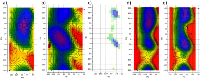
Accuracy of the force-field energy function with respect to backbone φ/ψ angles is of extraordinary importance in protein modeling because these angles determine secondary structure and because the relatively small angular deviations result in large movements as they propagate along the polypeptide chain. Therefore, we paid special attention to the parameters and choice of the functional form for φ/ψ torsion potentials. To gain initial understanding of the behavior of ICMFF force-field energy function, we calculated φ/ψ energy map (Fig. 2a) for the nonbonded terms (van der Waals and electrostatics) on the model molecule, Ac-Ala-NMe, and compared it to the QM energy map (Fig 2b). We also visualized the difference between the MM and QM energies as a heatmap on the φ/ψ plane, emphasizing areas populated in protein structures (Fig. 2c).

Figure 2.

(a) nonbonded plus electrostatics φ/ψ energy map for Ace-Ala-NMe; (b) QM φ/ψ energy map for Ace-Ala-NMe. The color code from purple to red corresponds to the 0–8 kcal/mol range; (c) heatmap of the deviations between the QM and MM (computed without torsion potential) energies for Ace-Ala-NMe. The size of the squares indicates the frequency (on a logarithmic scale) of occurrence of a particular φ/ψ value pair (within a 10°×10° bin); (d) Ramachandran plot for a set of 21 diverse ultra-high resolution structures (resolution between 0.5 and 0.8Å, PDBs 1ejg, 1ucs, 2vb1, 1us0, 2dsx, 1r6j, 2b97, 1x6z, 1gci, 1pq7, 1iua, 2ixt, 1w0n, 2h5c, 1nwz, 1n55, 2o9s, 2jfr, 2pwa, 2o7a and 2hs1), blue points. Background is colored by φ/ψ frequencies for a much broader protein set⁵³, calculated within each 10°×10° degrees square on the φ/ψ plane. (e) contour map of the φ/ψ torsion potential. Color code from purple to red corresponds to the 0–4 kcal/mol range; (f) final energy map including the torsion potential. The color code from purple to red corresponds to the 0–8 kcal/mol range.; (g) heatmap of the residual deviations between the QM and final MM energies for Ace-Ala-NMe. Size of the squares indicates the frequency (on a logarithmic scale) of occurrence of a particular φ/ψ value pair (within a 10°×10° bin). Contours in Fig. 2a,b,e,g are drawn with 1kcal/mol step.

Two regions on the φ/ψ energy map appeared to be significantly lower for the MM map as compared to the QM one: (1) the region below α′ and α_R, centered at approximately (φ = −120°,ψ = −60°); and (2) the region corresponding to β₂, centered at approximately (φ = −150°,ψ = 70°). Another deviating region was the horizontal stripe region following ψ~0°, where the MM energy is significantly higher. This difference is apparently due to some clashing of Nⁱ and Nⁱ⁺¹ backbone nitrogens. A comparison to the Ramachandran plot (Fig. 2d) suggests that these three discrepancies are true artifacts of the MM energy – indeed, the two areas where QM energy is significantly higher show low population in the Ramachandran plot, and, conversely, theψ ~ 0° region is well populated at least around φ ~ −90°.

To attenuate or eliminate these artifacts, we considered various functional forms of φ/ψ torsion potentials. Despite extensive efforts using various weighting schemes for fitting of traditional cosine potentials, including multiple harmonics (1–6) and sine/cosine combinations, we could not achieve satisfactory fit across the entire region of interest. A good fit for the characteristic minima points would invariably lead to ‘ripples’ elsewhere, resulting in an unsatisfactory overall profile. We eventually converged on a special functional form that introduces ‘a hump’ around specific φ/ψ value pair (see sub-section 1 of the Methods section). Use of the cosine-based function (eq. 5, 6) allowed us to evaluate the term quickly without additional trigonometric function calls because cosines of all torsions are calculated and stored anyway during geometry construction in ICM. We used two such ‘humps’, the first one of 4.0 kcal/mol at (φ = −120°,ψ = −60°) and second one of 2.0 kcal/mol at (φ = −150°,ψ = 70°), to compensate for the low-energy artifacts. The amplitudes of the two ‘humps’ were chosen to correct the E_α′ – E_C5 and E_β2 – E_C5 energy differences, respectively, to within 0.1 kcal/mol accuracy. C₅ rather than C₇^eq minimum was considered as a reference state because it is much more populated in protein structures and also because there are multiple indications that deep C₇^eq minimum might be an artifact of the QM calculations, associated with intramolecular hydrogen bonding. Indeed, a basis set superposition error (BSSE) results in the overestimation of the stabilization energy of hydrogen bonds by ab initio molecular orbital calculations.⁸⁴ BSSE can be corrected using counterpoise calculations, but for intramolecular hydrogen bonds this approach is not directly applicable. Another smaller effect is associated with stronger vibrational force constants of the more rigid, ring-like conformations held tight by the internal hydrogen bonds. The estimated contributions from these two effects are as high as 1.5–4.4 kcal/mol for the BSSE and ~0.3 kcal/mol for the vibrational effects.⁸⁵

A ψ-only two-cosine wave was used to compensate the high-energy artifact in the ψ~0°. region. However, we found that full compensation of the MM/QM difference in E_α – E_C5 led to an unsatisfactory geometry and excessive stability of the alpha-helical conformation in our tests for a 20-residue polyalanine peptide. We, therefore, reduced the amplitude of this component of the potential until average φ/ψ angle pairs in the energy minimized helix returned closer to typically observed values of φ = −60° and ψ = −45°. At the final amplitude of 1.4 kcal/mol, the minimum was at (φ= −66.2, ψ= −40.9). Importantly, when distance-dependent dielectric method rather than Colomb electrostatics is used, the average φ/ψ angles in the minimum were at (φ = −65.6°, ψ = −41.6°). It should be noted that this component of the torsion potential function affects directly the energy difference between alpha-helical and beta-strand conformations in a polypeptide. We are currently testing the force field in peptide folding simulations to fine-tune it in conjunction with other terms including the solvation model.

The contour map of the full φ/ψ torsion potential (Figure 2e) illustrates the corrections introduced into the MM energy: oval and round red/yellow areas are the two ‘humps’ while the blue/purple band is the ψ-only component. A contour map of the final total MM energy as well as the MM-QM difference heatmap are shown on Fig 2f and 2g, and the main minima of Ac-Ala-NMe are listed in Table 3. Good correspondence of the location and shape of the minima can be observed, in particular, in highly populated areas.

Ac-Gly-NMe

Glycine φ and ψ torsional parameters were obtained by fitting the ab initio map of terminally-blocked glycine with the corresponding MM map (Fig. 3). Several values of the weighting parameters c and c1 (0.0–2.0) from eq. 14 were considered with the best energy RMSD of 5.5 kcal/mol obtained for c = 0.5 and c₁ = 1.0. Figures 3a and 3b show the QM and MM energy maps of Ac-Gly-NMe with the latter computed using the optimized backbone torsional parameters. All the main features of the entire map are reproduced accurately. Notable differences include the shape and higher energy of the −30°<φ <30° region of the MM map, which is a result of the rigid internal geometry used. φ and ψ torsional parameters for glycine are given in Table S24.

Figure 3.

(a) QM and (b) MM maps for terminally blocked glycine. The color code from purple to red corresponds to the 0–20 kcal/mol range. Contours are drawn with 1kcal/mol step.

Ace-Pro-NMe

In contrast with other internal coordinate force fields, we also allowed flexibility of the φ angle in proline. While this torsion is commonly kept fixed in torsion space modeling because it is constrained by the proline’s pyrrolidine ring, deviations of up to 15–20° from the median value of −75° are frequently observed in X-ray protein structures (Figure 4). In the present version of the ICM force field we did not introduce any treatment of the internal flexibility of the proline ring, keeping internal variables of the side chain rigid. While this approach does result in somewhat distorted ring geometry when φ deviates far from the mean value, only minor distortions occur for φ angle values within the range of interest in protein simulations. Indeed, we compared the conformation of the ring atoms together with two adjacent backbone C atoms (of the proline itself and the preceding residue) for an idealized Ac-Pro-NMe conformation with φ angle fixed at −68.8 ± 20° before and after QM geometry optimization (HF6/31G**) and found that RMSD did not exceed 0.12 Å. We judged this an acceptable trade-off as compared to the much larger inaccuracies associated with completely rigid pyrrolidine ring.

Figure 4.

Histogram of the distribution of proline φ angle in 21 diverse ultra-high resolution protein structures (161 proline residues, average φ angle is −68.8°, see Legend to Fig. 2d).

We did not introduce any explicit torsional potential for the proline φ/ψ pair because the overall shape of the low-energy region was reproduced well by the non-bonded terms of the force field (Fig. 5). While the locations of the minima deviated somewhat from those observed in QM energy map (Fig. 5d,e), we judged that they may be influenced by the artifacts of QM calculations (see Ac-Ala-NMe section). Indeed, the reported experimental energy difference⁸⁶ between the cis- and trans- conformations of N-methylacetamide is 2.5 kcal/mol, which is much closer to our MM value of 2.7 kcal/mol than to the QM one of 3.89 kcal/mol (Table 4). Furthermore, the MM energy minima seem to correspond better with the Ramachandran plot for proline residue (Fig 5c).

Figure 5.

φ/ψ map for Ace-Pro-Nme: (a) QM energy map for trans-proline; (b) QM energy map for cis-proline; (c) Ramachandran map for trans- and cis-proline; (d) final MM energy map for trans-proline; (e) final MM energy map for cis-proline. The color code from purple to redof the energy maps corresponds to the 0–20 kcal/mol range. Contours are drawn with 1kcal/mol step

Table 4.

Backbone torsional angles and intramolecular energies for local minima of Ac-Pro-NMe optimized using QM (MP2/6-31G**+PCM//HF6-31G**) and MM (ICMFF) methods

conformer	ΔEQM, kcal/mol	φ, deg.	ψ, deg.	ω′, deg.	ΔEMM, kcal/mol	φ, deg.	ψ, deg.	ω′, deg.
1	0.00	−86.3	75.3	−172.9	0.00	−77.4	96.4	178.1
2	3.89	−91.0	−4.3	10.9	2.74	−80.8	−18.2	−2.6
3	7.18	−71.4	161.6	−3.1	3.78	−77.4	151.9	−1.0

3. Optimization of solvation parameters for loop modeling

The SA solvation model was optimized using a training set of conformations generated for 58 loops of 9 residues as described in the Methods Section. The goal of the optimization was to obtain the parameter set that would result in the most favorable ranking of the near-native solutions among a large number of decoy structures generated by the BPMC sampling. The rationale for this optimization is that the original parameters of the SA solvation model were derived by fitting to the vacuum/water transfer energies for small molecule analogues to aminoacid side-chains, which may not adequately capture some of the effects of the burial of a particular chemical moiety in the bulk protein interior.

The optimized solvation parameters are given in Table S25 of Supporting Information. A comparison with the initial parameter set (column 3, Table S25) shows that the optimization led to changes in all the parameters, although the most significant changes took place for aromatic carbon and oxygen and nitrogen atoms from ionized groups. Interestingly, the solvation parameter of aromatic carbon changed its sign, so the atom became hydrophobic rather than weakly hydrophilic as was the case in the original solvation model. The new sign of this parameter is in agreement with an empirical observation that aromatic side-chains have a strong tendency to be buried rather than exposed on the protein surface.

In principle, the optimized parameters are not guaranteed to be optimal, even for the training set of loops, because low-energy conformations, not found during the generation of the training set, may exist. Therefore, the quality of the parameters was first assessed for the same set of 9 residue loops by carrying out BPMC loop simulations. Average and median RMSD’s for the lowest-energy loop conformations produced by the new BPMC runs were in complete agreement with the corresponding values obtained at the end of the parameter optimization procedure, i.e., a global conformational search with the optimized solvation parameters did not locate any new low energy non-native conformations. This result can be attributed to the quality of the training set used in optimization and, therefore, to the efficiency of the search method that is able to explore thoroughly the conformational space of each loop.

Significant improvement over the results obtained with the initial solvation parameters was observed in both average and median RMSD’s. Thus, average RMSD decreased from 1.53 Å for the initial solvation model to 0.98 Å for the optimized set, whereas median RMSD dropped by 0.31 Å from 0.75 Å RMSD of the initial model.

To make sure that the optimized solvation parameters are transferable to loops of different lengths and indeed lead to better accuracy of loop predictions, calculations were also carried out for 7 and 11 residue loops using the original SA parameters and the optimized values. In agreement with the results obtained for the training set, the optimized solvation model led to better accuracy of the predictions for both loop lengths. The improvement was particularly significant for 11 residue loops where the average/median RMSD decreased from 2.26/1.64 Å for the initial set of parameters to 1.45/1.00 Å for the optimized solvation model. For 7 residue loops, the final average/median RMSD was 0.66/0.33 compared to 0.72/0.35 for the initial parameter set. Because longer loops are more exposed to the solvent, it could be expected that they should be more sensitive to the accuracy of the solvent model.

A comparison of the results obtained with the initial and optimized solvation models demonstrates that parameter optimization using a set of loop conformations and aimed at stabilizing native structure against a large number of decoys represents an efficient method to increase accuracy of a given force field and produces parameters transferable to loops of different lengths.

4. Loop modeling results

This section contains discussion of the results obtained for protein loops of 4-13 residues and can be roughly divided into three parts. First, we compare the general performance of two different internal coordinate force fields implemented in the ICM package, i.e, ECEPP/3, and the new force field, ICMFF, presented in this work. Performance of ICMFF is discussed in detail in the second part and compared to that of other methods reported in the literature in the last part.

Comparison of ECEPP/3 and ICMFF loop simulation results

The average and median RMSD’s computed for 4-11 residue loops with ECEPP/3 and for 4-13 residue loops with ICMFF are listed in Table 5. We did not carry out simulations with ECEPP/3 for the longest and the most time-consuming 12 and 13 residue loops. ICMFF performs better for the entire (4-11 residue) range of loop lengths with the average RMSD of more than 20% lower than for the ECEPP/3 force field.

Table 5.

Average and Median backbone RMSDs (Å) obtained with ICMFF and ECEPP/3.

Force field	Loop length	4	5	6	7	8	9	10	11	12	13
	Number of loops	34	115	100	81	62	58	40	19	30	28
ICMFF	Average	0.25	0.51	0.55	0.66	0.84	0.98	0.88	1.45	1.16	1.67
	Median	0.21	0.27	0.34	0.33	0.46	0.44	0.50	1.00	0.73	0.74
ECEPP/3	Average	0.36	0.66	0.67	0.81	1.31	1.60	1.34	1.88	-	-
	Median	0.33	0.45	0.44	0.49	0.73	0.89	0.74	1.53	-	-

RMSDs obtained with the two force fields grow almost linearly with loop length. Two small peaks in RMSD take place for 9 and 11 residue loops and are more pronounced for ECEPP/3 than for ICMFF. A similar trend, at least for the loops with less than 11 residues, can be observed in the results of Jacobson et al.⁶ Because the 4-11 residue loop sets used in this work are the same as those considered by Jacobson et al.,⁶ it is reasonable to suggest that the unexpectedly higher RMSD for 9 and 11 residue loops may be caused by some other feature of the set. For example, insufficient filtering could lead to a higher percentage of structures with lower experimental accuracy of the loop region. Unusual ionization states of the loop residues, or relatively close proximity of ligands or ions etc could also influence the outcome of the prediction.

Accuracy of the ICMFF-based loop predictions

A detailed examination of the ICMFF results showed that the predictions carried out for short loops (4-7 residues) are in general very accurate with only a few outliers (lowest energy structures with RMSD>2.0 Å). Thus, median RMSD is in the range of 0.2–0.4 Å which is comparable to the uncertainty of the experimental data. There are no outliers for 4 residue loops, i.e., RMSD never exceeds 0.6 Å. Despite the increase in the average RMSD for longer loops (8-10 residues), the accuracy of the predictions in terms of the median RMSD is still quite high (<0.5 Å). The loops containing 11 and 13 residues appear to be the most challenging for ab initio prediction as indicated by higher values of both average and median RMSD (Table 5). Examples of successful predictions obtained for 12-residue loop in 1oth and for 13-residue loop in 1p1m are given in Figures 6a and 6b.

Figure 6.

Overlay of the native (orange) structure and the lowest-energy (green) conformation predicted using ICMFF: (a) for the 12-residue loop in 1oth (residues 69-80); (b) for the 13-residue loop in 1p1m (residues 327-339); (c) for the 7-residue loop in 2rn2. The native loop conformation is stabilized by interactions with symmetric molecules (shown in gray); (d) for the 11-residue loop in 2eng. Red spheres represent water molecules stabilizing the native loop conformation.

Regarding the efficiency of the search algorithm, the results in Table 6 show that for short loops with up to 8 residues, there was only one sampling error, i.e., the situation where no conformation with the energy lower or equal to the energy of the optimized native loop was found (it occurred for one 7-residue loop). The percentage of sampling errors was still small (<6%) for 9-11 residue loops and increased considerably (>14%) for 12 residue loops. No sampling errors occurred for the longest 13 residue loops. A higher percentage of sampling errors for longer loops can be explained not only by the larger number of degrees of freedom but also by the fact that longer loops are usually located farther away from the body of the protein. This leads to the much larger size of the conformational space to be explored because loop conformations are less influenced by the interactions with the rest of the protein. Second, on average, the solvent exposure of a loop grows with the length resulting in the higher sensitivity of the result to the accuracy of the solvation model used.

Table 6.

Percentage of error attributable to sampling

Loop length	4	5	6	7	8	9	10	11	12	13
Percentage of error (%)	0	0	0	1	0	2	3	6	14	0

In general, the number of poorly predicted loops (i.e., those with RMSD greater than 2 Å) increases gradually with loop length. Thus, the percentage of incorrect predictions is 0% for 4-residue loops, 12% for 7 residue loops, ~20% for 11 and 12-residue loops, and reaches a maximum of 32% for 13-residue loops. Only one incorrect prediction has energy higher than that of the corresponding optimized native conformation and, therefore, can be explained by a sampling error. To study the origin of all other incorrect predictions, we carried out structural analysis of the corresponding experimental structures. In particular, we were looking for close (< 4 Å) contacts between heavy atoms of the loop and any crystallographic neighbor of the protein molecule. Close intermolecular contacts were found in ~76% of cases with many of them involving hydrogen bonds. This result suggests that crystal packing may have significant influence on loop conformations for the cases with high predicted RMSD. Fig. 6c showing the lowest-energy predicted loop conformation for 2rn2 (7-residue loop) overlaid with the corresponding native structure illustrates the effect of crystal packing on the outcome of the loop simulations.

The remaining wrong predictions may be caused by a number of reasons. As mentioned above, highly solvent-exposed loops are more sensitive to the correct balance of intramolecular and solvation energy contributions. An example of this situation is shown in Fig. 6d for the 11 residue loop in 2eng. This is a particularly interesting case because this loop is packed inside a cavity but with a layer of water molecules separating it from the rest of the protein. An explicit water model may be necessary for correct prediction of this loop.

Other possible factors that may affect the prediction outcome include minor defects of the experimental structures in the vicinity of the loop, as well as uniform protonation state assignment (corresponding to pH 7) regardless of the actual pH of the experiment and local structure environment.

Results obtained for the two loops containing cis-proline [lowest-energy conformations with RMSD of 0.39 and 0.27 Å for 1w0n and 2ixt, respectively (Table S11 and S14, Supporting Information)] demonstrated that the ICMFF description of the internal energy of proline residue is accurate enough to reproduce the energetic balance between trans- and cis-isomers. Figure 7 shows the overlay of the native and the lowest-energy predicted conformations of the 178–186 loop in 2ixt.

Figure 7.

Overlay of the native (orange) structure and the lowest-energy (green) conformation predicted using ICMFF for the 9-residue loop containing cis-proline (2ixt, residues 69-80).

Comparison with previously published methods

In most cases, a comparison of our results with the previous studies is confounded by the differences in the composition of the test sets and the inclusion of crystallographic neighbors in loop modeling in other studies. However, results reported by Sellers et al.⁵ for 6, 8, 10, and 12 residue loops can be compared directly with those discussed in this work because they were obtained without considering the crystal environment. Moreover, our loop sets contain, among others, all the loops used by Sellers et al. We plotted the percentage of loops with RMSD below a given cutoff as a function of the cutoff computed based on the results of Sellers et al. (taken from Table S5 in Ref.5) and those reported in this work for 6, 8, 10, and 12 residue loops (Figure 8a–d). For shorter loops (6 and 8 residues), performance of ICM in clearly superior to that of HLP in terms of average RMSD and very close in terms of median RMSD [average/median RMSD for 6 residue loops is 0.7/0.3 Å for HLP and 0.4/0.3 Å for ICM; RMSD for 8-residue loops is 1.2/0.6 Å for HLP and 0.5/0.5 Å for ICM (Table 7)]. For 10 residue loops, ICM performs somewhat worse than HLP mainly because of the larger number of outliers as indicated by a higher average (0.8 Å versus 0.6 Å for ICM and HLP, respectively) and almost identical median RMSD (0.5 Å versus 0.4 Å for ICM and HLP, respectively). Both ICM and HLP methods behave very similarly for 12 residue loops, with an average RMSD of 1.1 and 1.2 Å and a median RMSD of 0.7 and 0.6 Å, respectively. It should be mentioned that the size of the loop sets used for this comparison is relatively small (20 loops for each length) and therefore, the 0.1–0.2 Å difference in RMSD may not be statistically significant.

Figure 8.

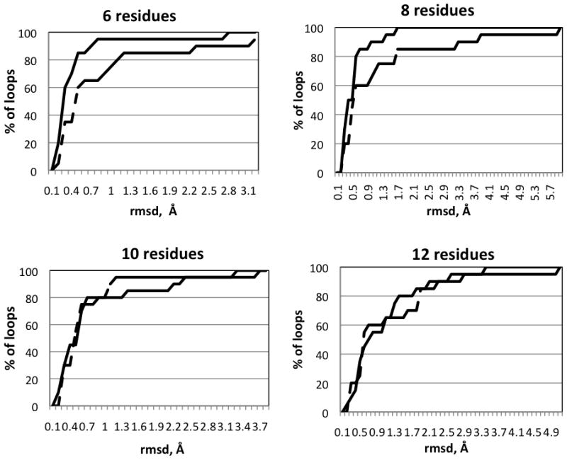
Comparison of loop prediction results obtained with ICM (solid line) and reported⁵ for HLP (dashed line). The y-axis is the percentage of loops for which the backbone RMSD of the lowest-energy conformation is at or below the RMSD on the x-axis.

Table 7.

Comparison of the ICMFF loop prediction results with published works.

Loop length	RMSD	6	8	10	12	13
ICM	average	0.4	0.5	0.8	1.1	1.67
	median	0.4	0.5	0.5	0.7	0.74
HLPf	average	0.7	1.2	0.6	1.2	na
	median	0.3	0.6	0.4	0.6	na
PLOP IIh	average	na	na	na	1.15	1.28
	median	na	na	na	0.60	0.72

^fData taken from Table I of Sellers et al.⁵

^hData taken from Table II of Zhu et al.⁴ 1hxh and 1dpg from the original loop set were not considered in this work because these proteins are biological tetramer and dimer, respectively, with large interfaces in the loops regions. RMSD values for PLOP II were computed using data from Table II of Zhu et al.⁴

Results obtained here for 13 residue loops can be compared directly to those of Zhu et al.⁴ because the same set of loops was considered in both studies. The average RMSD of our predictions is ~30% higher than that of Zhu et al. (1.67 Å vs. 1.28 Å, Table 7); however, the median RMSD’s are virtually identical for both methods (0.74 and 0.72 for ICMFF and PLOP II, respectively). The analysis of our results for each loop showed that there are three outliers (1hnj, 1jp4, 1ojq) with RMSD greater than 4 Å. In all three cases, the loop residues form multiple close contacts with crystallographic neighbors. Zhu et al.⁴ reconstructed the crystal packing (an asymmetric unit plus all atoms from the surrounding symmetric units within 30 Å) in their simulation, which likely helped their method to predict native-like loop conformations for all three proteins.

ICMFF is an internal coordinate force field and as such it relies on the use of standard bond lengths and bond angles (except ∠NC^αC). It is reasonable to ask whether the fixed standard residue geometry has any significant effect on the accuracy of the loop modeling. If such an effect exists, it can be expected to be more noticeable for the shortest loops (whereas, for longer loops the errors may be obscured by the noise from nonbonded interactions or may compensate each other). The comparison (in terms of median RMSD) with the highly accurate results reported by Jacobson et al.⁶ for 4, 5 residue loops and by Sellers et al.⁵ for 6 residue loops indicates that rigid geometry approximation, at least when it is used in combination with an accurate force field and relaxation of ∠NC^αC angle, can provide accuracy of loop predictions which is as good as that of high quality Cartesian potentials. Thus, the same median RMSD of 0.2 Å was obtained for 4 residue loops with ICMFF and reported by Jacobson et al. Both ICM and HLS⁵ yielded median RMSD of 0.3 Å for 6 residue loops.

As pointed out by Chen at el.,⁶² rigid covalent geometry in torsion space modeling affects not only the profile of the low energy regions (which we correct by an appropriate torsion potential) but also the height of the barriers between them. Higher barriers are a significant issue in torsion angle molecular dynamics, and special torsion cross-term corrections have been proposed to recover the potential surface across both, low- and high- energy regions.⁶² In Monte-Carlo minimization simulations, where the main goal is to explore the low-energy minima, the barriers issue appears to be rather minor because the search procedure is able to ‘jump’ from one low energy region to another irrespective of the height of the barrier. Furthermore, introduction of the flexibility of ∠NC^αC planar angle in ICMFF reduces the barriers for backbone flexing: indeed, the lowest saddle points on φ = 0° (ψ ~ 90°) and ψ = 0° (φ ~ −90°) rotation barriers are lowered by 6.0 kcal/mol and 0.8 kcal/mol, respectively, as compared to rigid ∠NC^αC model. These lower barriers may further ease the sampling of various backbone conformations.

5. Computational cost

All loop simulations were carried out on a cluster of Intel Core2 processors at 2.13 GHz. The average CPU time per single run is 2.5 h for 8-residue loop; 12 h for 10-residue loop and 55 h for 12-residue loop. A sharp increase in computational time with the number of residues in the loop is due to the exponential dependence of the number of energy evaluations required for adequate sampling of the conformational space at the second stage of our protocol. We are currently developing an improved version of the loop modeling algorithm that will be characterized by a more efficient sampling at the first stage and, therefore, will enable us to decrease significantly the number of energy evaluations required for the second, more time consuming stage.

The results reported in this work were obtained by performing five independent runs for each loop. All five runs can be performed simultaneously on a cluster or even on multiple CPU cores of a single workstation.

Conclusions

Loop simulations represent a rigorous test of the force-field accuracy and the sampling method, and are important for many practical applications such as homology modeling and protein design. A comparison with other studies shows that the ICM loop modeling method provides high accuracy of predictions and is on par with the most accurate methods developed so far. Success in loop modeling simulations also provides the first demonstration of the quality of our novel torsion force field, ICMFF. Further tests including energy ranking of protein decoys or folding of small proteins and peptides are necessary for more comprehensive evaluation of the force field. We are planning to carry these test out in the future.

References

- 1.Berman HM, Westbrook J, Feng Z, Gilliland G, Bhat TN, Weissig H, Shindyalov IN, Bourne PE. The Protein Data Bank. Nucleic Acids Res. 2000;28(1):235–242. doi: 10.1093/nar/28.1.235. [DOI] [PMC free article] [PubMed] [Google Scholar]
- 2.Chothia C, Lesk AM. Canonical structures for the hypervariable regions of immunoglobulins. J Mol Biol. 1987;196(4):901–917. doi: 10.1016/0022-2836(87)90412-8. [DOI] [PubMed] [Google Scholar]
- 3.Chothia C, Lesk AM, Tramontano A, Levitt M, Smith-Gill SJ, Air G, Sheriff S, Padlan EA, Davies D, Tulip WR, et al. Conformations of immunoglobulin hypervariable regions. Nature. 1989;342(6252):877–883. doi: 10.1038/342877a0. [DOI] [PubMed] [Google Scholar]
- 4.Zhu K, Pincus DL, Zhao S, Friesner RA. Long loop prediction using the protein local optimization program. Proteins. 2006;65(2):438–452. doi: 10.1002/prot.21040. [DOI] [PubMed] [Google Scholar]
- 5.Sellers BD, Zhu K, Zhao S, Friesner RA, Jacobson MP. Toward better refinement of comparative models: predicting loops in inexact environments. Proteins. 2008;72(3):959–971. doi: 10.1002/prot.21990. [DOI] [PMC free article] [PubMed] [Google Scholar]
- 6.Jacobson MP, Pincus DL, Rapp CS, Day TJ, Honig B, Shaw DE, Friesner RA. A hierarchical approach to all-atom protein loop prediction. Proteins. 2004;55(2):351–367. doi: 10.1002/prot.10613. [DOI] [PubMed] [Google Scholar]
- 7.Xiang Z, Soto CS, Honig B. Evaluating conformational free energies: the colony energy and its application to the problem of loop prediction. Proc Natl Acad Sci U S A. 2002;99(11):7432–7437. doi: 10.1073/pnas.102179699. [DOI] [PMC free article] [PubMed] [Google Scholar]
- 8.Danielson ML, Lill MA. New computational method for prediction of interacting protein loop regions. Proteins: Structure, Function, Bioinformatics. 2010 doi: 10.1002/prot.22690. [DOI] [PubMed] [Google Scholar]
- 9.Fiser A, Do RK, Sali A. Modeling of loops in protein structures. Protein Sci. 2000;9(9):1753–1773. doi: 10.1110/ps.9.9.1753. [DOI] [PMC free article] [PubMed] [Google Scholar]
- 10.Soto CS, Fasnacht M, Zhu J, Forrest L, Honig B. Loop modeling: Sampling, filtering, and scoring. Proteins. 2008;70(3):834–843. doi: 10.1002/prot.21612. [DOI] [PMC free article] [PubMed] [Google Scholar]
- 11.Wojcik J, Mornon JP, Chomilier J. New efficient statistical sequence-dependent structure prediction of short to medium-sized protein loops based on an exhaustive loop classification. J Mol Biol. 1999;289(5):1469–1490. doi: 10.1006/jmbi.1999.2826. [DOI] [PubMed] [Google Scholar]
- 12.van Vlijmen HW, Karplus M. PDB-based protein loop prediction: parameters for selection and methods for optimization. J Mol Biol. 1997;267(4):975–1001. doi: 10.1006/jmbi.1996.0857. [DOI] [PubMed] [Google Scholar]
- 13.Michalsky E, Goede A, Preissner R. Loops In Proteins (LIP)--a comprehensive loop database for homology modelling. Protein Eng. 2003;16(12):979–985. doi: 10.1093/protein/gzg119. [DOI] [PubMed] [Google Scholar]
- 14.Shenkin PS, Yarmush DL, Fine RM, Levinthal C. Method for quickly generating random conformations of ring-like structures for subsequent energy minimization or molecular-dynamics - application to antibody hypervariable loops. Biophysical Journal. 1987;51:A232–A232. [Google Scholar]
- 15.Galaktionov S, Nikiforovich GV, Marshall GR. Ab initio modeling of small, medium, and large loops in proteins. Biopolymers. 2001;60(2):153–168. doi: 10.1002/1097-0282(2001)60:2<153::AID-BIP1010>3.0.CO;2-6. [DOI] [PubMed] [Google Scholar]
- 16.Dudek MJ, Scheraga HA. Protein-structure prediction using a combination of sequence homology and global energy minimization. 1. Global energy minimization of surface loops. Journal of Computational Chemistry. 1990;11:121–151. [Google Scholar]
- 17.Palmer KA, Scheraga HA. Standard-geometry chains fitted to x-ray derived structures -validation of the rigid-geometry approximation. 2. Systematic searches for short loops in proteins - applications to bovine pancreatic ribonuclease-A and human lysozyme. Journal of computational chemistry. 1992;13:329–350. [Google Scholar]
- 18.Das B, Meirovitch H. Optimization of solvation models for predicting the structure of surface loops in proteins. Proteins. 2001;43(3):303–314. doi: 10.1002/prot.1041. [DOI] [PubMed] [Google Scholar]
- 19.Bruccoleri RE, Karplus M. Prediction of the folding of short polypeptide segments by uniform conformational sampling. Biopolymers. 1987;26(1):137–168. doi: 10.1002/bip.360260114. [DOI] [PubMed] [Google Scholar]
- 20.Rapp CS, Friesner RA. Prediction of loop geometries using a generalized born model of solvation effects. Proteins. 1999;35(2):173–183. [PubMed] [Google Scholar]
- 21.Deane CM, Blundell TL. A novel exhaustive search algorithm for predicting the conformation of polypeptide segments in proteins. Proteins. 2000;40(1):135–144. [PubMed] [Google Scholar]
- 22.DePristo MA, de Bakker PI, Lovell SC, Blundell TL. Ab initio construction of polypeptide fragments: efficient generation of accurate, representative ensembles. Proteins. 2003;51(1):41–55. doi: 10.1002/prot.10285. [DOI] [PubMed] [Google Scholar]
- 23.Deane CM, Blundell TL. CODA: a combined algorithm for predicting the structurally variable regions of protein models. Protein Sci. 2001;10(3):599–612. doi: 10.1110/ps.37601. [DOI] [PMC free article] [PubMed] [Google Scholar]
- 24.Zhang H, Lai L, Wang L, Han Y, Tang Y. A fast and efficient program for modeling protein loops. Biopolymers. 1999;41:61–72. [Google Scholar]
- 25.McGarrah DB, Judson RS. Analysis of the genetic algorithm method of molecular conformation determination. Journal of computational chemistry. 1993;14:1385–1395. [Google Scholar]
- 26.Ring CS, Cohen FE. Conformational sampling of loop structures using genetic algorithms. Israeli journal of chemistry. 1994;34:245–252. [Google Scholar]
- 27.Moult J, James MN. An algorithm for determining the conformation of polypeptide segments in proteins by systematic search. Proteins. 1986;1(2):146–163. doi: 10.1002/prot.340010207. [DOI] [PubMed] [Google Scholar]
- 28.Shenkin PS, Yarmush DL, Fine RM, Wang HJ, Levinthal C. Predicting antibody hypervariable loop conformation. I. Ensembles of random conformations for ringlike structures. Biopolymers. 1987;26(12):2053–2085. doi: 10.1002/bip.360261207. [DOI] [PubMed] [Google Scholar]
- 29.Go N, Scheraga HA. Ring closure and local conformation deformations of chain molecules. Macromolecules. 1970;3:178–187. [Google Scholar]
- 30.Wedemeyer W, Scheraga HA. Exact analytical loop closure in proteins using polynomial equations. Journal of computational chemistry. 1999;20:819–844. doi: 10.1002/(SICI)1096-987X(199906)20:8<819::AID-JCC8>3.0.CO;2-Y. [DOI] [PubMed] [Google Scholar]
- 31.Bruccoleri RE, Karplus M. Chain closure with bond angle variations. Macromolecules. 1985;18:2767–2773. [Google Scholar]
- 32.de Bakker PI, DePristo MA, Burke DF, Blundell TL. Ab initio construction of polypeptide fragments: Accuracy of loop decoy discrimination by an all-atom statistical potential and the AMBER force field with the Generalized Born solvation model. Proteins. 2003;51(1):21–40. doi: 10.1002/prot.10235. [DOI] [PubMed] [Google Scholar]
- 33.Zhang C, Liu S, Zhou Y. Accurate and efficient loop selections by the DFIRE-based all-atom statistical potential. Protein Sci. 2004;13(2):391–399. doi: 10.1110/ps.03411904. [DOI] [PMC free article] [PubMed] [Google Scholar]
- 34.Rata IA, Li Y, Jakobsson E. Backbone Statistical Potential from Local Sequence-Structure Interactions in Protein Loops. Journal of Physical Chemistry B. 2010;114:1859–1869. doi: 10.1021/jp909874g. [DOI] [PubMed] [Google Scholar]
- 35.Rohl CA, Strauss CE, Chivian D, Baker D. Modeling structurally variable regions in homologous proteins with rosetta. Proteins. 2004;55(3):656–677. doi: 10.1002/prot.10629. [DOI] [PubMed] [Google Scholar]
- 36.Olson MA, Feig M, Brooks CL., 3rd Prediction of protein loop conformations using multiscale modeling methods with physical energy scoring functions. J Comput Chem. 2008;29(5):820–831. doi: 10.1002/jcc.20827. [DOI] [PubMed] [Google Scholar]
- 37.Das B, Meirovitch H. Solvation parameters for predicting the structure of surface loops in proteins: transferability and entropic effects. Proteins. 2003;51(3):470–483. doi: 10.1002/prot.10356. [DOI] [PubMed] [Google Scholar]
- 38.Felts AK, Gallicchio E, Chekmarev D, Paris KA, Friesner RA, Levy RM. Prediction of Protein Loop Conformations using the AGBNP Implicit Solvent Model and Torsion Angle Sampling. J Chem Theory Comput. 2008;4(5):855–868. doi: 10.1021/ct800051k. [DOI] [PMC free article] [PubMed] [Google Scholar]
- 39.Smith KC, Honig B. Evaluation of the conformational free energies of loops in proteins. Proteins. 1994;18(2):119–132. doi: 10.1002/prot.340180205. [DOI] [PubMed] [Google Scholar]
- 40.Abagyan R, Totrov M, Kuznetsov D. ICM - a new method for protein modeling and design - applications to docking and structure prediction from the distorted native conformation. Journal of computational chemistry. 1994;15:488. [Google Scholar]
- 41.Scheraga HA. Calculations of conformations of polypeptides. Adv Phys Org Chem. 1971;71:195. [Google Scholar]
- 42.Némethy G, Gibson KD, Palmer KA, Yoon CN, Paterlini G, Zagari A, Rumsey S, Scheraga HA. Energy parameters in polypeptides. 10 Improved geometrical parameters and nonbonded interactions for use in the ECEPP/3 algorithm, with application to praline-containing peptides. Journal of physical chemistry. 1992;96:6472. [Google Scholar]
- 43.Vila JA, Ripoll DR, Scheraga HA. Atomically detailed folding simulation of the B domain of staphylococcal protein A from random structures. Proc Natl Acad Sci U S A. 2003;100(25):14812–14816. doi: 10.1073/pnas.2436463100. [DOI] [PMC free article] [PubMed] [Google Scholar]
- 44.Ripoll DR, Vila JA, Scheraga HA. Folding of the villin headpiece subdomain from random structures. Analysis of the charge distribution as a function of pH. J Mol Biol. 2004;339(4):915–925. doi: 10.1016/j.jmb.2004.04.002. [DOI] [PubMed] [Google Scholar]
- 45.Vila JA, Ripoll DR, Arnautova YA, Vorobjev YN, Scheraga HA. Coupling between conformation and proton binding in proteins. Proteins. 2005;61(1):56–68. doi: 10.1002/prot.20531. [DOI] [PubMed] [Google Scholar]
- 46.Arnautova YA, Jagielska A, Scheraga HA. A new force field (ECEPP-05) for peptides, proteins, and organic molecules. Journal of Physical chemistry B. 2006;110:5025–5044. doi: 10.1021/jp054994x. [DOI] [PubMed] [Google Scholar]
- 47.Arnautova YA, Vorobjev YN, Vila JA, Scheraga HA. Identifying native-like protein structures with scoring functions based on all-atom ECEPP force fields, implicit solvent models and structure relaxation. Proteins. 2009;77(1):38–51. doi: 10.1002/prot.22414. [DOI] [PMC free article] [PubMed] [Google Scholar]
- 48.Totrov M, Abagyan R. Flexible protein-ligand docking by global energy optimization in internal coordinates. Proteins. 1997;(Suppl 1):215–220. doi: 10.1002/(sici)1097-0134(1997)1+<215::aid-prot29>3.3.co;2-i. [DOI] [PubMed] [Google Scholar]
- 49.Abagyan R, Totrov M. High-throughput docking for lead generation. Curr Opin Chem Biol. 2001;5(4):375–382. doi: 10.1016/s1367-5931(00)00217-9. [DOI] [PubMed] [Google Scholar]
- 50.Berkholz DS, Shapovalov MV, Dunbrack RL, Jr, Karplus PA. Conformation dependence of backbone geometry in proteins. Structure. 2009;17(10):1316–1325. doi: 10.1016/j.str.2009.08.012. [DOI] [PMC free article] [PubMed] [Google Scholar]
- 51.Schafer L, Cao M. Predictions of protein backbone bond distances and angles from first principles. Journal of molecular structure. 1995;333:201–208. [Google Scholar]
- 52.Karplus PA. Experimentally observed conformation-dependent geometry and hidden strain in proteins. Protein Sci. 1996;5(7):1406–1420. doi: 10.1002/pro.5560050719. [DOI] [PMC free article] [PubMed] [Google Scholar]
- 53.Abagyan R, Totrov M. Biased probability Monte Carlo conformational searches and electrostatic calculations for peptides and proteins. J Mol Biol. 1994;235(3):983–1002. doi: 10.1006/jmbi.1994.1052. [DOI] [PubMed] [Google Scholar]
- 54.Abagyan RA, Totrov M. Ab initio folding of peptides by the optimal-bias Monte Carlo minimization procedure. Journal of computational physics. 1999;151:402–421. [Google Scholar]
- 55.Cardozo T, Totrov M, Abagyan R. Homology modeling by the ICM method. Proteins. 1995;23(3):403–414. doi: 10.1002/prot.340230314. [DOI] [PubMed] [Google Scholar]
- 56.Abagyan R, Batalov S, Cardozo T, Totrov M, Webber J, Zhou Y. Homology modeling with internal coordinate mechanics: deformation zone mapping and improvements of models via conformational search. Proteins. 1997;(Suppl 1):29–37. doi: 10.1002/(sici)1097-0134(1997)1+<29::aid-prot5>3.3.co;2-4. [DOI] [PubMed] [Google Scholar]
- 57.Jagielska A, Arnautova YA, Scheraga HA. Derivation of a new force field for crystal-structure prediction using global optimization: nonbonded potential parameters for amines, imidazoles, amides, and carboxylic acids. Journal of Physical chemistry B. 2004;108:12181–12196. [Google Scholar]
- 58.Filippini G, Gavezzotti A. Empirical intermolecular potentials for organic crystals: the ‘6-exp’ approximation revisited. Acta Crystallogr B. 1993;49:868–880. [Google Scholar]
- 59.Mackerell AD, Jr, Feig M, Brooks CL., 3rd Extending the treatment of backbone energetics in protein force fields: limitations of gas-phase quantum mechanics in reproducing protein conformational distributions in molecular dynamics simulations. J Comput Chem. 2004;25(11):1400–1415. doi: 10.1002/jcc.20065. [DOI] [PubMed] [Google Scholar]
- 60.MacKerell AD, Jr, Feig M, Brooks CL., 3rd Improved treatment of the protein backbone in empirical force fields. J Am Chem Soc. 2004;126(3):698–699. doi: 10.1021/ja036959e. [DOI] [PubMed] [Google Scholar]
- 61.Feig MM, AD, Brooks CL., 3rd Force field influence on the observation of pi-helical protein structures in molecular dynamics simulations. Journal of physical chemistry. 2003;B107:2831–2836. [Google Scholar]
- 62.Chen J, Im W, Brooks CL., 3rd Application of torsional angles molecular dynamics for efficient sampling of protein conformations. Journal of computational chemistry. 2005;26:1565–1578. doi: 10.1002/jcc.20293. [DOI] [PubMed] [Google Scholar]
- 63.Allen FH, Kennard O, Taylor R. Systematic analysis of structural data as a research technique in organic chemistry. Accounts of chemical research. 1983;16:146–153. [Google Scholar]
- 64.Chickos JS. Heat of Sublimation Data. In: Linstrom PJ, Mallard WG, editors. NIST Chemistry WebBook, NIST Standard Reference Database Number 69. National Institute of Standards and Technology; Gaithersburg MD: p. 20899. http://webbooknistgov, (retrieved June 1, 2009) [Google Scholar]
- 65.Bondi A. Heat of sublimation of molecular crystals: a catalog of molecular structure increments. Journal of chemical and engineering data. 1963;8:371–381. [Google Scholar]
- 66.Pillardy J, Arnautova YA, Czaplewski C, Gibson KD, Scheraga HA. Conformation-family Monte Carlo: a new method for crystal structure prediction. Proc Natl Acad Sci U S A. 2001;98(22):12351–12356. doi: 10.1073/pnas.231479298. [DOI] [PMC free article] [PubMed] [Google Scholar]
- 67.Desiraju GR, Steiner T, editors. The weak hydrogen bond in structural chemistry and biology. Oxford University Press; Oxford: 1999. p. 507. [Google Scholar]
- 68.Bondi A. van der Waals volumes and radii. Journal of Physical Chemistry. 1964;68(3):441–451. [Google Scholar]
- 69.Head-Gordon M, Pople JA, Frisch MJ. MP2 energy evaluation by direct methods. Chem Phys Lett. 1988;153:503–506. [Google Scholar]
- 70.Frisch MJ, Head-Gordon M, Pople JA. A direct MP2 gradient method. Chemical Physics Letters. 1990;166(3):275–280. [Google Scholar]
- 71.Schmidt MW, Baldridge KK, Boatz JA, Elbert ST, Gordon MS, Jensen JH, Koseki S, Matsunaga N, Nguyen KA, Su S, Windus TL, Dupuis M, Montgomery JA. General Atomic and Molecular Electronic Structure System. Journal of computational chemistry. 1993;14:1347–1363. [Google Scholar]
- 72.Gordon MS, Schmidt MW. Advances in electronic structure theory: GAMESS a decade later. In: Dykstra CE, Frenking G, Kim KS, Scuseria GE, editors. Theory and Applications of Computational Chemistry: the first forty years. Elsevier; Amsterdam: 2005. pp. 1167–1189. [Google Scholar]
- 73.Abagyan RA. Protein structure prediction by global energy optimization. In: van Gunsteren WF, et al., editors. Computer Simulation of biomolecular systems. Vol. 3. Kluwer/Escom; London: 1997. p. 363. [Google Scholar]
- 74.Press WH, Teukolsky SA, Vetterling WT, Flannery BP. Numerical recipes in Fortran 77: the art of scientific computing. Cambridge; New York: Cambridge University Press; 2000. [Google Scholar]
- 75.Gavezzotti A. Theoretical aspects and computer modelling of the molecular solid state. John Wiley & sons; Chichester: 1997. [Google Scholar]
- 76.van de Streek J, Verwer P, Bennema P, Vlieg E. On the influence of thermal motion on the crystal structures and polymorphism of even n-alkanes. Acta Crystallogr B. 2002;58(Pt 4):677–683. doi: 10.1107/s0108768102004147. [DOI] [PubMed] [Google Scholar]
- 77.van de Streek J, Verwer P, Bennema P, Vlieg E. On the irrelevance of electrostatics for the crystal structures and polymorphism of long even n-alkanes. J Comput Chem. 2002;23(3):365–370. doi: 10.1002/jcc.10028. [DOI] [PubMed] [Google Scholar]
- 78.Coombes DS, Price SL, Willock DJ, Leslie M. Role of electrostatic interactions in determining the crystal structures of polar organic molecules. A distributed multipole study. Journal of Physical Chemistry. 1996;100:7352–7360. [Google Scholar]
- 79.Mooij W, van Eijck B, Price S, Verwer P, Kroon J. Crystal structure predictions for acetic acid. Journal of Computational Chemistry. 1998;19:459–474. [Google Scholar]
- 80.Mitchell JBO, Price SL. A systematic nonempirical method of deriving model intermolecular potentials for organic molecules: Application to amides. Journal of Physical Chemistry A. 2000;104(46):10958–10971. [Google Scholar]
- 81.Abraha A, Williams DE. Spherical and Aspherical Intermolecular Force Fields for Sulfur Allotropes. Inorganic Chemistry. 1999;38:4224–4228. [Google Scholar]
- 82.Day GM, Price SL, Leslie M. Atomistic calculations of phonon frequencies and thermodynamic quantities for crystals of rigid organic molecules. Journal of Physical Chemistry B. 2003;107:10919–10933. [Google Scholar]
- 83.Lovell SC, Word JM, Richardson JS, Richardson DC. The penultimate rotamer library. Proteins. 2000;40(3):389–408. [PubMed] [Google Scholar]
- 84.van Duijneveldt FB. Basis set superposition error. In: Scheiner S, editor. Molecular Interactions. Wiley; Chichester, UK: 1997. p. 81. [Google Scholar]
- 85.Tsai MI, Xu Y, Dannenberg JJ. Ramachandran revisited. DFT energy surfaces of diastereomeric trialanine peptides in the gas phase and aqueous solution. J Phys Chem B. 2009;113(1):309–318. doi: 10.1021/jp8063646. [DOI] [PubMed] [Google Scholar]
- 86.Drakenbe T, Forsen S. Barrier to internal rotation in monosubstituted amides. Journal of the Chemical Society D, Chemical Communications. 1971;(21):1404. [Google Scholar]
Associated Data
This section collects any data citations, data availability statements, or supplementary materials included in this article.