Managing ecological thresholds in coupled environmental–human systems

Abstract

Many ecosystems appear subject to regime shifts—abrupt changes from one state to another after crossing a threshold or tipping point. Thresholds and their associated stability landscapes are determined within a coupled socioeconomic–ecological system (SES) where human choices, including those of managers, are feedback responses. Prior work has made one of two assumptions about managers: that they face no institutional constraints, in which case the SES may be managed to be fairly robust to shocks and tipping points are of little importance, or that managers are rigidly constrained with no flexibility to adapt, in which case the inferred thresholds may poorly reflect actual managerial flexibility. We model a multidimensional SES to investigate how alternative institutions affect SES stability landscapes and alter tipping points. With institutionally dependent human feedbacks, the stability landscape depends on institutional arrangements. Strong institutions that account for feedback responses create the possibility for desirable states of the world and can cause undesirable states to cease to exist. Intermediate institutions interact with ecological relationships to determine the existence and nature of tipping points. Finally, weak institutions can eliminate tipping points so that only undesirable states of the world remain.

Ecological multistability theory describes how distinct ecosystems, identical but for their initial states, can stabilize at very different long-run equilibria. A costly or irreversible “regime shift” can subsequently occur when a multistable (MS) system is moved past a threshold or tipping point and into an alternative equilibrium's basin of attraction (1–3) (Fig. 1). The management of MS systems has become a focal point of the science–policy interface (4–6) in response to fisheries collapse, climate change, vegetation changes, and invasive species, as these phenomena are often deemed causes and effects of regime shifts that reduce ecosystem services (7).

Fig. 1.

Types of regime shifts, based on Beisner et al. (3). The ball represents an ecological system, and the basins represent equilibria: If a ball is dropped, it will settle in a basin. (A) Regime shift due to a “shift in variables.” Here, a force that is external to the dynamic system (e.g., an exogenous shock or perturbation) pushes the system across a fixed threshold and into a new basin. (B) Regime shift due to a “shift in parameters.” Here, a change in a parameter of the dynamic system (e.g., carrying capacity, death rate) alters the topology of the system (i.e., the “shape” of the dynamic system, defining thresholds and basins of attraction) so that the system moves into the new basin.

Increasingly, human-impacted ecological systems, including MS systems, are regarded as coupled socioeconomic–ecological systems (SES) where human behaviors are feedback responses affecting, and affected by, ecological variables (8) (Fig. 2). The SES perspective means that solving ecological problems requires altering the SES's stability landscape or topology (i.e., the dynamic system's “shape”, defining thresholds and basins of attraction) so the system moves to a preferred outcome (8, 9). This result is achieved by imposing regulations or altering economic signals that influence human feedback responses (Fig. 2). An ensuing regime shift might be said to result from a shift in regulatory institutions, extending Beisner et al.’s (3) categorization (Fig. 1).

Fig. 2.

A conceptual framework for the SES. Here thresholds shift in response to management policies affecting human feedback responses. A feedback response means the state of the ecological system affects economic signals that resource managers and anglers respond to. Foresighted managers predict current and future ecological and economic impacts when making policy choices. Managers and anglers respond differently to different institutional settings (i.e., the set of policies used by managers and the resources available to managers for direct manipulation), resulting in different feedback processes and topologies.

SES management is often modeled using a bioeconomic framework that combines economic decision theory with ecological modeling (10). Work on MS-SESs has focused on problems such as rangeland ecosystems (9, 11), coral reefs (12), fisheries (13), and nutrients in shallow lakes (14, 15). In these models, foresighted managers direct the system along a well-defined approach path to a particular stable outcome (assuming a stationary system). Managers will find it desirable to adjust policy variables to pursue the same stable, long-run outcome for a range of initial ecological states, defining an SES basin of attraction. SES stability means that, if a shock occurs and does not move the system outside this basin, managers will find it beneficial to manage the system to return to this long-run outcome. Indeed, although managers are foresighted and operate to shift the SES topology, their policy choices are feedback responses to ecological variables, making them part of the SES. Regime shifts will be avoided as long as the benefits outweigh the costs. Hence, ecological multistability does not imply SES multistability. Rather, multistability arises in a managed SES if a sufficiently large shock moves the system into another basin: For some ecological states, the costs of avoiding a regime shift outweigh the benefits, so managers choose to pursue an alternative stable outcome (14–16).

Managers are usually implicitly modeled free of institutional constraints [i.e., “the humanly devised constraints that shape human interaction” (ref. 17, p. 3), including constraints on managers’ available policy choices, budgets, information sets, and decision criteria]. These modeling assumptions imply that management is perfect and the costs of controlling the system, including adjusting policy in response to shocks, are minimal. An SES may be fairly robust to shocks in such a setting.

Tipping points may matter more under institutional constraints, as imperfect management suggests larger costs to avoid regime shifts. However, although the potential for institutions to critically shape the stability landscape is recognized (18), little is actually known about the interactions between ecological multistability and SES multistability. Brock and Carpenter (18) stress that a range of institutions should be considered for managing SES and theoretically compare two institutions that differ in their treatment of ecological parameter uncertainty. However, the topological effects of these and other institutions have not been explored.

We illustrate the importance of institutions in managing MS-SESs, focusing on institutions that offer different policy choices. The ability to coordinate a range of policy choices may have important implications for SESs involving multiple ecological variables (most real SESs), as ecological multistability often results from interactions among multiple ecological entities (2, 19). Institutions that expand policy choices give managers more flexibility to affect the multiplicity of interactions affecting the SES topology. This flexibility can reduce the cost of ecosystem service provision, resulting in more services. The opposite is true of institutions that limit available policy choices (e.g., by limiting managers’ rights or budget) (20). Arrow et al. (20) indicate that institutional failures of this type abound. They do not analyze the topological impacts of institutional failure and instead propose fixing the institutions. However, what if these fixes are costly or else not possible due to broader political or technological restrictions?

Prior bioeconomic work on MS-SESs posits there may be gains from simultaneously using multiple management options, particularly for systems involving multiple ecological variables (12). However, the topological effects of different institutions are not analyzed formally. Exactly how the SES stability landscape differs from a decoupled landscape (where management and other human behaviors are modeled as exogenous forces on the ecological system rather than feedback processes) or how and why management alters the SES landscape has not been demonstrated (e.g., refs. 9 and 11).

A key research question is to understand how human decision-making and ecological processes interact to affect regime shifts and thresholds (21). We address this gap by showing how the topology of a coupled system—in particular the existence and location of thresholds—is influenced by human responses to, and impacts upon, multiple species interactions. Then, we use a bioeconomic framework to analyze how institutions influence managers’ incentives to alter human feedback responses to affect the coupled system and what this means for economic and ecological outcomes, including regime shifts (Fig. 2). We show that different types of institutional failures have qualitatively different stability outcomes. A key finding is that weak institutions that fail to account for, and manage, feedbacks among human choices and ecological systems can lead to undesirable states of the world. In contrast, strong institutions that account for such feedbacks not only create the possibility for desirable states of the world, but also can cause undesirable states to cease to exist as possibilities. Although we focus on one type of institutional failure, the results yield insights for other types (e.g., poor information sets, so that pervasive uncertainty inhibits managers’ predictions and responses to SES interactions).

Model

We analyze a problem involving intraguild predation (IGP), i.e., reciprocal predation and competition, a common ecological phenomenon (22, 23) and one of several types of species interactions that, absent human intervention, generate multistability (2). Our numerical example focuses on interactions among a valuable sportfish, smallmouth bass (Micropterus dolomieui), invasive rusty crayfish (Orconectes rusticus), anglers, and resource managers. Although the analysis represents a single example, the issues examined are relevant to other SESs where multistability arises absent human intervention (e.g., refs. 24–27).

Ecological Model.

Consider a closed lake ecosystem and denote crayfish and bass density as x and y, respectively. We adopt Drury and Lodge's (28) IGP model of this system:

The functions F and G represent Lotka–Volterra-style intra- and interspecific competition and predation (described in SIText S1). The variables h_x and h_y represent harvests by humans. Anglers harvest bass, a valuable sportfish. Only a resource management agency (henceforth, agency) harvests crayfish. Crayfish harvesting is done as a pest control measure to reduce predation on bass. We refer to x and y as the state variables and to h_x and h_y as the control variables.

Behavioral Model: A Bioeconomic Approach.

We model harvests as behavioral feedback responses to x and y, where these responses are derived from a decision model in which harvest choices are conditioned on prevailing institutions and based on assessments of benefits and costs that depend on x and y. The feedback responses are denoted h_z(x, y; Ω) (for z = x, y), where Ω is the institutionally defined agency choice set (detailed below) determining whether the right to make harvest decisions lies with anglers or the agency.

If left unregulated, anglers operate in an open access setting where they act in their own individual self interests and collectively overharvest bass (10). Specifically, individuals choose harvests to increase their private net benefits of angling at each point in time t. Net benefits diminish as new anglers enter the system and deplete the bass stock. New anglers enter until aggregate economic net benefits, or rents, dissipate. Denoting rents at time t by B(h_y, y) (see SI Text S1 for the form of B), the open access harvest level, satisfies 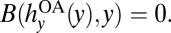Total rent dissipation is a strong assumption for a recreational fishery. However, this feature is adopted by the majority of bioeconomic research on open access problems and captures the essential effects that unregulated angling, relative to more efficient management, results in overharvesting and reduces the value of the fishery (10, 29). These effects also arise in more complex models involving less-than-total rent dissipation (see, e.g., refs. 29 and 30), and so our current assumptions do not affect our qualitative result that the incentives for crayfish controls are reduced under open access. Indeed, our model is best viewed as being designed to illustrate the basic principles involved.

The agency's objective is to improve social economic welfare (SW). SW is defined as the present value of net benefits to anglers, B(h_y, y), less the costs of crayfish removal, C(h_x, x) (SI Text S2). Given SW, along with anglers’ incentives to harvest until B = 0, the agency has incentives to regulate anglers to reduce the overall harvest so that B > 0 and the fishery becomes a sustainable source of economic value (10). The agency may also have incentives to directly harvest crayfish to reduce adverse impacts crayfish have on the bass fishery.

The agency's ability to act on its incentives depends on institutional arrangements facilitating resource management, as institutions do not necessarily evolve to support maximization of SW (31). We model institutional arrangements by the set of decisions managers control, Ω. We assume h_x = 0 if the agency has no budget or authorization to remove crayfish, so that h_x ∉ Ω. When h_y ∉ Ω, the agency cannot regulate anglers and h_y = For any h_z ∈ Ω (z = x, y), the agency makes the choice to balance the associated economic and ecological trade-offs. Having both h_y and h_x in Ω is akin to having strong institutions. Failure to manage one or more species represents a degree of institutional failure. Although reality usually lies between the strong institutions and the various institutional failures we consider, these extreme cases bound the possible outcomes and illustrate the role of institutions and management behavior in shaping “ecological” thresholds and SES topology.

Assuming a discount rate of ρ, the agency's management problem is

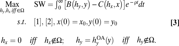The optimality conditions and solutions to problem Eq. 3 are derived in SI Text S2. The solution to problem Eq. 3 is a set of feedback response functions, h_x(x, y; Ω) and h_y(x, y; Ω), that are substituted into the dynamic system Eqs. 1 and 2. Bass harvests are h_y(x, y; Ω) = when anglers are unrestricted (h_y ∉ Ω). Crayfish harvests are h_x(x, y; Ω) = 0 when h_x ∉ Ω. When the agency can optimally manage h_x and/or h_y, the role of management is to alter the feedback responses, thereby altering the dynamic system Eqs. 1 and 2.

Results

Our bioeconomic results are presented for four scenarios (I–IV) representing four polar institutional settings based on the following combinations: unregulated versus regulated angling and agency harvests of crayfish versus no such harvests. We begin, however, with a general discussion of thresholds, which are fundamental components of our bioeconomic results.

Thresholds.

A common starting point when analyzing ecosystem management is to consider the ecological system (Eqs. 1 and 2) as if it were decoupled from the human system, such that harvest levels are not defined as feedback functions derived from a decision model. Such exercises involve setting harvest levels exogenously—chosen by the analyst and not determined within the model. Standard practice involves setting harvests at zero, fixed constant values, or fixed proportions to the stock (i.e., h_z = θ_zz, for z = x, y, where θ_z is a fixed parameter), with the fixed values being set at reasonable levels.

Fig. 3 depicts the phase plane when both control variables are set at zero. In this scenario, crayfish–bass dynamics contain one unstable equilibrium (C⁰) and two locally stable equilibria—the non-outbreak equilibrium (A⁰) and the outbreak equilibrium (B⁰). A threshold divides the state space into two basins of attraction. The system moves toward the non-outbreak basin of attraction for initial values of (x, y) to the left of the threshold and toward the outbreak basin of attraction for initial values to the right of the threshold (Fig. 3).

Fig. 3.

Multistability in the decoupled system. The dx/dt = 0 and dy/dt = 0 curves are the nullclines for the decoupled system, with points A⁰, B⁰, and C⁰ representing the equilibrium points. Points A⁰ (non-outbreak) and B⁰ (outbreak) are locally stable, whereas C⁰ is unstable. The dashed line, y^T(x; θ_x, θ_y) is the threshold between basins of attraction. Arrows represent sample trajectories.

Formally, the threshold for the decoupled system, defined as y^T(x; θ_x, θ_y) for fixed proportional harvests, solves

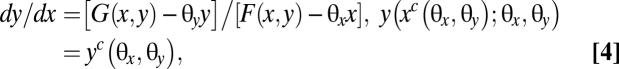where the point (x^c(θ_x, θ_y), y^c(θ_x, θ_y)) defines the unstable equilibrium C⁰, given the fixed harvest rates θ_x and θ_y. An increase in the fixed value θ_y shifts the y nullcline to increase the outbreak basin of attraction. An increase in the fixed value θ_x shifts the x nullcline to decrease the outbreak basin of attraction. Moderate, exogenously chosen, harvest rates result in qualitatively similar phase dynamics. However, a single basin may emerge for a sufficiently large fixed value of either harvest rate.

The decoupled system in Fig. 3 (or variations of it) is not an unmanaged SES, but rather a highly controlled system where the manager chooses to completely exclude all SES interactions; the system is decoupled by an implicit institution. We illustrate in our discussion of SES scenario I that incorrectly treating the decoupled system as the unmanaged system can lead to ineffective management recommendations. Our bioeconomic scenarios also show that decoupling the system is unlikely to be an optimal choice by rational managers. Even if institutions exist that provide the necessary rights for decoupling (i.e., Ω = {h_x, h_y}), the decoupled analysis ignores the role of human decision making and the associated feedback responses to ecological changes. The decoupled approach of choosing fixed harvest levels (or rates) is unlikely to solve the agency's problem (Eq. 3).

The stability landscape is fundamentally different in a generalized SES. In particular, the SES threshold is determined by substituting the feedback responses h_x(x, y, Ω) and h_y(x, y, Ω) into relations Eqs.1 and 2. Then, assuming the unstable equilibrium C exists under institutional setting Ω at the value, (x^c2(Ω), y^c2(Ω)), the SES threshold solves

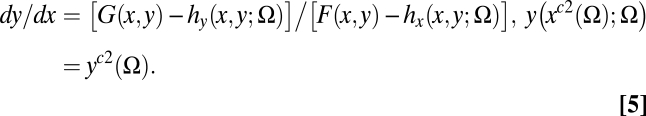The solution to Eq. 5 generally differs from the solution to Eq.4, although Eq. 4 is a special case of Eq. 5. In Eq. 5 the threshold depends on angler and agency choices within the coupled system, as well as the institutions that condition these choices. The topology of the coupled system is altered by changing the regulatory or institutional environment that determines the human responses. We now examine management under different institutional settings.

SES Scenario I: Unmanaged System (Ω = { }).

Managers in this scenario lack the ability to regulate anglers or harvest crayfish. The dynamics of this unmanaged system are governed by Eqs. 1 and 2, given the feedbacks h_y(x, y; Ω) = and h_x(x, y; Ω) = 0 (Fig. 4). A globally stable equilibrium exists in a single basin of attraction: There is no threshold. This result arises because anglers in this institutional setting lack incentives to consider the future ecological impacts of their choices and therefore do not coordinate to achieve the non-outbreak equilibrium. Moreover, because of excessive harvesting under open access angling, this unmanaged equilibrium exhibits fewer bass and more crayfish than the outbreak equilibrium in the decoupled model (Fig. 3) or in any of the scenarios we analyze below.

Fig. 4.

The unmanaged system. Starting from any initial point, the system moves to a globally stable outbreak equilibrium, A. There is no threshold.

The unmanaged system in Fig. 4, not the decoupled model of Fig. 3, is the appropriate baseline for comparing the effects of management in scenarios II–IV because it explicitly accounts for the effects of institutional arrangements on the coupled system's topology. If managers assume anglers harvest at a constant level (or rate) and that the topology of the unmanaged system is qualitatively equivalent to the decoupled model of Fig. 3, then a one-time crayfish harvest would seem adequate to move the system beyond the threshold and into the non-outbreak basin of attraction. Once in the non-outbreak basin, Fig. 3 predicts the system progresses to A without further intervention. In contrast, the phase dynamics of the true unmanaged system in Fig. 4 indicate that a one-time crayfish harvest, suggested by the decoupled model (Fig. 3), will fail because there is no alternative equilibrium. The open access institution precludes a non-outbreak equilibrium because angler behavioral responses in this setting maintain the bass population at a level required for rent dissipation, and this level is insufficient to control crayfish.

SES Scenario II: Managing Crayfish but Not Bass (Ω = {h_x}).

Optimal management in this setting is to not harvest crayfish. This is because open access bass angling prevails, so economic benefits to anglers dissipate and bass stocks are overdepleted—even in the absence of crayfish predation. With no benefits accruing in the fishery, there are no incentives to invest in protection from crayfish; it is not rational to protect the bass fishery from crayfish when we are unwilling or unable to protect the fishery from people. The solution is the same as the unmanaged outcome in scenario I and Fig. 4.

SES Scenario III: Managing Bass but Not Crayfish (Ω = {h_y}).

The bioeconomic solution involves two locally stable equilibria (A^y and B^y), with the basins of attraction separated by a Skiba threshold (15) (Fig. 5). The optimal equilibrium to pursue depends on the initial conditions (x(0), y(0)) in relation to the threshold. The dynamics for various initial conditions are indicated by the sample trajectories (Fig. 5). For instance, when the system is initially to the left of the threshold curve such as at point z, the agency optimally applies bass regulations to move the system as quickly as possible to path a^y. This path then leads to equilibrium A^y. When the system is initially to the right of the threshold curve such as at point z′, the agency optimally applies bass regulations to move the system as quickly as possible to path b^y. This path then leads to equilibrium B^y.

Fig. 5.

Managing bass but not crayfish. This feedback control diagram represents optimal bass harvest levels for different combinations of x and y (given h_x = 0). There are two locally stable equilibria, A^y (non-outbreak) and B^y (outbreak). The “Skiba threshold” divides the state space into two basins of attraction. Along the curves a^y and b^y (including the endpoint equilibria A^y and B^y), bass harvests are applied at their singular values (SI Text S2). Above these curves, bass harvests are applied at their maximum value. Below these curves, bass harvests are zero. Arrows represent sample trajectories. Trajectories for initial points to the left of the threshold, such as point z, move to path a^y and then to equilibrium A^y. Trajectories for initial points to the right of the threshold, such as point z′, move to path b^y and then to equilibrium B^y.

This bioeconomic threshold reflects human–ecological interactions given the institutional setting. The Skiba threshold differs, both in shape and in location, from the threshold in the decoupled system. This institutional setting restricts angler harvests, preventing rent dissipation and increasing the value of the bass fishery and bass conservation. However, the value of bass conservation depends on the crayfish population in relation to bass. If x is too large relative to y, significant conservation of bass is not optimal. This is because crayfish compete with humans for bass. Humans could try conserving bass, but if x is relatively large, crayfish will “free ride,” eating much of what humans conserve. This outcome leaves few incentives to conserve bass: It is not rational to control anglers if we are not willing (or able) to control crayfish predation on bass. The result is akin to an open access problem in which the unmanaged nuisance predator leads to collapse of the system.

If y is large relative to x, then crayfish are less of a concern and a degree of bass conservation is optimal. In this case bass conservation helps control the crayfish population. In effect, bass conservation leads to indirect management of crayfish. It would be more cost effective to manage crayfish directly, in which case bass harvests could be increased. However, absent an institution enabling crayfish management, extra conservation is optimal. This institutional failure leads to a larger equilibrium bass population than in any of the other scenarios we examine here, but at additional cost to society.

SES Scenario IV: Managing Both Bass and Crayfish (Ω = {h_x, h_y}).

The bioeconomic solution is a globally stable non-outbreak equilibrium in a single basin of attraction (Fig. 6). The long-run solution involves the application of continuous crayfish and bass controls that differ from a one-shot crayfish control effort suggested by the decoupled scenario (Fig. 3).

Fig. 6.

Managing crayfish and bass. This feedback control diagram represents optimal crayfish and bass harvest levels for different combinations of x and y. There is a globally stable non-outbreak equilibrium, A*, at which point both harvest levels are set at their singular values (SI Text S2). Along the curve a*, which leads to equilibrium A*, bass harvests are applied at singular values and crayfish harvests are zero. Along the curve b*, which leads to equilibrium A*, crayfish harvests are applied at singular values and bass harvests are zero. In other regions of the graph, crayfish and bass harvests are indicated by the notation {h_x, h_y}. The curves and divide the state space into regions where different values of the harvest controls are applied. Arrows represent sample trajectories.

The global optimality that exists in this scenario (Fig. 6) means there is no threshold. The institutional setting increases the value of the bass fishery by restricting angler and crayfish predation on bass, with the latter accomplished by reducing the crayfish population. The greater value of the bass fishery in this scenario always makes it optimal for the agency to prevent an outbreak. Practically speaking, the agency eliminates the threshold by targeting harvest strategies toward both species in a way that effectively targets the ecological interactions that generate multistability in the decoupled system.

The desirability of managing both species to cost effectively attain the non-outbreak state depends on costs and benefits. If, for example, the costs of removing crayfish were astronomical, we might expect the same outcome as when bass management but not crayfish management is possible (Fig. 5): Managers could target both species, but due to costs they would choose not to. Benefits also matter. In scenario IV (Fig. 6), the agency's ability to manage anglers generates sufficient benefits to incentivize crayfish removal.

Institutional Change.

Although we have not modeled institutional change as an endogenous response to resource scarcity (which is beyond the scope of the present analysis) (but see, e.g., refs. 17 and 31), our results indicate that management history will affect the desirability of implementing costly institutional changes for multistable systems. For instance, the gains from expanding the agency's rights, e.g., switching from scenario III to scenario IV, depend on whether the system is currently in the outbreak basin or the non-outbreak basin in scenario III. If the system is currently in the outbreak basin of scenario III (i.e., equilibrium B^y), then switching to scenario IV significantly improves bass conservation and may yield benefits that outweigh the costs of this institutional change. If the system is currently in the non-outbreak basin of scenario III (i.e., equilibrium A^y), then switching to scenario IV may have only a small effect on bass conservation and the benefits may not justify the costs of this institutional change.

Discussion

Our analysis shows how thresholds and multiple equilibria of multivariate ecological systems change in response to different institutions. Under strong institutions, the SES may be managed to be fairly robust to shocks so that tipping points are of little importance. This robustness declines and the role of tipping points increases, however, for weaker institutions that reduce managerial flexibility. These insights emphasize that institutions defining the rights and capacities of resource managers profoundly affect their ability to manage an SES and hence alter the bioeconomic trade-offs that guide their management decisions. This is an important extension of the notion that institutional failure is the root cause of many environmental problems (31, 32). Failure to account for, and manage, feedbacks within SESs can lead to undesirable states of the world. In contrast, appropriately accounting for such feedbacks creates the possibility for desirable states of the world and in some cases can cause undesirable states to cease to exist as possibilities. This outcome arises because coupling of the human and the ecological system allows management to act directly on the nonlinear relationships that create thresholds between alternative regimes.

We focused our numerical example on interactions between a recreationally valued fish and an invasive crayfish because fish are exploited and managed globally, and invasive crayfish are a global concern (33, 34). IGP interactions like those modeled here are common (e.g., ref. 35), and so even specific components of our model likely apply to many ecosystems of importance to humans (e.g., refs. 36 and 37). Even where other ecological interactions influence multistability, the general lesson that human behaviors, and the institutions governing them, can substantially alter stability landscapes broadly applies. Indeed, the insights may be enhanced for systems involving more ecological interactions [e.g., age structure (ref. 23) or more species] that are capable of being managed, as the role of institutions grows in such settings. The insights may also be relevant for other types of SESs, as regime shifts and multistability may arise in a SES even if the decoupled ecological system does not exhibit multistability (16, 38) (see SI Text S2 for a sensitivity analysis of our model results). Quantified threshold values that ignore institutions provide little guidance for policymakers. The key is to identify the structural ecological and socioeconomic relationships that lead to multistabiltiy within the SES, so that institutions may be developed to target these SES relationships.

References

- 1.Scheffer M, Carpenter S. Catastrophic regime shifts in ecosystems: Linking theory to observation. Trends Ecol Evol. 2003;18:648–656. [Google Scholar]
- 2.Schröder A, Persson L, De Roos AM. Direct experimental evidence for alternative stable states: A review. Oikos. 2005;110:3–19. [Google Scholar]
- 3.Beisner BE, Haydon DT, Cuddington K. Alternative stable states in ecology. Front Ecol Environ. 2003;1:376–382. [Google Scholar]
- 4.Lenton TM, et al. Tipping elements in the Earth's climate system. Proc Natl Acad Sci USA. 2008;105:1786–1793. doi: 10.1073/pnas.0705414105. [DOI] [PMC free article] [PubMed] [Google Scholar]
- 5.Rockström J, et al. A safe operating space for humanity. Nature. 2009;461:472–475. doi: 10.1038/461472a. [DOI] [PubMed] [Google Scholar]
- 6.Schellnhuber HJ. Tipping elements in the Earth system. Proc Natl Acad Sci USA. 2009;106:20561–20563. doi: 10.1073/pnas.0911106106. [DOI] [PMC free article] [PubMed] [Google Scholar]
- 7.Carpenter SR, Bennett EA, Peterson GD. Scenarios for ecosystem services: An overview. Ecol Soc. 2006;11:29. [Google Scholar]
- 8.Walker B, Holling CS, Carpenter SR, Kinzig A. Resilience, adaptability, and transformability in social-ecological systems. Ecol Soc. 2004;9:5. [Google Scholar]
- 9.Perrings C, Walker B. Biodiversity, resilience and the control of ecological-economic systems: The case of fire-driven rangelands. Ecol Econ. 1997;22:73–83. [Google Scholar]
- 10.Clark CW. Mathematical Bioeconomics Optimal Management of Renewable Resources. 2nd Ed. Hoboken, NJ: Wiley; 2005. [Google Scholar]
- 11.Janssen MA, Anderies JM, Walker BH. Robust strategies for managing rangelands with multiple stable attractors. J Environ Econ Manage. 2004;47:140–162. [Google Scholar]
- 12.Crepin A. Using fast and slow processes to manage resources with thresholds. Environ Resour Econ. 2007;36:191–213. [Google Scholar]
- 13.Biggs R, Carpenter SR, Brock WA. Turning back from the brink: Detecting an impending regime shift in time to avert it. Proc Natl Acad Sci USA. 2009;106:826–831. doi: 10.1073/pnas.0811729106. [DOI] [PMC free article] [PubMed] [Google Scholar]
- 14.Carpenter SA, Ludwig D, Brock WA. Management of eutrophication for lakes subject to potentially irreversible change. Ecol Appl. 1999;9:751–771. [Google Scholar]
- 15.Mäler K-G, Xepapadeas A, de Zeeuw A. The economics of shallow lakes. Environ Resour Econ. 2003;26:603–624. [Google Scholar]
- 16.Dasgupta P, Maler K-G. The economics of non-convex ecosystems: introduction. Environ Resour Econ. 2003;26:499–525. [Google Scholar]
- 17.North DC. Institutions, Institutional Change and Economic Performance. New York: Cambridge Univ Press; 1990. [Google Scholar]
- 18.Brock WA, Carpenter SR. Panaceas and diversification of environmental policy. Proc Natl Acad Sci USA. 2007;104:15206–15211. doi: 10.1073/pnas.0702096104. [DOI] [PMC free article] [PubMed] [Google Scholar]
- 19.Suding KN, Hobbs RJ. Threshold models in restoration and conservation: A developing framework. Trends Ecol Evol. 2009;24:271–279. doi: 10.1016/j.tree.2008.11.012. [DOI] [PubMed] [Google Scholar]
- 20.Arrow K, et al. Managing ecosystem resources. Environ Sci Technol. 2000;34:1401–1406. [Google Scholar]
- 21.Groffman PM, et al. Ecological thresholds: The key to successful environmental management or an important concept with no practical application? Ecosystems (N Y) 2006;9:1–13. [Google Scholar]
- 22.Dorn NJ, Mittelbach GG. More than predator and prey: A review of interactions between fish and crayfish. Vie Milieu. 1999;49:229–237. [Google Scholar]
- 23.Polis GA, Meyers CA, Holt RD. The ecology and evolution of intraguild predation: Potential competitors that eat each other. Annu Rev Ecol Syst. 1989;20:297–330. [Google Scholar]
- 24.Mayer AL, Rietkerk M. The dynamic regime concept for ecosystem management and restoration. Bioscience. 2004;54:1013–1020. [Google Scholar]
- 25.Sharp BR, Whittaker RJ. The irreversible cattle-driven transformation of a seasonally flooded Australian savanna. J Biogeogr. 2003;30:783–802. [Google Scholar]
- 26.Jackson JBC, et al. Historical overfishing and the recent collapse of coastal ecosystems. Science. 2001;293:629–637. doi: 10.1126/science.1059199. [DOI] [PubMed] [Google Scholar]
- 27.Mylius SD, Klumpers K, de Roos AM, Persson L. Impact of intraguild predation and stage structure on simple communities along a productivity gradient. Am Nat. 2001;158:259–276. doi: 10.1086/321321. [DOI] [PubMed] [Google Scholar]
- 28.Drury KLS, Lodge DM. Using mean first passage times to quantify equilibrium resilience in perturbed intraguild predation systems. Theor Ecol. 2009;2:41–51. [Google Scholar]
- 29.Anderson LG. Toward a complete economic theory of the utilization and management of recreational fisheries. J Environ Econ Manage. 1993;24:272–295. [Google Scholar]
- 30.Abbott JK, Wilen JE. Rent dissipation and efficient rationalization in for-hire recreational fishing. J Environ Econ Manage. 2009;58:300–314. [Google Scholar]
- 31.Ostrom E. Governing the Commons: The Evolution of Institutions for Collective Action. Cambridge, UK: Cambridge Univ Press; 1990. [Google Scholar]
- 32.Dietz T, Ostrom E, Stern PC. The struggle to govern the commons. Science. 2003;302:1907–1912. doi: 10.1126/science.1091015. [DOI] [PubMed] [Google Scholar]
- 33.Peters JA, Lodge DM. Invasive species policy at the regional level: A multiple weak links problem. Fisheries (Bethesda, Md) 2009;34:373–381. [Google Scholar]
- 34.Lodge DM, Taylor CA, Holdich DM, Skurdal J. Nonindigenous crayfishes threaten North American freshwater biodiversity: Lessons from Europe. Fisheries (Bethesda, Md) 2000;25:7–20. [Google Scholar]
- 35.Daskalov GM, Grishin AN, Rodionov S, Mihneva V. Trophic cascades triggered by overfishing reveal possible mechanisms of ecosystem regime shifts. Proc Natl Acad Sci USA. 2007;104:10518–10523. doi: 10.1073/pnas.0701100104. [DOI] [PMC free article] [PubMed] [Google Scholar]
- 36.Daskalov GM, Mamedov EV. Integrated fisheries assessment and possible causes for the collapse of anchovy kilka in the Caspian Sea. ICES J Mar Sci. 2006;64:503–511. [Google Scholar]
- 37.Gutman M, Henkin Z, Holzer Z, Noy-Meir I, Sligman NG. A case study of beef-cattle grazing in a Mediterranean-type woodland. Agrofor Syst. 2000;48:119–140. [Google Scholar]
- 38.Brander JA, Taylor MS. The simple economics of Easter Island: A Ricardo-Malthus model of renewable resource use. Am Econ Rev. 1998;88:110–138. [Google Scholar]
Associated Data
This section collects any data citations, data availability statements, or supplementary materials included in this article.