Forming classes by stimulus frequency: Behavior and theory

Abstract

Visual classification is the way we relate to different images in our environment as if they were the same, while relating differently to other collections of stimuli (e.g., human vs. animal faces). It is still not clear, however, how the brain forms such classes, especially when introduced with new or changing environments. To isolate a perception-based mechanism underlying class representation, we studied unsupervised classification of an incoming stream of simple images. Classification patterns were clearly affected by stimulus frequency distribution, although subjects were unaware of this distribution. There was a common bias to locate class centers near the most frequent stimuli and their boundaries near the least frequent stimuli. Responses were also faster for more frequent stimuli. Using a minimal, biologically based neural-network model, we demonstrate that a simple, self-organizing representation mechanism based on overlapping tuning curves and slow Hebbian learning suffices to ensure classification. Combined behavioral and theoretical results predict large tuning overlap, implicating posterior infero-temporal cortex as a possible site of classification.

There is a natural tendency to relate perceived exemplars to particular classes (1, 2). However, despite evidence suggesting a perceptual basis for the representation of visual classes (3–6), we still do not know how these are formed in the brain. Can class representations evolve autonomously by our exposure to the environment (7, 8) or do we need feedback or an external teacher labeling information or context?

Classes formed by self-organizing mechanisms are likely to reflect environmental structure (7–10). For example, co-occurring discontinuities along correlated features of real-world attributes may become locations of category boundaries (1). Repeated environmental experience also mediates development of perception-based expertise (11, 12). For example, although young children are about as good at recognizing upright and inverted faces, adults are much better at recognizing upright faces (11). Development of expertise seems to be accompanied by modified internal (face) representation, whereby more frequent features (upright faces) are more closely associated with image class.

Perceptual classification studies traditionally involve supervised tasks (13–19) or instructions regarding the classes (20). However, supervision dictates class structure and precludes isolation of self-organizing mechanisms. A few studies dealt with unsupervised classification, with stimuli constructed from several prototypes (21, 22). In accord with a self-organizing representation mechanism, there was significant overlap in class membership with stimulation structure, but because analysis focused only on the overlap and not on classification pattern, not much could be concluded about underlying representation mechanisms. Other studies touched indirectly on unsupervised classification, e.g., when dealing with encoding attribute frequency (23) or correlations (24), incidental learning (25), or perceptual development (26).

Some theorists proposed a self-organizing representation mechanism based on a priori expectations about stimulus distribution, which is adjusted by incoming stimulation (17, 27). Others assumed that following exposure to a new environment a one-shot abstraction is stored, with details of further exposures compared with this abstraction (8). Updating might be dictated by the frequency of attribute values (9) or their associations (1, 24). All of these suggestions assumed that self-organization is based on a nonuniform distribution of features across stimuli.

The present study was designed to isolate experimentally a self-organizing representation mechanism underlying class formation and to analyze its characteristics. Our working hypothesis was that such a mechanism would be affected by the statistics of stimulation. We study unsupervised classification of stimuli that vary only along one physical dimension and find that classification correlates with stimulation statistics and that this correlation evolves autonomously. Using a minimal, biologically based, neural-network simulation, we demonstrate that a self-organizing mechanism suffices to explain our findings.

Behavioral Testing

Methods.

Fifty-seven adult subjects with normal or corrected-to-normal vision sorted stimuli into classes without prior demonstration or instruction concerning the structure or number of classes and without performance feedback (Fig. 1A). Instructions on the computer monitor informed subjects only that they would see stimuli of one or more kinds and should classify them accordingly. Eight keys on the computer keyboard were available for responses.

Figure 1.

Classification task. (A) Subjects classified stimuli one by one without feedback or prior information regarding class structure. A blank gray screen preceded each trial, initiated by key-press. After 1 s, a small fixation cross appeared, followed (200 ms later) by a stimulus. At 500 ms after stimulus onset, the screen was blanked again. Subjects had 1.5 s from stimulus onset to relate it to a class. Late responses were discarded and signaled to the subjects. (B) Examples of stimuli used for classification. (C) Statistical distributions of the stimuli, reflecting the frequency of their presentation. Each subject participated in one of the three possible distribution conditions during all of the sessions.

Stimuli consisted of a pair of identical vertical bright stripes presented 115 cm away on a gray screen (1,280 × 1,024 pixels; 36 pixels/cm; 21-inch SGI Indy; Fig. 1B). Stripe height was the full screen, and stripe centers were 256 pixels from central fixation. Serially presented stimuli varied only by the width of the stripes (1–512 pixels, divided into 36 sampling bins). Each classification session included 1,024 trials.

Three subject groups differed only by the distribution of the stimuli presented to them (during all of the sessions; Fig. 1C). Two distributions had three or four Gaussian peaks, respectively, with interpeak intervals six times the Gaussian σ. For the third distribution, stimuli were sampled uniformly. Data of 16, 8, and 10 subjects were used in statistical analysis of the three- and four-peaked and uniform distribution cases, after excluding classifiers with extremely broad classes (>16 stimulus bins in the last two sessions; e.g., Fig. 2, subject KR).

Figure 2.

Cross-subject classification strategy variability. Individual examples of classification strategies of three subjects during their fourth session classifying stimuli sampled from the three-peak distribution. Graphs present sorting coherence for each stimulus (fraction of presentations in a bin attributed to a class; each symbol represents a particular class). Gray curves plot, here and below, the relative presentation frequency in the session. Similar strategies were found for the four-peak and uniform cases. The stimulus range here and below is in bins.

A single observation session of 256 trials preceded the main classification sessions, acquainting subjects with task procedure and stimulus distribution. Here subjects pressed the same key for all stimuli.

Results.

Classification strategies varied largely among subjects, as reflected in the individual examples (Fig. 2) and large variability in number of classes (SD > 2 classes, in all cases for fourth session) and broadest class width (SD > 13% of whole range).

Despite this variability, a closer view reveals basic perceptual factors in class formation: Fig. 3A presents location histograms of class centers and class boundaries during the fourth session of each subject group. In the multipeak cases, subjects were most likely to locate class centers near the most frequent stimuli (i.e., near the peaks of the stimulus distributions). At the same time, class boundaries were most likely to be located near the least frequent stimuli (i.e., the distribution minima). In the uniform-distribution case, no clear pattern is seen. Classification dependence on stimulus distribution is highly significant, as demonstrated in Table 1.

Figure 3.

Stimulus distribution effect on classification. (A) Histograms of class center (Left) and boundary (Right) location for each case, during the fourth classification session, reflecting clear correlation with the statistical pattern of the stimulation in the multipeak cases. Bars of each histogram denote percentage of subjects who had a class center (boundary) at each stimulus. Class center location was computed as the center of gravity of the sorting coherence function, χ, between the two boundaries, i.e., Σb ⋅ χ(b, c)/Σχ(b, c). Dashed lines indicate range of edge effects. (B) Cross-session development of the distribution effect: the center and boundary location histograms of each session are reorganized according to distance from the nearest peak. Bars indicate average percent of subjects locating center or boundary at a specific distance from distribution peak. Error bars denote SD. Numbers are correlations between histograms and the distribution characteristics. Note slower evolution of the effects in the four-peak case. (C) Distribution effect on decision speed. Colored curves indicate cross-subject average behavioral RT data (Left) and simulation convergence time τ (Right). Error bars denote SE and SD of the behavioral and simulation results, respectively. The longer RTs near less frequent stimuli was successfully imitated by the simulation τ. However, τ increased near range edges, where RTs were shorter. (D) Absence of subject awareness of the statistical structure of the stimuli. Dark curves present the cross-subject average subjective rate of presentation frequency (on a five-level scale; normalized between lowest and highest). Data were collected after completion of the classification experiment, where subjects were asked to estimate the frequency of a few serially presented stimuli (usually 15; always including the most and least frequent). Symbols indicate individual estimates. Subjective estimations were not correlated with actual stimulus distributions.

Table 1.

Correlation between stimulus distributions and class structure (session 4)

Stimulus distribution	Subject group
	3-peak	4-peak	Uniform
Correlation with class centers
3 peaks	0.80	−0.03	−0.01
4 peaks	−0.22	0.81	0.43
Correlation with class boundaries
3 peaks	0.72	−0.36	−0.21
4 peaks	−0.27	0.59	−0.11

Bins related to edge effect were ignored. For the boundary location histogram, the Pearson correlation was computed with stimulation infrequency: bins with likelihood <6/session were set to 1; all others to 0. 

The cross-session evolution of the distribution effects is different in the two multipeak cases (Fig. 3B). With three peaks, a strong effect on center location was apparent already in the first session, whereas with four peaks it evolved only in the second. The effect on boundary location appeared later for both distributions, but still with the effect for four peaks lagging behind that with three peaks.

Center and boundary location histograms also show an edge effect, suggesting special sensitivity to stimuli near the edges. In the three-peak case, there are two clear additional humps in the center-location histogram near the edges of the stimulus range (Fig. 3A, dashed lines). A similar edge effect exists in the uniform and four-peak cases, where the effect is less noticeable because of the proximity of the extreme stimulus-distribution peaks to the stimulus range edges.

Subject response time (RT) was also affected by stimulus statistics (Fig. 3C Left). In the three-peak case, there is a clear tendency for longer RT near the two middle distribution minima. This pattern appears also in the four-peak case, where it is slower to develop; intriguingly, the cross-stimulus average RT is longer than with three peaks. An opposite, RT diminution effect is seen for stimuli near the edges (except with three peaks for the most narrow stripes) despite the low frequency here in the multipeak cases. The absence of augmentation near the edges, even when they are rarely sampled, eliminates the possibility that augmentation at the middle minima results from the relative novelty of these stimuli. Instead, it seems to reflect distribution effects on boundary location.

Surprisingly, despite long testing periods (4,000–10,000 presentations) and the stimulus distribution effect on class pattern and RT, subjects were not aware of the presentation distribution. Fig. 3D demonstrates subject subjective evaluation of stimulus frequency (following completion of the classification sessions), compared with the actual presentation likelihood of the stimuli. No correspondence is seen to the details of the distributions (in contrast to claims of subject awareness of stimulus frequency in other cases; ref. 28). Furthermore, no individual subject showed such awareness. This suggests that mechanisms underlying the distribution effect act automatically. We found another edge effect here—a tendency to think that edge stimuli were rare, even when they were sampled frequently (in the uniform case).

Modeling and Simulation

The implicit and direct distribution effects suggest a simple self-organizing underlying mechanism. To test this hypothesis, we designed a simulation network composed of excitatory and inhibitory neurons. The fully interconnected excitatory neurons (n = 500) are described as a unidimensional array, reflecting only the assumption that similar stimuli activate overlapping neuron groups—similar to a typical cortical feature map of the variable dimension but without synaptic dependence on distance (see ref. 29 for a classical, feed-forward categorization model). Each stimulus S_i (i = 1 . . . 500) excites consecutive neurons forming a fraction f = 1/3 of the network. (nf = 167; i − nf/2 to i + nf/2; fewer if i is near an edge). With such a network configuration, f corresponds to the initial neuronal tuning width and the center of the evoking range may be called the neuron's “preferred stimulus.” (Although biological tuning may be more Gaussian-like, a square wave is simpler and leads to the same qualitative results.) Equations for network dynamics are described in the Appendix. External input leads to recurrent excitation and inhibition that converges to a steady state, with inhibitory neuron activity counterbalancing global self-excitation.

Synaptic efficacies have two stable states (see Appendix). The simulation starts with an arbitrary, low fraction of synapses in the potentiated state. Following each stimulus, the excitatory-to-excitatory synaptic coupling strengths are updated (neglecting recurrent activity effects) according to stochastic Hebbian rules: long-term synaptic potentiation is triggered by simultaneous elevated activity in pre- and postsynaptic neurons, while an activity mismatch induces long-term depression. Learning must be slow enough so that the memory span (limited by the number of stable synaptic efficacies; refs. 30 and 31) includes a sufficient number of stimulus presentations to reasonably sample the distribution and allow it to be reflected in the synaptic matrix.

Synaptic Dynamics.

The development of the synaptic matrices (of the excitatory network) for each stimulus distribution is presented in Fig. 4A. In all cases, we observe potentiation of connections along the diagonal (i ≈ j for neighboring neurons) falling off with distance (as probability for coactivation decreases and probability for activation of one but not the other increases).

Figure 4.

Simulation results for each distribution case. (A) The synaptic matrix—color-coded density of potentiated synapses from neuron j to neuron i—across “sessions,” reflecting changes in the synaptic configuration during learning. Different matrices columns correspond to different sampling distribution. Each synaptic matrix is plotted at four stages of simulation. Connectivity patterns evolve gradually. The diagonal pattern reflects the high potentiation probability between neighboring neurons. In the multipeak cases potentiated connections are clustered in clouds that correspond to the distribution peaks both in number and scope. Note slower evolution for four peaks than for three peaks, resulting from simulation with a large overlap between neurons. (B) Activity map across “sessions” (rows) and stimulus distributions (columns). Each map reflects the activity level (color-coded) of each neuron (y axis) as a function of the stimuli (x axis; activity is averaged across 20 simulation runs at the 1,000th iteration, i.e., near activity asymptote). The simulation of each activity map was run using its corresponding synaptic matrix (A). After 500 stimulus presentations, there is only weak activity along the diagonal reflecting original stimulus-evoked excitation. In the multipeak cases, further stimulation leads to clustered activity that is correlated with the statistical structure of the stimulation, while in the uniform case unstructured activity is seen. Note the delayed evolution of clustered activity in the four-peak case relative to the three-peak case.

For peaked distributions, clouds of potentiated connections evolve corresponding to the distribution peaks. Pairs of neurons with preferred stimuli that straddle frequency peaks have many more common evoking stimuli —potentiating synaptic interconnections—and fewer unshared inputs—depressing interconnections—than do pairs straddling frequency minima. The result is a gradient in density of potentiated synapses—from those among neurons that are activated by less frequent stimuli (few stimuli coactivate such neuron pairs; many activate one or the other) toward those among neurons activated by more frequent stimuli (many coactivating stimuli; few activate only one). The final structure clearly exhibits the expected dependence on stimulus distribution. Note that this type of synaptic matrix is only formed provided that the number nf of neurons activated by each stimulus is large enough to enable the connectivity gradient, and small enough to sense differences in stimulus frequencies (see below).

Neuronal Activity.

Given this synaptic structure, network activity is attracted toward patterns that initially corresponded to the most frequent stimuli (the peaks of the distribution). Basins of attraction can be considered as internal class representations. These attractors are separated by (less consistent) activity patterns evoked by stimuli at the distribution minima, which therefore correspond to class boundaries. Fig. 4B presents average excitatory activity maps (neuronal response as a function of stimulus) following convergence into an attractor state, for each distribution, and at several stages of simulation. After 500 presentations (top row), any stimulation leads to weak network activation, and the final response just reflects the applied input current. With more presentations, more synapses are potentiated and network global activity increases forming strong reverberations. Synaptic structure is apparent in square-like clouds of elevated activity, corresponding to the number of distribution peaks—i.e., groups of similar stimuli tend to produce the same final response. Class boundaries are determined by the borders of the basins of attraction, located at the distribution minima. Near the minima the network response is inconsistent across runs with similar presentation conditions (ending up in one of the two nearest attractors). Activity patterns are formed earlier with three than with four peaks, as found in the behavioral experiment.

In the uniform case, no consistent structured pattern of activity is seen, except for weak but consistent enhanced activity near the edges. The simulation showed activity-pattern variability across learning stages (smeared by averaging) corresponding to the unstable classification patterns found behaviorally.

Evolution Rate and Tuning Width.

Interestingly, the stronger and faster behavioral distribution effect that we found behaviorally in the three-peak relative to the four-peak case imposes a lower bound on the initial neuronal tuning. When f is much broader than the distribution interpeak interval (normalized to the full range width, designated as Δμ), the connectivity gradient toward the peak becomes very weak, leading to below-optimal correlation between distribution and synaptic matrix. The shallow connectivity gradient results in a less stable activity pattern and slower learning. When f is narrow (similar to the four-peak Δμ) then the connectivity gradients with three or four peaks are similarly strong; when f is as broad as the three-peak Δμ, the gradient is already below optimal for the four-peak case (see supplemental material, which is published on the PNAS web site, www.pnas.org). Thus, the behavioral constraint implies the surprising prediction of a very broad tuning width—spanning as much as a third of the stimulus range used in the experiments. This value of f was used in the simulations leading to the results presented above.

Network “RT”.

Although we did not intend that the model explain subject decision mechanisms, the network convergence time, τ§, dependence on stimulus frequency (Fig. 3C Right) is strikingly similar to that of the behavioral RT (Fig. 3C Left). With peaked distributions, these times are longer for stimuli near distribution minima. The slow build-up of excitatory activity is attributable to both low density of potentiated synapses near the minima and competition between two neighboring attractors. In the uniform case, convergence time is similar for all stimuli (except at the edges), as in the behavioral experiment. The model does not explain faster RTs at the distribution edges.

Discussion

The behavioral experiments revealed four novel findings. Unsupervised classification of simple stimuli leads to formation of common classification and RT patterns, which highly reflect the statistical structure of the stimulation. Class boundaries tend to be located near the least frequent stimuli and classes tend to be centered near the most frequent stimuli. The quality and evolution speed of these classification patterns is also affected by stimulus distribution. Surprisingly, subjects lacked explicit knowledge of the stimulus statistical distribution, even after long testing periods.

Formation of common classification patterns in the absence of external supervision implies an internal self-organizing mechanism. The dependence of these patterns on stimulation distribution rather than on specific stimulus values eliminates innate, hard-wired stimulus representation structures, suggesting instead a mechanism that is updated by the incoming stream of stimuli. The absence of awareness of stimulus statistics implies an automatic learning mechanism. The ability of amnesic patients to learn to classify simple stimuli might be attributable to a similar mechanism (32).

Taken together, these considerations suggest that a simple self-organizing representation mechanism underlies the distribution effect on classification. We demonstrated how a simple and general biology-based model accounts for such a mechanism. Minimal assumptions concerning neuronal configuration (unstructured network of neurons with overlapping tuning) and synaptic change (stochastic Hebbian rules of potentiation and depression) are sufficient for encoding stimulus distribution in the synaptic matrix and enabling distribution-dependent attractors that imitate behavioral results. Attractor evolution does not require top-down processes. In the model simulation, attractor boundaries (i.e., regions of confusion between attractors, analogous to class boundaries) are located where synaptic depression is more probable than facilitation, i.e., the ranges of rare stimuli. Rare stimuli also require more iterations to “trap” the network activity into an attractor, supporting the conclusion that the increased RT near distribution minima (except at stimulus range edges) results from the same mechanism that underlies boundary location.

Simulation results make several predictions. Requiring the model to fit the experimental finding of faster learning with three rather than with four peaks implies very broad tuning. Single neurons are evoked by ≈1/3 of the broad stimulus range used in the experiment. This constraint suggests that the locus of processing may be human homologues of monkey posterior infero-temporal cortex, where neurons are selective to simple stimulus features but are broadly tuned (33). Indeed, partial lesions of these cortices (in monkeys) impair classification of stimuli that vary along one dimension, whereas lesions in lower-level cortices do not (34). The broad tuning constraint also suggests that a five-peak distribution (under similar experimental conditions) would be too crowded to reflect the distribution effect. Additionally, with four peaks learning should reveal attractors that are narrower than the original neuron tuning. Brain imaging techniques might reveal this tuning change.

The simulation findings also predict that introducing changes in stimulus statistical distribution following practice will lead to altered attractor patterns and class structure. Preliminary results support these predictions [Rosenthal, O. & Hochstein, S. (2000) Invest. Ophthalmol. Vis. Sci., 41, S47, no. 244). Moreover, different rates of change are expected when practice starts with a three- versus a four-peak distribution and is changed to the other.

The mechanism underlying classification may be similar to that inducing specific patterns of delay activity (35, 36) or tuning width (37). Further study is required to determine whether the same self-organizing mechanism underlies other representation processes such as feature maps (38) and associative memory (35, 36). This study was based on classification along a single stimulus dimension. In natural conditions, stimuli usually vary across many attributes, raising many questions regarding their interactions in classification (18, 24).

Abbreviation

RT

response time

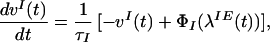
Simulation of Network Dynamics

Network dynamics are governed by the following equations (see also refs. 30, 31, 39–41):

1

2

where v^I and v are the mean inhibitory activity and mean activity of the ith excitatory neuron, respectively; τ_E and τ_I are excitatory/inhibitory neuron time constants; and Φ_E and Φ_I are excitatory/inhibitory neuron transfer functions giving the change in mean output activity as a function of total input current, λ. Φ_E(λ) = , while Φ_I(λ) = C_Iλ for λ > T_I (where T_I = 50; C_I = 0.6 are the inhibition threshold/gain) and Φ_I(λ) = 0, otherwise. λ simulates the external current in excitatory neuron i due to visual stimulation S_i and a Gaussian noise (average = 20 for stimulated neurons, 0 for others; SD = 50 for time step dt = 0.1τ_E = 0.1τ_I). Inhibitory neurons participate only in local dynamics and are described by a single mean activity variable.

Recurrent excitation/inhibition are induced by excitatory-activity-originated input currents, λ(t), and λ^IE(t) injected into excitatory/inhibitory neurons, respectively; and inhibitory-activity-originated currents, λ(t), injected into excitatory neurons. For simplicity we assume that inhibitory neurons do not receive inhibitory currents. These currents are described generally as

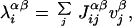where α = E, I denotes the target neuronal population, β = E, I the current generator population, and J_ij are the synaptic efficacies. Connections to/from inhibitory neurons are described by uniform synaptic efficacies (J^IE = 1.0, J^EI = 0.25).

Each excitatory synapse is assumed to have two stable states (J = 0, depressed; J = 0.25, potentiated) on time scales much longer than the time between presentations (see ref. 30). Simultaneous activation of pre- and postsynaptic neurons induces long-term synaptic potentiation with probability q₊ = 0.004. Activation of only one neuron in the pair induces long-term depression with probability q₋ = 0.002. Each presentation leaves a small trace in the synaptic matrix, as a result of a local random selection of which candidate synapses are indeed to be changed. Because the synaptic efficacies have a limited number of stable states, the network shows the palimpsest property: new presentations overwrite old ones and only part of the past is preserved.

Because q₊ and q₋ are small, the probability that the synapse between neurons i and j is eventually in the potentiated state is (see ref. 31):

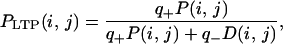where P(i, j) and D(i, j) are respectively the fractions of the presentation events that tend to potentiate and depress the synapse.

References

- 1.Rosch E, Mervis C B, Gray W D, Johnson D M, Boyes-Braem P. Cognit Psychol. 1976;8:382–439. [Google Scholar]
- 2.Roberts W A. In: Advances in Psychology: Stimulus Class Formation in Humans and Animals. Zentall T R, Smeets P M, editors. Vol. 117. Amsterdam: Elsevier; 1996. pp. 35–54. [Google Scholar]
- 3.Malach R, Reppas J B, Benson R R, Kwong K K, Jiang H, Kennedy W A, Ledden P J, Brady T J, Rosen B R, Tootell R B. Proc Natl Acad Sci USA. 1995;92:8135–8139. doi: 10.1073/pnas.92.18.8135. [DOI] [PMC free article] [PubMed] [Google Scholar]
- 4.Logothetis N, Sheinberg D L. Annu Rev Neurosci. 1996;19:577–621. doi: 10.1146/annurev.ne.19.030196.003045. [DOI] [PubMed] [Google Scholar]
- 5.Tanaka K. Curr Opin Neurobiol. 1997;7:523–529. doi: 10.1016/s0959-4388(97)80032-3. [DOI] [PubMed] [Google Scholar]
- 6.Kourtzi Z, Kanwisher N. J Neurosci. 2000;20:3310–3318. doi: 10.1523/JNEUROSCI.20-09-03310.2000. [DOI] [PMC free article] [PubMed] [Google Scholar]
- 7.Gibson J J, Gibson E J. Psychol Rev. 1955;62:32–41. doi: 10.1037/h0048826. [DOI] [PubMed] [Google Scholar]
- 8.Evans S H. Psychol Sci. 1967;8:87–88. [Google Scholar]
- 9.Rumelhart E, Zipser D. Cognit Sci. 1985;9:75–112. [Google Scholar]
- 10.Kohonen T. Self Organizing Maps. Berlin: Springer; 1995. [Google Scholar]
- 11.Carey S, Diamond R. Science. 1977;195:312–314. doi: 10.1126/science.831281. [DOI] [PubMed] [Google Scholar]
- 12.Gauthier I, Tarr M J. Vis Res. 1997;37:1673–1682. doi: 10.1016/s0042-6989(96)00286-6. [DOI] [PubMed] [Google Scholar]
- 13.Shepard R N, Hovland C I, Jenkins H M. Psychol Monogr. 1961;75:1–42. [Google Scholar]
- 14.Posner M I, Keele S W. J Exp Psychol. 1968;77:353–363. doi: 10.1037/h0025953. [DOI] [PubMed] [Google Scholar]
- 15.Reed S K. Cognition: Theory and Applications. Belmont, CA: Wadsworth; 1972. [Google Scholar]
- 16.Medin D L, Schaffer M M. Psychol Rev. 1978;85:207–238. [Google Scholar]
- 17.Fried L S, Holyoak K J. J Exp Psychol Learn Mem Cognit. 1984;10:234–257. doi: 10.1037//0278-7393.10.2.234. [DOI] [PubMed] [Google Scholar]
- 18.Nosofsky R M. J Exp Psychol Gen. 1986;115:39–57. doi: 10.1037//0096-3445.115.1.39. [DOI] [PubMed] [Google Scholar]
- 19.Estes W K. Classification and Cognition. London: Oxford Univ. Press; 1994. [Google Scholar]
- 20.Homa D, Cultice J. J Exp Psychol Learn Mem Cognit. 1984;10:83–94. [Google Scholar]
- 21.Bersted C, Brown B R, Evans S H. Percept Psychophys. 1969;6:409–413. [Google Scholar]
- 22.Wills A J, McLaren I P L. Q J Exp Psychol B. 1998;51b:253–270. [Google Scholar]
- 23.Neumann P G. Mem Cognit. 1977;5:187–197. doi: 10.3758/BF03197361. [DOI] [PubMed] [Google Scholar]
- 24.Anderson J R, Fincham J M. J Exp Psychol Learn Mem Cognit. 1996;22:259–277. doi: 10.1037//0278-7393.22.2.259. [DOI] [PubMed] [Google Scholar]
- 25.Roberts P L, MacLeod C. Q J Exp Psychol A. 1995;48a:296–319. doi: 10.1080/14640749508401392. [DOI] [PubMed] [Google Scholar]
- 26.Younger B A. Child Dev. 1985;56:1574–1583. [PubMed] [Google Scholar]
- 27.Shepard R N. Science. 1987;237:1317–1323. doi: 10.1126/science.3629243. [DOI] [PubMed] [Google Scholar]
- 28.Hasher L, Zacks R T, Rose K C, Sanft H. Am J Psychol. 1987;100:69–91. [PubMed] [Google Scholar]
- 29.Knapp G A, Anderson J A. J Exp Psychol Learn Mem Cognit. 1984;10:616–637. [Google Scholar]
- 30.Amit D J, Fusi S. Neural Comput. 1994;6:957–982. [Google Scholar]
- 31.Brunel N, Carusi F, Fusi S. Network. 1998;9:123–152. [PubMed] [Google Scholar]
- 32.Knowlton B J, Squire L R. Science. 1993;262:1747–1749. doi: 10.1126/science.8259522. [DOI] [PubMed] [Google Scholar]
- 33.Tanaka K, Kobatake E. J Neurophysiol. 1994;71:856–867. doi: 10.1152/jn.1994.71.3.856. [DOI] [PubMed] [Google Scholar]
- 34.Wilson M, DeBauche B A. Neuropsychologia. 1981;19:29–41. doi: 10.1016/0028-3932(81)90041-5. [DOI] [PubMed] [Google Scholar]
- 35.Miyashita Y. Nature (London) 1988;335:817–820. doi: 10.1038/335817a0. [DOI] [PubMed] [Google Scholar]
- 36.Yakovlev V, Fusi S, Berman E, Zohary E. Nat Neurosci. 1998;1:310–317. doi: 10.1038/1131. [DOI] [PubMed] [Google Scholar]
- 37.Kobatake E, Wang G, Tanaka K. J Neurophysiol. 1998;80:324–330. doi: 10.1152/jn.1998.80.1.324. [DOI] [PubMed] [Google Scholar]
- 38.Buonomano D V, Merzenich M M. Annu Rev Neurosci. 1998;21:149–186. doi: 10.1146/annurev.neuro.21.1.149. [DOI] [PubMed] [Google Scholar]
- 39.Wilson H R, Cowan J D. Biophys J. 1972;12:1–24. doi: 10.1016/S0006-3495(72)86068-5. [DOI] [PMC free article] [PubMed] [Google Scholar]
- 40.Amit D, Brunel N. Network. 1995;6:359–388. [Google Scholar]
- 41.Amit D, Brunel N. Cereb Cortex. 1997;7:237–252. doi: 10.1093/cercor/7.3.237. [DOI] [PubMed] [Google Scholar]
Associated Data
This section collects any data citations, data availability statements, or supplementary materials included in this article.