Design and Analysis of Multiple Diseases Genome-wide Association Studies without Controls

Abstract

In genome-wide association studies (GWAS), multiple diseases with shared controls is one of the case-control study designs. If data obtained from these studies are appropriately analyzed, this design can have several advantages such as improving statistical power in detecting associations and reducing the time and cost in the data collection process. In this paper, we propose a study design for GWAS which involves multiple diseases but without controls. We also propose corresponding statistical data analysis strategy for GWAS with multiple diseases but no controls. Through a simulation study, we show that the statistical association test with the proposed study design is more powerful than the test with single disease sharing common controls, and it has comparable power to the overall test based on the whole dataset including the controls. We also apply the proposed method to a real GWAS dataset to illustrate the methodologies and the advantages of the proposed design. Some possible limitations of this study design and testing method and their solutions are also discussed. Our findings indicate the proposed study design and statistical analysis strategy could be more efficient than the usual case-control GWAS as well as those with shared controls.

1 Introduction

Due to the relatively small effect sizes of single-nucleotide polymorphisms (SNPs) in GWAS, usually a large sample is required to detect SNPs associated with the disease of interest. Since the data collection and genotyping in GWAS can be costly and time consuming, it is desirable to have study design and statistical analysis strategy that can reduce the sampling effort but without sacrificing the power in detecting significant associations.

GWAS with multiple diseases and shared controls has been conducted recently and it has been shown that GWAS with multiple diseases and shared controls is more efficient than the usual case-control GWAS where one group of cases and one group of controls are used (see, for example, The Wellcome Trust Case Control Consortium, 2007 (for convenience, we will cite this article as WTCCC, 2007 hereafter); The Wellcome Trust Case Control Consortium & The Australo-Anglo-American Spondylitis Consortium, 2007 (for convenience, we will cite this article as WTCCC & AAASC, 2007 hereafter); Craddock et al., 2010). Using shared controls will dramatically reduce the required sampling effort and the related cost and time for data collection.

Different statistical approaches can be used to detect the associated SNPs or copy number variants (CNVs) for data obtained from GWAS with multiple diseases and shared controls. For example, one can use the concept of expanded controls by treating all or part of the cases from other diseases as controls (WTCCC, 2007; WTCCC & AAASC, 2007; Craddock et al., 2010) and then apply those standard statistical association tests, such as Cochran-Armitage trend test (CATT) (Cochran, 1954; Armitage, 1955), Pearsons chi-square test and some robust tests (Freidlin et al., 2002; Zheng and Ng, 2008; Chen, 2011; Chen and Ng, 2012), to compare the individual interested disease and the pooled controls.

Chen et al (2012) have shown that the aforementioned statistical test procedures using shared controls can produce inflated false positives because multiple tests were conducted for the same SNP and decrease the statistical power in detecting associations when the Bonferroni correction was used. An alternative procedure to test for associations for GWAS with multiple diseases and shared control is the overall chi-square test applied to a (d + 1) × 3 contingency table, where d is the number of diseases. Specifically, for a given SNP, there are three possible genotypes and we have a (d + 1) × 3 contingency table, where the (d + 1)th disease is the control. Under the null hypothesis that a particular SNP is associated with none of the d diseases, the chi-square test statistic based on this (d + 1) × 3 contingency table has an asymptotic chi-square distribution with degrees of freedom (df) equal to 2d.

In this paper, we proposed a study design for GWAS in which multiple diseases are studied without controls. This study design is motivated by a real dataset of a GWAS with 4 diseases and shared controls, where we found that comparable power can be obtained by an overall chi-square test applied to the d × 3 contingency table when the shared controls are ignored. To study the power properties of the overall chi-square tests with and without controls, a simulation study is performed to compare the power of the overall test without controls with those tests with different numbers of controls. These simulation results show that when the number of diseases is not too small (say, greater than or equal to 4), using controls does not provide any gain in the statistical power.

2 Material and Methods

2.1 Pearson’s Chi-square Tests for Associations

Suppose that a SNP has two alleles, A and B, and three genotypes, AA, AB, and BB, then the counts of these three genotypes for the d diseases and a control group can be presented as a (d + 1) × 3 contingency table. To detect whether the genotype is associated with any disease, we can use the following Pearson’s chi-square test:

$${\chi }_{d+1}^2=\sum _{i=1}^{d+1}\sum _{j=1}^3\frac{{(n_{ij}-{\mu }_{ij}^{(d+1)})}^2}{{\mu }_{ij}^{(d+1)}},$$ (1)

where n_ij is the number of subjects with disease i (the d + 1 disease is representing the control) with genotype j, i = 1, 2, …, d, d + 1, j = 1, 2, 3, and ${\mu }_{ij}^{(d+1)}$ is the expected value of the n_ij . Under the null hypothesis that no association between the genotype and any disease, the genotypic frequencies for each disease should be the same as those of the control and the statistic in (1) has an asymptotic chi-square distribution with 2d df.

If the controls in the dataset are ignored, we will have a d × 3 contingency table with the last row being removed. The following chi-square test can be used:

$${\chi }_d^2=\sum _{i=1}^d\sum _{j=1}^3\frac{{(n_{ij}-{\mu }_{ij}^{(d)})}^2}{{\mu }_{ij}^{(d)}},$$ (2)

where ${\mu }_{ij}^{(d)}$ is the expected value of the n_ij . Similar to the statistic in (1), the statistic in (2) has an asymptotic chi-square distribution with 2(d −1) df under the null hypothesis of no associations.

Another statistical procedure that can be used to detect associated SNPs by comparing one disease with controls is based on the chi-square partition (CSP) method. For one disease, the count data can be presented as a 2 × 3 table where the rows represent the disease and control and the columns represents the three genotypes, AA, AB, and BB. The CSP method first partitions the 2 × 3 table into two 2 × 2 tables – one is obtained from the first two columns of the original 2 × 3 table and the other is obtained by collapsing the first two columns of the original 2 × 3 table. For the two 2 × 2 tables, two one-sided tests with the same direction (assuming allele B is at-risk) will be applied and the two p-values are obtained. Using Fisher test, the two p-values can be combined as a new statistic. Similarly, another statistic can be obtained by assuming allele A is at-risk. Then, the overall p-value is estimated from these two statistics. For more details of the CSP method, one may refer to Chen (2011).

2.2 Real Data Example

A GWAS with four diseases (WTCCC & AAASC, 2007) and shared controls is studied here. The summarized count data are publicly available and can be obtained from: http://www.nature.com/ng/journal/v39/n11/suppinfo/ng.2007.17S1.html. The four diseases studied in this GWAS were three autoimmune diseases: ankylosing spondylitis (AS) (922 cases), autoimmune thyroid disease (AITD) (900 cases) and multiple sclerosis (MS) (975 cases), and the breast cancer (BC) (1004 cases). 1466 shared controls were randomly selected healthy British 1958 birth individuals (58C). Initially 14,436 nonsynonymous SNPs (nsSNPs), 897 major histocompatibility complex (MHC) tag SNPs, and 103 SNPs in pigmentation genes were genotyped using a custom-made Infinium array (Illumina). About 12,000 SNPs passed quality control for each disease and were tested for association (WTCCC & AAASC, 2007).

For the real GWAS data, we compared different statistical methods based on two sets of SNPs: major histocompatibility complex (MHC) SNPs and non-synonymous SNPs (nsSNPs) outside of chromosome 6. According to WTCCC & AAASC (2007), many MHC SNPs are associated with autoimmune diseases AS, AITD and MS. Except for a few SNPs, most of the nsSNPs outside of chromosome 6 were not associated with any of the four diseases. In the comparative study, MHC SNPs are treated as true associations and nsSNPs outside of chromosome 6 are treated as true negatives.

2.3 Monte Carlo Simulation

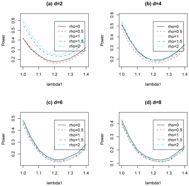
In order to study the effect of using controls in the statistical power of detecting associated SNPs, a Monte Carlo simulation study is used to compare the power performance of the overall chi-square tests with and without controls. In the simulation study, we consider the number of diseases d = 2, 4, 6, and 8 with 1,000 cases for each disease, and the ratio of number of controls to the number of cases in each diseases, ρ = 0, 0.5, 1, 1.5 and 2. Note that ρ = 0 is the case without controls. We assume Hardy-Weinberg Equilibrium (HWE) holds for controls and the minor allele frequency (maf) 0.1, 0.3 and 0.5 are considered. The genotype frequencies of the three genotypes for each disease and control are assumed to be trinomial distributed. For given genotype frequencies of controls, the relative risk of genotype AB to genotype AA (denoted as λ₁) and the relative risk of genotype BB to genotype AA (denoted as λ₂, the genotype frequencies for the three genotypes of the disease can be generated (see, for example, Chen, 2011; Chen and Ng, 2012). Various genetic models are considered in the simulation study. In particular, we consider λ₂ = 1.4 with λ₁ varies from 1.0 to 1.4 with increment 0.05. These settings cover several special genetic models, such as the dominant model (λ₁ = 1.4, λ₂ = 1.4), the recessive model (λ₁ = 1.0, λ₂ = 1.4), and the additive model (λ₁ = 1.2, λ₂ = 1.4). We assume that the SNPs are only associated with one of the d diseases. The significance level of the statistical test is set to be a = 10⁻³ and 10⁵ replications are used to estimate the type I error rates and power values of different test procedures.

3 Results

3.1 Real Data Example

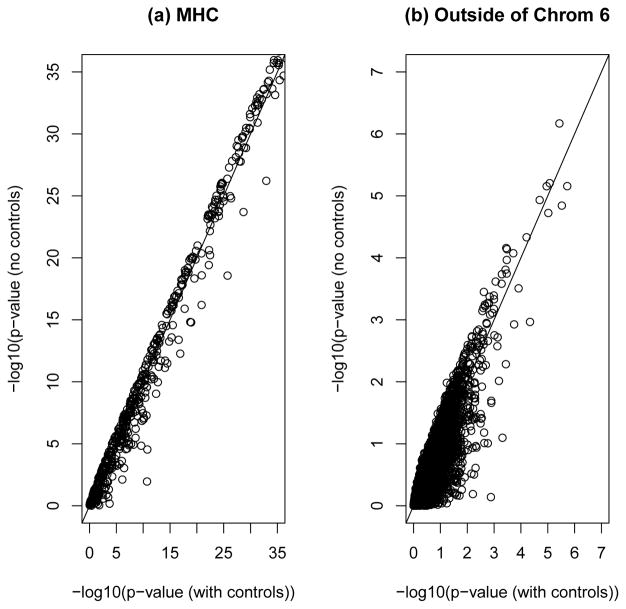
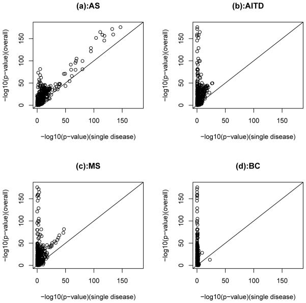
Based on the GWAS described in Section 2.2, we first compare the overall chi-square tests with and without controls when they are applied to MHC SNPs. Figure 1(a) plotted the negative log10 of the p-values from the two tests. For most of the MHC SNPs, the two tests give similar p-values. For those MHC SNPs with relatively smaller p-values from both tests, the p-values from the overall chi-square test without controls are usually smaller than the corresponding p-values from the overall chi-square test with controls. Then, we compare the overall chi-square test without controls with the CSP method which test associations based one each individual disease with the common controls (Chen, 2011). Figure 2 plotted the negative log10 p-values from the two methods applied to the four diseases. In most cases, we can observe that the overall test without controls gives smaller p-values than the CSP method applied to each disease. This indicates that the overall chi-square test without controls can detect associated SNPs more effectively than the CSP method applied to a single disease.

Fig. 1.

Negative log10 p-values from the overall chi-square tests with and without controls. (a) For MHC SNPs, (b) For nsSNPs outside of chromosome 6.

Fig. 2.

Negative log10 p-values for MHC SNPs from single CSP test (disease vs. control) and the overall chi-square test without controls (i.e., 4 diseases only).

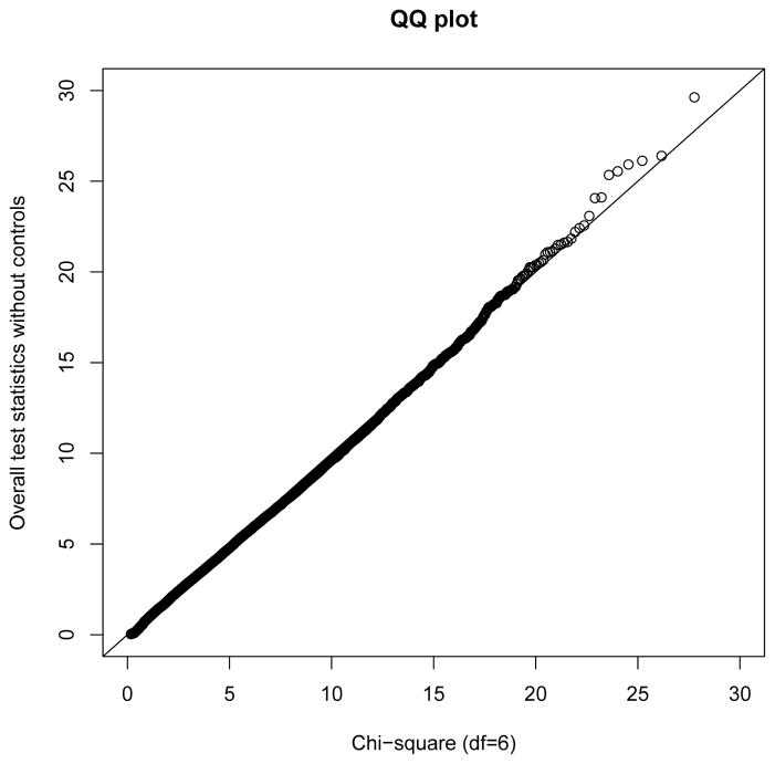
For nsSNPs outside of chromosome 6, the negative log10 p-values of the overall chi-square tests with and without controls are presented in Figure 1(b). Most of the nsSNPs had p-values larger than 10⁻³ from each test and there are only a few SNPs have small p-values from both tests. Figure 3 presents the quantile-quantile (QQ) plot of the test statistics obtained by the overall chi-square test without controls compared with a chi-square distribution with 6 df. It shows that except for some possible associated SNPs, the test statistic from the overall chi-square test without controls for nsSNPs outside of chromosome 6 follows a chi-square distribution.

Fig. 3.

Quantile-Quantile plot of the statistics from the overall chi-square test without controls for nsSNPs outside of chromosome 6 vs. a chi-square distribution with df = 6.

Table 1 listed 12 nsSNPs outside of chromosome 6 that have p-values less than 10⁻⁴ from either the overall chi-square tests with or without controls. The p-values from CSP method for individual disease with common controls of these 12 SNPs are also listed. Most of the confirmed associated SNPs (WTCCC & AAASC, 2007) were also found by the overall chi-square test without controls. However, the overall chi-square test without control also gives very small p-values for some SNPs which are not detected previously based on individual tests using common controls. For instance, SNP rs278981 has p-value 6.79 × 10⁻⁷ from the overall chi-square test without controls, while the p-values from tests based on each individual disease with shared controls are all larger than 0.01.

Table 1.

SNPs outside of chromosome 6 having p-values less than 10⁻⁴ from overall tests with or without controls.

SNP	Chrom	Location	CSP(AS)	CSP(ATD)	CSP(MS)	CSP(BC)	Overall χ2 test with controls	Overall χ2 test without controls
RS7522061	1	154481463	8.49E-02	1.57E-04	2.40E-01	8.20E-01	6.14E-05	4.66E-05
2RS278981	4	40268938	1.72E-01	1.89E-02	4.58E-02	7.84E-02	3.68E-06	6.79E-07
RS27044*	5	96144608	7.88E-07	7.75E-01	2.23E-01	1.00E+00	2.99E-06	1.44E-05
RS17482078*	5	96144622	7.93E-06	3.87E-01	2.62E-01	1.82E-01	2.01E-05	1.17E-05
RS10050860*	5	96147966	1.91E-06	5.03E-01	1.93E-01	1.98E-01	8.47E-06	6.25E-06
RS30187*	5	96150086	1.23E-06	1.78E-01	6.68E-02	1.00E+00	1.88E-06	6.97E-06
RS2287987*	5	96155291	2.18E-06	4.08E-01	2.65E-01	2.13E-01	1.10E-05	6.99E-06
RS11953798	5	177415724	1.66E-03	6.40E-01	2.94E-01	7.80E-01	4.58E-05	1.08E-03
RS3824419	9	1046728	8.69E-01	4.62E-01	1.94E-01	1.58E-02	3.52E-04	6.96E-05
RS727913	9	122457288	1.00E-02	9.97E-01	6.91E-03	2.16E-01	9.52E-06	1.89E-05
RS1935	10	64597829	1.04E-02	1.51E-01	8.62E-01	1.44E-02	3.31E-04	7.26E-05
RS7302230*	12	7179699	3.43E-04	4.26E-01	3.44E-01	4.84E-01	1.92E-04	8.44E-05

^*Confirmed by the original study.

CSP: chi-square partition method; AS: autoimmune diseases; AITD: autoimmune thyroid disease; MS: multiple sclerosis; BC: breast cancer.

3.2 Monte Carlo Simulation Study

Monte Carlo simulation study described in Section 2.3 is used to investigate the behaviors of the overall chi-square tests with and without controls. The estimated type I error rates of the overall chi-square tests with different maf, number of diseases d = 2, 4, 6, 8, and control-to-case ratio ρ = 0, 0.5, 1, 1.5, 2 are presented in Table 2. For all of the settings considered here, the estimated type I error rates were close to the prefixed significance level 10⁻³, which indicates that these statistical tests can well control the type I error rate close to the desired level.

Table 2.

Estimated type I error rates for varying maf, number of diseases (d), and control to case rate (ρ) from simulation with 10⁵ replications at significance level 10⁻³.

maf	d	ρ = 0	ρ = 0.5	ρ = 1	ρ = 1.5	ρ = 2
0.1	2	0.00064	0.00111	0.00083	0.00092	0.00088
	4	0.00094	0.00099	0.00108	0.00097	0.00122
	6	0.00114	0.00101	0.00107	0.00124	0.00112
	8	0.00110	0.00122	0.00100	0.00116	0.00109
0.3	2	0.00098	0.00086	0.00081	0.00085	0.00102
	4	0.00098	0.00094	0.00101	0.00103	0.00092
	6	0.00088	0.00105	0.00084	0.00097	0.00108
	8	0.00091	0.00095	0.00095	0.00079	0.00095
0.5	2	0.00098	0.00113	0.00104	0.00110	0.00110
	4	0.00093	0.00094	0.00095	0.00098	0.00098
	6	0.00099	0.00105	0.00092	0.00099	0.00103
	8	0.00102	0.00114	0.00111	0.00091	0.00104

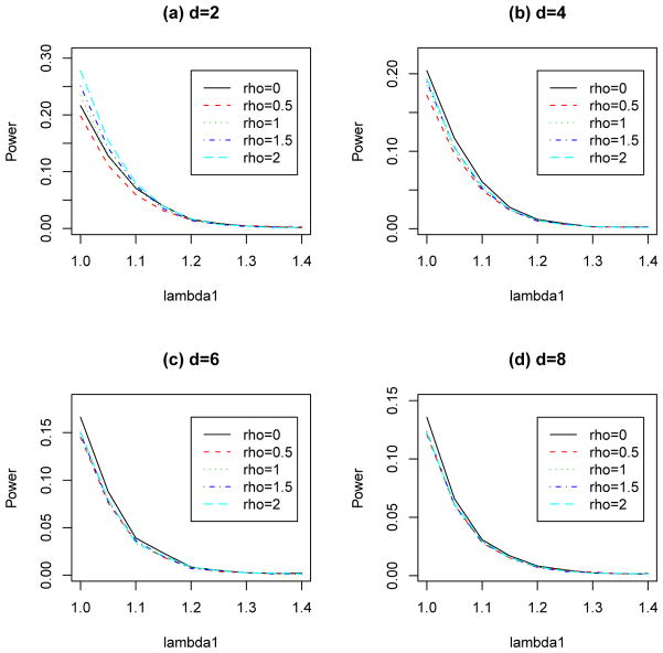
Then, we investigate the power properties of the overall chi-square tests with and without controls. The estimated power values for the overall chi-square tests with controls (ρ > 0) and without controls (ρ = 0) with maf = 0.1 and 0.5 are presented in Figure 4 and Figure 5, respectively. For the case with only two diseases (d = 2, see Figures 4(a) and 5(a)), we observe that the overall chi-square test without control (ρ = 0) is more powerful than the overall chi-square test with 500 controls (ρ = 0.5), but it is less powerful than the overall chi-square tests with 1000, 1500 and 2000 controls (ρ = 1, 1.5 and 2). For ρ ≥ 1, the power increases as the value of ρ increases. For the cases with four, six and eight diseases (d = 4, 6, 8, see Figure 4(b)–(d)), in most genetic models, the overall chi-square test without controls is the most powerful test compare to overall chi-square tests with controls. This illustrates that the use of controls may reduce the power in detecting associations under these settings. Note that we have also considered the case with mad = 0.3 and the situations when HWE does not hold for the control. Similar conclusions described above can be obtained, therefore, for the sake of reducing the length of the manuscript, the simulation results are not presented here.

Fig. 4.

Estimated power values of the overall chi-square tests with number of diseases d = 2, 4, 6, 8, each has 1,000 cases and different numbers of controls (1,000× ρ) at significance level 10⁻³. HWE with maf = 0.1 is assumed for controls.

Fig. 5.

Estimated power values of the overall chi-square tests with number of diseases d = 2, 4, 6, 8, each has 1,000 cases and different numbers of controls (1,000× ρ) at significance level 10⁻³. HWE with maf = 0.5 is assumed for controls.

Through simulation, Chen et al. (2012) have shown that the overall chi-square test with controls is more powerful than the tests using one case group with common or expanded controls (i.e., treating all other cases besides the disease of interest as controls). It has been shown that the power gain of the overall chi-square test can be drastic sometimes. Since the overall chi-square test proposed in this paper is usually outperforming the overall chi-square test with controls, therefore, it is also more powerful than other tests comparing cases with common or expanded controls.

4 Discussion

Our analyses have shown that the overall chi-square test is more powerful than the individual tests comparing single disease with shared controls in detecting associations. These results also confirm that GWAS with multiple diseases can be more efficient compare to GWAS with single disease.

When multiple diseases are considered simultaneously in GWAS, our results from the real data analysis and Monte Carlo simulation study suggest that GWAS without controls can be more efficient in terms of the power of the overall chi-square test. Moreover, the proposed overall chi-square test without control can well control the type I error rate close to the desired level. The power gain of the proposed overall chi-square test without controls is due to the fact that it has a smaller df than the chi-square test with controls. Compare to the usual case-control GWAS, the advantages of conducting GWAS with multiple diseases without controls are reducing the cost and time of the data collection process and increasing the power in detecting significant associations.

Although we gain in power while using the overall chi-square test without controls, there are several possible limitations of this study design and testing method in GWAS. First, without the controls, it may be difficult to identify which disease(s) is(are) associated with a SNP that is significant from the overall test. One of the possible solutions to this problem is to find the genotypic frequencies of healthy people (i.e., people without the diseases of interest) of the same population from previous studies if available, or genotype those “associated” SNPs (e.g., SNPs with small p-values from the overall test) from healthy people of the same population and then compare these data with each disease. Usually the number of “associated” SNPs in a GWAS is relatively much smaller than the total number of SNPs being studied, therefore, the cost of the extra genotyping for healthy people is relatively minor compare to the total cost. Second, another possible limitation for the proposed method is that the overall test will have no power if all the diseases in the study are associated with the genotype and have the same genetic models (i.e., same values of λ₁ and λ₂). However, this is not a major concern because this situation will rarely happen and it can be avoided by choosing unlinked diseases in the study. Third, the lack of ability to detect problematic SNPs which are deviated from HWE based on the control data could be another limitation of the proposed study design. Though, this issue can be solved similarly by using extra genotyping of the significant SNPs from healthy people of the same population.

It should be pointed out that many SNPs in a GWAS are correlated due to linkage disequilibrium. Consequently, the corresponding p-values of these correlated SNPs are also dependent. Some usual approaches to correct the significance level for multiple comparisons, such as Bonferroni method, may be too conservative and/or they may not control the family-wise error rate at the desired level. Different approaches have been proposed to solve this problem by estimating the cutoff p-value using the subject-level data (Churchill and Doerge, 1994; Cheverud, 2001; Li and Ji, 2005; Conneely and Boehnke, 2007; Dudbridge and Gusnanto, 2008; Gao et al., 2008; Moskvina and Schmidt, 2008; Pe’er et al., 2008; Chen and Liu, 2011). Further investigations are needed to find out which approach is better for the proposed overall chi-square test for GWAS with multiple diseases but no controls and we hope to report the findings in another manuscript.

Appendix: Sample Size Determination and Power Estimation

We have shown that the overall chi-square test without controls can be outperform the tests with controls when the number of diseases d ≥ 4. In planning GWAS with multiple diseases and no controls, it is important to determine the required sample size and/or estimate the power values. In this subsection, we present the formula for sample size determination and power estimation when the overall chi-square test is used to test for association in GWAS with multiple diseases and no controls. Under the alternative hypothesis, the overall chi-square test statistic without controls in (2) has an asymptotic non-central chi-square distribution with df 2d and a non-centrality parameter γ (Guenther, 1977).

Let us denote the genotypic frequency of genotype j (j = 1, 2, 3, which representing AA, AB, and BB, respectively) for disease i (i = 1, 2, …, d) under the alternative hypothesis as p_ij, and the genotypic frequency of genotype j as p_j . For a given alternative hypothesis, p_ij is known and p_j can be calculated by

$$p_j=\frac{n_1}{n}{p}_j^{(d)}+\left(1-\frac{n_1}{n}\right)p_j^{(0)},$$

where n₁ is the number of cases of associated disease (here we assume the first disease group is associated with the SNP), $p_j^{(0)}$ and $p_j^{(d)}$ are the genotypic frequency of genotype j under the null and alternative hypotheses, respectively. Usually, $p_j^{(d)}$ are calculated based on $p_j^{(0)}$ and relative risks (i.e., λ₁ and λ₂) using the following formulas (Chen, 2011; Chen and Ng, 2012):

$$\begin{array}{l}{p}_1^{(d)}=\frac{p_1^{(0)}}{p_1^{(0)}+{\lambda }_1{p}_2^{(0)}+{\lambda }_2{p}_3^{(0)}},\\ p_2^{(d)}=\frac{{\lambda }_1{p}_2^{(0)}}{p_1^{(0)}+{\lambda }_1{p}_2^{(0)}+{\lambda }_2{p}_3^{(0)}}\\ \text{and}{p}_3^{(d)}=\frac{{\lambda }_2{p}_3^{(0)}}{p_1^{(0)}+{\lambda }_1{p}_2^{(0)}+{\lambda }_2{p}_3^{(0)}}.\end{array}$$

Thus, the non-centrality parameter γ can be expressed as (Guenther, 1977):

$$\gamma =\sum _{i=1}^3\frac{1}{p_j}\left[\sum _{i=1}^d{c}_{ij}^2\frac{n_i}{n}-{\left(\sum _{i=1}^d{c}_{ij}\frac{n_i}{n}\right)}^2\right],$$ (3)

where n_i is the sample size for disease i, and n is the total sample size; c_ij satisfies

$$p_{ij}=p_j+\frac{c_{ij}}{\sqrt{n}}\text{and}\sum _{j=1}^3{c}_{ij}=0.$$

For a specific alternative hypothesis and a given significance level α, the power of the overall chi-square test without controls can be calculated as:

$$\text{Power}=Pr({\chi }_{2d}^2(\gamma )>{\chi }_{2d,1-\alpha }^2),$$ (4)

where ${\chi }_{2d,1-\alpha }^2$ is the (1 − α)th quantile of the chi-square distribution with df 2d and γ is the non-centrality parameter obtained from (3). Using numerical method, equation (4) can also be used to determine the required sample size for a pre-specified desired power value and fixed significance level.

References

- Armitage P. Tests for Linear Trends in Proportions and Frequencies. Biometrics. 1955;11:375–386. [Google Scholar]
- Chen Z. A New Association Test Based on Chi-Square Partition for Case-control GWA Studies. Genetic Epidemiology. 2011;35:658–663. doi: 10.1002/gepi.20615. [DOI] [PubMed] [Google Scholar]
- Chen Z, Huang H, Ng HKT. Testing for Association in Case Control GWAS with Shared Controls. 2012 doi: 10.1177/0962280212474061. unpublished manuscript. [DOI] [PubMed] [Google Scholar]
- Chen Z, Liu Q. A New Approach to Account for the Correlations among Single Nucleotide Polymorphisms in Genome-Wide Association Studies. Human Heredity. 2011;72:1–9. doi: 10.1159/000330135. [DOI] [PMC free article] [PubMed] [Google Scholar]
- Chen Z, Ng HKT. A Robust Method for Testing Association in Genome-wide Association Studies. Human Heredity. 2012;73:26–34. doi: 10.1159/000334719. [DOI] [PMC free article] [PubMed] [Google Scholar]
- Cheverud JM. A simple correction for multiple comparisons in interval mapping genome scans. Heredity. 2001;87:52–58. doi: 10.1046/j.1365-2540.2001.00901.x. [DOI] [PubMed] [Google Scholar]
- Churchill GA, Doerge RW. Empirical threshold values for quantitative trait mapping. Genetics. 1994;138:963–971. doi: 10.1093/genetics/138.3.963. [DOI] [PMC free article] [PubMed] [Google Scholar]
- Cochran W. Some methods for strengthening the common chi-square tests. Biometrics. 1954;10:417–451. [Google Scholar]
- Conneely KN, Boehnke M. So Many Correlated Tests, So Little Time! Rapid Adjustment of P Values for Multiple Correlated Tests. Am J Hum Genet. 2007;81:1158–1168. doi: 10.1086/522036. [DOI] [PMC free article] [PubMed] [Google Scholar]
- Craddock N, Hurles ME, Cardin N, Pearson RD, Plagnol V, Robson S, Vukcevic D, Barnes C, Conrad DF, Giannoulatou E. Genome-wide association study of CNVs in 16,000 cases of eight common diseases and 3,000 shared controls. Nature. 2010;464:713–720. doi: 10.1038/nature08979. [DOI] [PMC free article] [PubMed] [Google Scholar]
- Dudbridge F, Gusnanto A. Estimation of significance thresholds for genomewide association scans. Genet Epidemiol. 2008;32:227–234. doi: 10.1002/gepi.20297. [DOI] [PMC free article] [PubMed] [Google Scholar]
- Freidlin B, Zheng G, Li Z, Gastwirth JL. Trend tests for case-control studies of genetic markers: power, sample size and robustness. Hum Hered. 2002;53:146–152. doi: 10.1159/000064976. [DOI] [PubMed] [Google Scholar]
- Gao X, Starmer J, Martin ER. A multiple testing correction method for genetic association studies using correlated single nucleotide polymorphisms. Genet Epidemiol. 2008;32:361–369. doi: 10.1002/gepi.20310. [DOI] [PubMed] [Google Scholar]
- Guenther WC. Power and sample size for approximate chi-square tests. American Statistician. 1977;31:83–85. [Google Scholar]
- Li J, Ji L. Adjusting multiple testing in multilocus analyses using the eigenvalues of a correlation matrix. Heredity. 2005;95:221–227. doi: 10.1038/sj.hdy.6800717. [DOI] [PubMed] [Google Scholar]
- Moskvina V, Schmidt KM. On multiple-testing correction in genome-wide association studies. Genet Epidemiol. 2008;32:567–573. doi: 10.1002/gepi.20331. [DOI] [PubMed] [Google Scholar]
- Pe’er I, Yelensky R, Altshuler D, Daly MJ. Estimation of the multiple testing burden for genomewide association studies of nearly all common variants. Genet Epidemiol. 2008;32:381–385. doi: 10.1002/gepi.20303. [DOI] [PubMed] [Google Scholar]
- The Wellcome Trust Case Control Consortium. Genome-wide association study of 14,000 cases of seven common diseases and 3,000 shared controls. Nature. 2007;447:661–678. doi: 10.1038/nature05911. [DOI] [PMC free article] [PubMed] [Google Scholar]
- The Wellcome Trust Case Control Consortium & The Australo-Anglo-American Spondylitis Consortium. Association scan of 14,500 nonsynonymous SNPs in four diseases identifies autoimmunity variants. Nat Genet. 2007;39:1329–1337. doi: 10.1038/ng.2007.17. [DOI] [PMC free article] [PubMed] [Google Scholar]
- Zheng G, Ng HKT. Genetic model selection in two-phase analysis for case-control association studies. Biostatistics. 2008;9:391–399. doi: 10.1093/biostatistics/kxm039. [DOI] [PMC free article] [PubMed] [Google Scholar]