Statistical detection of systematic election irregularities

Abstract

Democratic societies are built around the principle of free and fair elections, and that each citizen’s vote should count equally. National elections can be regarded as large-scale social experiments, where people are grouped into usually large numbers of electoral districts and vote according to their preferences. The large number of samples implies statistical consequences for the polling results, which can be used to identify election irregularities. Using a suitable data representation, we find that vote distributions of elections with alleged fraud show a kurtosis substantially exceeding the kurtosis of normal elections, depending on the level of data aggregation. As an example, we show that reported irregularities in recent Russian elections are, indeed, well-explained by systematic ballot stuffing. We develop a parametric model quantifying the extent to which fraudulent mechanisms are present. We formulate a parametric test detecting these statistical properties in election results. Remarkably, this technique produces robust outcomes with respect to the resolution of the data and therefore, allows for cross-country comparisons.

Free and fair elections are the cornerstone of every democratic society (1). A central characteristic of elections being free and fair is that each citizen’s vote counts equal. However, Joseph Stalin believed that “[i]t’s not the people who vote that count; it’s the people who count the votes.” How can it be distinguished whether an election outcome represents the will of the people or the will of the counters?

Elections can be seen as large-scale social experiments. A country is segmented into a usually large number of electoral units. Each unit represents a standardized experiment, where each citizen articulates his/her political preference through a ballot. Although elections are one of the central pillars of a fully functioning democratic process, relatively little is known about how election fraud impacts and corrupts the results of these standardized experiments (2, 3).

There is a plethora of ways of tampering with election outcomes (for instance, the redrawing of district boundaries known as gerrymandering or the barring of certain demographics from their right to vote). Some practices of manipulating voting results leave traces, which may be detected by statistical methods. Recently, Benford’s law (4) experienced a renaissance as a potential election fraud detection tool (5). In its original and naive formulation, Benford’s law is the observation that, for many real world processes, the logarithm of the first significant digit is uniformly distributed. Deviations from this law may indicate that other, possibly fraudulent mechanisms are at work. For instance, suppose a significant number of reported vote counts in districts is completely made up and invented by someone preferring to pick numbers, which are multiples of 10. The digit 0 would then occur much more often as the last digit in the vote counts compared with uncorrupted numbers. Voting results from Russia (6), Germany (7), Argentina (8), and Nigeria (9) have been tested for the presence of election fraud using variations of this idea of digit-based analysis. However, the validity of Benford’s law as a fraud detection method is subject to controversy (10, 11). The problem is that one needs to firmly establish a baseline of the expected distribution of digit occurrences for fair elections. Only then it can be asserted if actual numbers are over- or underrepresented and thus, suspicious. What is missing in this context is a theory that links specific fraud mechanisms to statistical anomalies (10).

A different strategy for detecting signals of election fraud is to look at the distribution of vote and turnout numbers, like the strategy in ref. 12. This strategy has been extensively used for the Russian presidential and Duma elections over the last 20 y (13–15). These works focus on the task of detecting two mechanisms, the stuffing of ballot boxes and the reporting of contrived numbers. It has been noted that these mechanisms are able to produce different features of vote and turnout distributions than those features observed in fair elections. For Russian elections between 1996 and 2003, these features were only observed in a relatively small number of electoral units, and they eventually spread and percolated through the entire Russian federation from 2003 onward. According to the work by Myagkov and Ordeshook (14), “[o]nly Kremlin apologists and Putin sycophants argue that Russian elections meet the standards of good democratic practice.” This point was further substantiated with election results from the 2011 Duma and 2012 presidential elections (16–18). Here, it was also observed that ballot stuffing not only changes the shape of vote and turnout distributions but also induces a high correlation between them. Unusually high vote counts tend to co-occur with unusually high turnout numbers.

Several recent advances in the understanding of statistical regularities of voting results are caused by the application of statistical physics concepts to quantitative social dynamics (19). In particular, several approximate statistical laws of how vote and turnout are distributed have been identified (20–22), and some of them are shown to be valid across several countries (23, 24). It is tempting to think of deviations from these approximate statistical laws as potential indicators for election irregularities, which are valid cross-nationally. However, the magnitude of these deviations may vary from country to country because of different numbers and sizes of electoral districts. Any statistical technique quantifying election anomalies across countries should not depend on the size of the underlying sample or its aggregation level (i.e., the size of the electoral units). As a consequence, a conclusive and robust signal for a fraudulent mechanism (e.g., ballot stuffing) must not disappear if the same dataset is studied on different aggregation levels.

In this work, we expand earlier work on statistical detection of election anomalies in two directions. We test for reported statistical features of voting results (and deviations thereof) in a cross-national setting and discuss their dependence on the level of data aggregation. As the central point of this work, we propose a parametric model to statistically quantify to which extent fraudulent processes, such as ballot stuffing, may have influenced the observed election results. Remarkably, under the assumption of coherent geographic voting patterns (24, 25), the parametric model results do not depend significantly on the aggregation level of the election data or the size of the data sample.

Data and Methods

Election Data.

Countries were selected by data availability. For each country, we require availability of at least one aggregation level where the average population per territorial unit . This limit for was chosen to include a large number of countries that have a comparable level of data resolution. We use data from recent parliamentary elections in Austria, Canada, Czech Republic, Finland, Russia (2011), Spain, and Switzerland, the European Parliament elections in Poland, and presidential elections in France, Romania, Russia (2012), and Uganda. Here, we refer by unit to any incarnation of an administrative boundary (such as districts, precincts, wards, municipals, provinces, etc.) of a country on any aggregation level. If the voting results are available on different levels of aggregation, we refer to them by Roman numbers (i.e., Poland-I refers to the finest aggregation level for Poland, Poland-II to the second finest aggregation level, and so on). For each unit on each aggregation level for each country, we have the data of the number of eligible persons to vote, valid votes, and votes for the winning party/candidate. Voting results were obtained from official election homepages of the respective countries (Table S1). Units with an electorate smaller than 100 are excluded from the analysis to prevent extreme turnout and vote rates as artifacts from very small communities. We tested robustness of our findings with respect to the choice of a minimal electorate size and found that the results do not significantly change if the minimal size is set to 500.

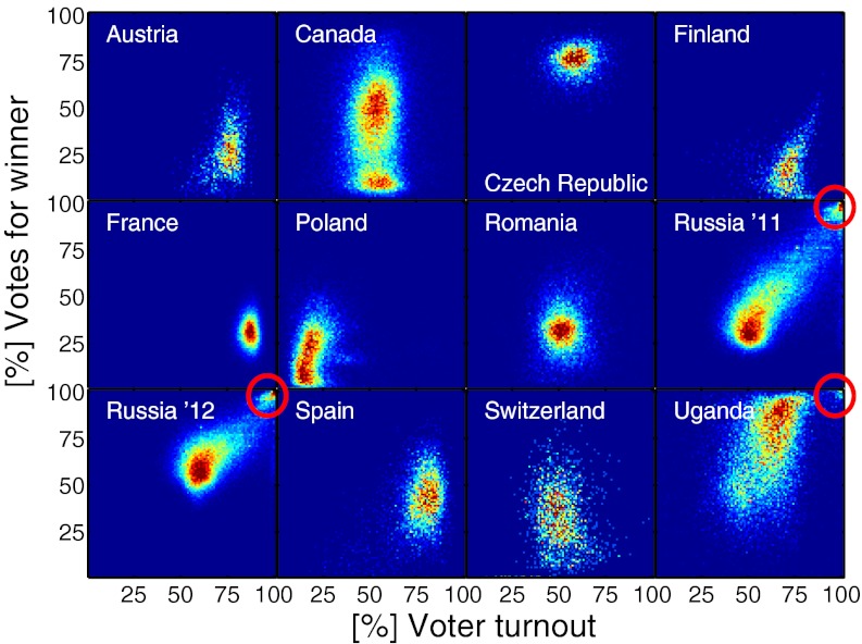
The histograms for the 2-d vote turnout distributions (vtds) for the winning parties, also referred to as “fingerprints,” are shown in Fig. 1.

Fig. 1.

Election fingerprints. Two-dimensional histograms of the number of units for a given voter turnout (x axis) and the percentage of votes (y axis) for the winning party (or candidate) in recent elections from different countries (Austria, Canada, Czech Republic, Finland, France, Poland, Romania, Russia 2011, Russia 2012, Spain, Switzerland, and Uganda) are shown. Color represents the number of units with corresponding vote and turnout numbers. The units usually cluster around a given turnout and vote percentage level. In Uganda and Russia, these clusters are smeared out to the upper right region of the plots, reaching a second peak at a 100% turnout and 100% of votes (red circles). In Canada, there are clusters around two different vote values, corresponding to the Québécois and English Canada (SI Text). In Finland, the main cluster is smeared out into two directions (indicative of voter mobilization because of controversies surrounding the True Finns).

Data Collapse.

It has been shown that, by using an appropriate rescaling of election data, the distributions of votes and turnouts approximately follow a Gaussian distribution (24). Let W_i be the number of votes for the winning party and N_i be the number of voters in any unit i. A rescaling function is given by the logarithmic vote rate (24). In units where W_i ≥ N_i (because of errors in counting or fraud) or W_i = 0, ν_i is not defined, and the unit is omitted from our analysis. This definition is conservative, because districts with extreme but feasible vote and turnout rates are neglected (for instance, in Russia in 2012, there are 324 units with 100% vote and 100% turnout).

Parametric Model.

To motivate our parametric model for the vtd, observe that the vtd for Russia and Uganda in Fig. 1 are clearly bimodal in both turnout and votes. One cluster is at intermediate levels of turnout and votes. Note that it is smeared toward the upper right parts of the plot. The second peak is situated in the vicinity of the 100% turnout and 100% votes point. This peak suggests that two modes of fraud mechanisms are present: incremental and extreme fraud. Incremental fraud means that, with a given rate, ballots for one party are added to the urn and/or votes for other parties are taken away. This fraud occurs within a fraction f_i of units. In the election fingerprints in Fig. 1, these units are associated with the smearing to the upper right side. Extreme fraud corresponds to reporting a complete turnout and almost all votes for a single party. This fraud happens in a fraction f_e of units and forms the second cluster near 100% turnout and votes for the winning party.

For simplicity, we assume that, within each unit, turnout and voter preferences can be represented by a Gaussian distribution, with the mean and SD taken from the actual sample (Fig. S1). This assumption of normality is not valid in general. For example, the Canadian election fingerprint of Fig. 1 is clearly bimodal in vote preferences (but not in turnout). In this case, the deviations from approximate Gaussianity are because of a significant heterogeneity within the country. In the particular case of Canada, this heterogeneity is known to be due to the mix of the Anglo- and Francophone population. Normality of the observed vote and turnout distributions is discussed in Table S2.

Let V_i be the number of valid votes in unit i. The first step in the model is to compute the empirical turnout distribution, V_i/N_i, and the empirical vote distribution, W_i/N_i, over all units from the election data. To compute the model vtd, the following protocol is then applied to each unit i.

• i) For each i, take the electorate size N_i from the election data.

• ii) Model turnout and vote rates for i are drawn from normal distributions. The mean of the model turnout (vote) distribution is estimated from the election data as the value that maximizes the empirical turnout (vote) distribution. The model variances are also estimated from the width of the empirical distributions (details in SI Text and Fig. S1).

• iii) Incremental fraud. With probability f_i, ballots are taken away from both the nonvoters and the opposition, and they are added to the winning party’s ballots. The fraction of ballots that is shifted to the winning party is again estimated from the actual election data.

• iv) Extreme fraud. With probability f_e, almost all ballots from the nonvoters and the opposition are added to the winning party’s ballots.

The first step of the above protocol ensures that the actual electorate size numbers are represented in the model. The second step guarantees that the overall dispersion of vote and turnout preferences of the country’s population are correctly represented in the model. Given nonzero values for f_i and f_e, incremental and extreme fraud are then applied in the third and fourth step, respectively. Complete specification of these fraud mechanisms is in SI Text.

Estimating the Fraud Parameters.

Values for f_i and f_e are reverse-engineered from the election data in the following way. First, model vtds are generated according to the above scheme for each combination of (f_i, f_e) values, where f_i and f_e ∈ {0, 0.01, 0.02, … 1}. We then compute the pointwise sum of the square difference of the model and observed vote distributions for each pair (f_i, f_e) and extract the pair giving the minimal difference. This procedure is repeated for 100 iterations, leading to 100 pairs of fraud parameters (f_i, f_e). In Results, we report the average values of these f_i and f_e values, respectively, and their SDs. More details are in SI Text.

Results

Fingerprints.

Fig. 1 shows 2-d histograms (vtds) for the number of units for a given fraction of voter turnout (x axis) and the percentage of votes for the winning party (y axis). Results are shown for Austria, Canada, Czech Republic, Finland, France, Poland, Romania, Russia, Spain, Switzerland, and Uganda. For each of these countries, the data are shown on the finest aggregation level, where . These figures can be interpreted as fingerprints of several processes and mechanisms, leading to the overall election results. For Russia and Uganda, the shape of these fingerprints differs strongly from the other countries. In particular, there is a large number of territorial units (thousands) with ∼100% turnout and at the same time, ∼100% of votes for the winning party.

Approximate Normality.

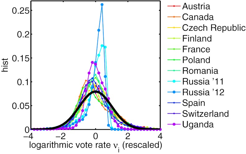
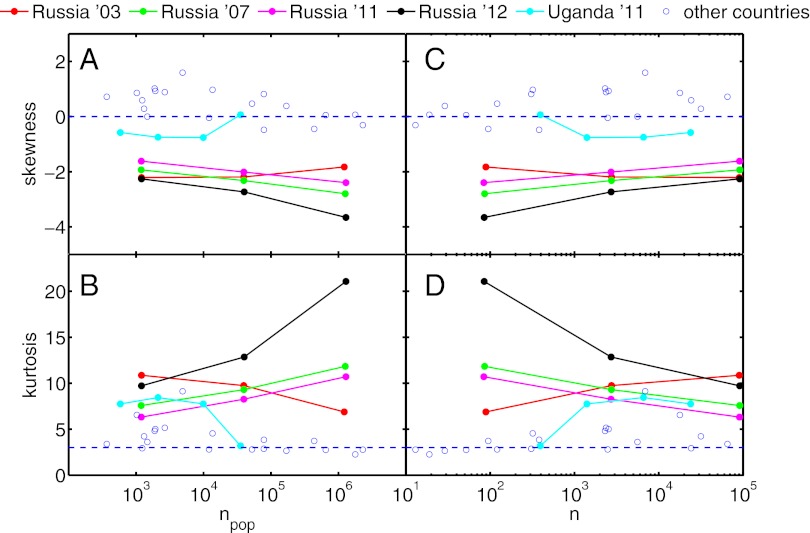
In Fig. 2, we show the distribution of ν_i for each country. Roughly, to first order, the data from different countries collapse to an approximate Gaussian distribution as previously observed (24). Clearly, the data for Russia fall out of line. Skewness and kurtosis for the distributions of ν_i are listed for each dataset and aggregation level in Table S3. Most strikingly, the kurtosis of the distributions for Russia (2003, 2007, 2011, and 2012) exceeds the kurtosis of each other country on the coarsest aggregation level by a factor of two to three. Values for the skewness of the logarithmic vote rate distributions for Russia are also persistently below the values for each other country. Note that, for the vast majority of the countries, skewness and kurtosis for the distribution of ν_i are in the vicinity of zero and three, respectively (which are the values that one would expect for normal distributions). However, the moments of the distributions do depend on the data aggregation level. Fig. 3 shows skewness and kurtosis for the distributions of ν_i for each election on each aggregation level. By increasing the data resolution, skewness and kurtosis for Russia decrease and approach similar values to the values observed in the rest of the countries (Table S3). These measures depend on the data resolution and thus, cannot be used as unambiguous signals for statistical anomalies. As will be shown, the fraud parameters f_i and f_e do not significantly depend on the aggregation level or total sample size.

Fig. 2.

A simple way to compare data from different elections in different countries on a similar aggregation level is to present the distributions of the logarithmic vote rates ν_i of the winning parties as rescaled distributions with zero mean and unit variance (24). Large deviations from other countries can be seen for Uganda and Russia with the plain eye. More detailed results are found in Table S3.

Fig. 3.

For each country on each aggregation level, skewness and kurtosis of the logarithmic vote rate distributions are shown as a function of the average electorate per unit in A and B, respectively, and as a function of the number of units n in C and D. Results for Russia and Uganda are highlighted. The values for all other countries cluster around zero and three, which are the values expected for normal distributions. On the largest aggregation level, election data from Uganda and Russia cannot be distinguished from other countries.

Voting Model Results.

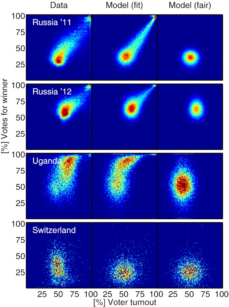
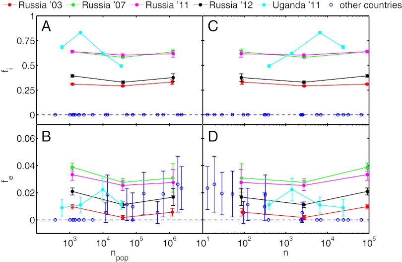
Estimation results for f_i and f_e are given in Table S3 for all countries on each aggregation level. They are zero (or almost zero) in all of the cases except for Russia and Uganda. In Fig. 4, Right, we show the model results for Russia (2011 and 2012), Uganda, and Switzerland for f_i = f_e = 0. The case where both fraud parameters are zero corresponds to the absence of incremental and extreme fraud mechanisms in the model and can be called the fair election case. In Fig. 4, Center, we show results for the estimated values of f_i and f_e. Fig. 4, Left shows the actual vtd of the election. Values of f_i and f_e significantly larger than zero indicate that the observed distributions may be affected by fraudulent actions. To describe the smearing from the main peak to the upper right corner, which is observed for Russia and Uganda, an incremental fraud probability around f_i = 0.64(1) is needed for United Russia in 2011 and f_i = 0.39(1) is needed in 2012. This finding means fraud in about 64% of the units in 2011 and 39% in 2012. In the second peak close to 100% turnout, there are roughly 3,000 units with 100% of votes for United Russia in the 2011 data, representing an electorate of more than 2 million people. Best fits yield f_e = 0.033(4) for 2011 and f_e = 0.021(3) for 2012 (i.e., 2–3% of all electoral units experience extreme fraud). A more detailed comparison of the model performance for the Russian parliamentary elections of 2003, 2007, 2011, and 2012 is found in Fig. S2. Fraud parameters for the Uganda data in Fig. 4 are found to be f_i = 0.49(1) and f_e = 0.011(3). A best fit for the election data from Switzerland gives f_i = f_e = 0.

Fig. 4.

Comparison of observed and modeled vtds for Russia 2011, Russia 2012, Uganda, and Switzerland. Left shows the observed election fingerprints. Center shows a fit with the fraud model. Right shows the expected model outcome of fair elections (i.e., absence of fraudulent mechanisms f_i = f_e = 0). For Switzerland, the fair and fitted models are almost the same. The results for Russia and Uganda can be explained by the model assuming a large number of fraudulent units.

These results are drastically more robust to variations of the aggregation level of the data than the previously discussed distribution moments skewness and kurtosis (Fig. 5 and Table S3). Even if we aggregate the Russian data up to the coarsest level of federal subjects (∼85 units, depending on the election), f_e estimates are still at least 2 SDs above zero and f_i estimates more than 10 SDs. Similar observations hold for Uganda. For no other country and no other aggregation level are such deviations observed. The parametric model yields similar results for the same data on different levels of aggregation as long as the values maximizing the empirical vote (turnout) distribution and the distribution width remain invariant. In other words, as long as units with similar vote (turnout) characteristics are aggregated to larger units, the overall shapes of the empirical distribution functions are preserved, and the model estimates do not change significantly. Note that more detailed assumptions about possible mechanisms leading to large heterogeneity in the data (such as the Québécois in Canada or voter mobilization in the Helsinki region in Finland) (SI Text) may have an effect on the estimate of f_i. However, these assumptions can, under no circumstances, explain the mechanism of extreme fraud. Results for elections in Sweden, the United Kingdom, and the United States, where voting results are only available on a much coarser resolution (), are given in Table S4.

Fig. 5.

For each country on each aggregation level, the values for f_i and f_e as given in Table S3 are shown as a function of the average electorate per unit in A and B, and for the number of units n in C and D, respectively. Results for Russia and Uganda are highlighted. The values for all other countries are close to zero, indicating that the data are best described by the absence of the ballot stuffing mechanism. Parameter values for f_i and f_e for Russia and Uganda remain significantly above zero for all aggregation levels. Note that, in D, the error margins for f_e values in the range 10 < n < 100 (as well as for the corresponding values f_e in C) get increasingly large, whereas f_i estimates in this range stay robust.

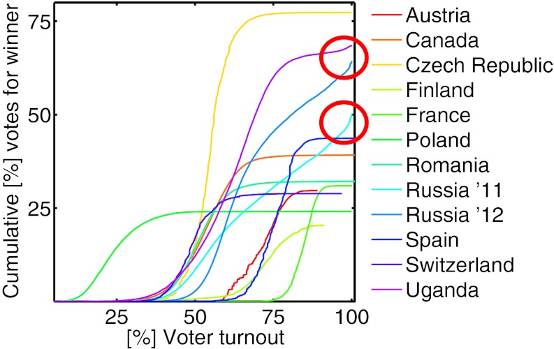
Another way to visualize the intensity of election irregularities is the cumulative number of votes as a function of the turnout (Fig. 6). For each turnout level, the total number of votes from units with this level or lower is shown. Each curve corresponds to the respective election winner in a different country with average electorate per unit of comparable order of magnitude. Usually, these cumulative distribution functions (cdfs) level off and form a plateau from the party’s maximal vote count. Again, this result is not the case for Russia and Uganda. Both show a boost phase of increased extreme fraud toward the right end of the distribution (red circles). Russia never even shows a tendency to form a plateau. As long as the empirical vote distribution functions remain invariant under data aggregation (as discussed above), the shape of these cdfs will be preserved as well. Note that Fig. 6 shows that these effects are decisive for winning the 50% majority in Russia in 2011.

Fig. 6.

The ballot stuffing mechanism can be visualized by considering the cumulative number of votes as a function of turnout. Each country’s election winner is represented by a curve, which typically takes the shape of a sigmoid function reaching a plateau. In contrast to the other countries, Russia and Uganda do not tend to develop this plateau but instead, show a pronounced increase (boost) close to complete turnout. Both irregularities are indicative of the two ballot stuffing modes being present.

Discussion

We show that it is not sufficient to discuss the approximate normality of turnout, vote, or logarithmic vote rate distributions to decide if election results may be corrupted. We show that these methods can lead to ambiguous signals, because results depend strongly on the aggregation level of the election data. We developed a model to estimate parameters quantifying to which extent the observed election results can be explained by ballot stuffing. The resulting parameter values are shown to be insensitive to the choice of the aggregation level. Note that the error margins for f_e values start to increase by decreasing n below 100 (Fig. 5D), whereas f_i estimates stay robust, even for very small n.

It is imperative to emphasize that the shape of the fingerprints in Fig. 1 will deviate from pure 2-d Gaussian distributions as a result of nonfraudulent mechanisms as well because of heterogeneity in the population. The purpose of the parametric model is to quantify to which extent ballot stuffing and the mechanism of extreme fraud may have contributed to these deviations or if their influence can be ruled out on the basis of the data. For the elections in Russia and Uganda, they cannot be ruled out. As shown in Fig. S2, assumptions of their widespread occurrences even allow us to reproduce the observed vote distributions to a good degree.

In conclusion, it can be said with almost certainty that an election does not represent the will of the people if a substantial fraction (f_e) of units reports a 100% turnout with almost all votes for a single party and/or if any significant deviations from the sigmoid form in the cumulative distribution of votes vs. turnout are observed. Another indicator of systematic fraudulent or irregular voting behavior is an incremental fraud parameter f_i, which is significantly greater than zero on each aggregation level.

Should such signals be detected, it is tempting to invoke G. B. Shaw, who held that “[d]emocracy is a form of government that substitutes election by the incompetent many for appointment by the corrupt few.”

References

- 1.Diamond LJ, Plattner MF. Electoral Systems and Democracy. Baltimore: Johns Hopkins Univ Press; 2006. [Google Scholar]
- 2.Lehoucq F. Electoral fraud: Causes, types and consequences. Annu Rev Polit Sci. 2003;6:233–256. [Google Scholar]
- 3.Alvarez RM, Hall TE, Hyde SD. Election Fraud: Detecting and Deterring Electoral Manipulations. Washington, DC: Brookings Institution Press; 2008. [Google Scholar]
- 4.Benford F. The law of anomalous numbers. Proc Am Philos Soc. 1938;78:551–572. [Google Scholar]
- 5.Mebane WR. 2006. Election Forensics: Vote Counts and Benford's Law. (Political Methodology Society, University of California, Davis, CA)
- 6.Mebane WR, Kalinin K. 2009. Comparative Election Fraud Detection. (The American Political Science Association, Toronto, ON, Canada)
- 7.Breunig C, Goerres A. Searching for electoral irregularities in an established democracy: Applying Benford’s Law tests to Bundestag elections in unified Germany. Elect Stud. 2011;30:534–545. [Google Scholar]
- 8.Cantu F, Saiegh SM. Fraudulent democracy? An analysis of Argentina’s infamous decade using supervised machine learning. Polit Anal. 2011;19:409–433. [Google Scholar]
- 9.Beber B, Scacco A. What the numbers say: A digit-based test for election fraud. Polit Anal. 2012;20:211–234. [Google Scholar]
- 10.Deckert JD, Myagkov M, Ordeshook PC. Benford’s Law and the detection of election fraud. Polit Anal. 2011;19:245–268. [Google Scholar]
- 11.Mebane WR. Comment on “Benford’s Law and the detection of election fraud”. Polit Anal. 2011;19:269–272. [Google Scholar]
- 12.Mebane WR, Sekhon JS. Robust estimation and outlier detection for overdispersed multinomial models of count data. Am J Polit Sci. 2004;48:392–411. [Google Scholar]
- 13.Sukhovolsky VG, Sobyanin AA. Vybory i referendom 12 dekabrya 1993 g. v. Rossii: Politicheskie itogi, perskeptivy, dostovemost rezultatov. Moscow, Russia: Moksva-Arkhangelskoe; 1994. [Google Scholar]
- 14.Myagkov M, Ordeshook PC. Russian Election: An Oxymoron of Democracy. 2008. (VTP WP 63, California Institute of Technology, Pasadena, CA, and Massachusetts Institute of Technology, Cambridge, MA) [Google Scholar]
- 15.Myagkov M, Ordershook PC, Shakin D. Russia and Ukraine. Fraud or fairytales: Russia and Ukraine’s electoral experience. Post Soviet Affairs. 2005;21:91–131. [Google Scholar]
- 16.Shpilkin S. Statistical investigation of the results of Russian elections in 2007–2009. Troitskij Variant. 2009;21:2–4. [Google Scholar]
- 17.Shpilkin S. Mathematics of elections, Troitskij Variant. 2011;40:2–4. [Google Scholar]
- 18.Kobak D, Shpilkin S, Pshenichnikov MS. Statistical anomalies in 2011–2012 Russian elections revealed by 2D correlation analysis, arXiv:1205.0741v2 [physics.soc-ph] 2012 [Google Scholar]
- 19.Castellano C, Fortunato S, Loreto V. Statistical physics of social dynamics. Rev Mod Phys. 2009;81:591–646. [Google Scholar]
- 20.Costa Filho RN, Almeida MP, Moreira JE, Andrade JS., Jr Brazilian elections: Voting for a scaling democracy. Physica A. 2003;322:698–700. [Google Scholar]
- 21.Lyra ML, Costa UMS, Costa Filho RN, Andrade JS., Jr Generalized Zipf’s law in proportional voting processes. Europhys Lett. 2003;62:131–135. [Google Scholar]
- 22.Mantovani MC, Ribeiro HV, Moro MV, Picoli S, Jr, Mendes RS. Scaling laws and universality in the choice of election candidates. Europhys Lett. 2011;96:48001–48005. [Google Scholar]
- 23.Fortunato S, Castellano C. Scaling and universality in proportional elections. Phys Rev Lett. 2007;99:138701. doi: 10.1103/PhysRevLett.99.138701. [DOI] [PubMed] [Google Scholar]
- 24.Borghesi C, Bouchaud JP. Spatial correlations in vote statistics: A diffusive field model for decision-making. Eur Phys J B. 2010;75:395–404. [Google Scholar]
- 25.Agnew J. Mapping politics: How context counts in electoral geography. Polit Geogr. 1996;15:129–146. [Google Scholar]
Associated Data
This section collects any data citations, data availability statements, or supplementary materials included in this article.