A novel missense-mutation-related feature extraction scheme for ‘driver’ mutation identification

Abstract

Motivation: It becomes widely accepted that human cancer is a disease involving dynamic changes in the genome and that the missense mutations constitute the bulk of human genetic variations. A multitude of computational algorithms, especially the machine learning-based ones, has consequently been proposed to distinguish missense changes that contribute to the cancer progression (‘driver’ mutation) from those that do not (‘passenger’ mutation). However, the existing methods have multifaceted shortcomings, in the sense that they either adopt incomplete feature space or depend on protein structural databases which are usually far from integrated.

Results: In this article, we investigated multiple aspects of a missense mutation and identified a novel feature space that well distinguishes cancer-associated driver mutations from passenger ones. An index (DX score) was proposed to evaluate the discriminating capability of each feature, and a subset of these features which ranks top was selected to build the SVM classifier. Cross-validation showed that the classifier trained on our selected features significantly outperforms the existing ones both in precision and robustness. We applied our method to several datasets of missense mutations culled from published database and literature and obtained more reasonable results than previous studies.

Availability: The software is available online at http://www.methodisthealth.com/software and https://sites.google.com/site/drivermutationidentification/.

Contact: xzhou@tmhs.org

Supplementary information: Supplementary data are available at Bioinformatics online.

1 INTRODUCTION

Human malignancies are believed to arise as a result of somatic alterations within the cancer genome that leads to activation of oncogenes or inactivation of tumor suppressor genes (Hanahan and Weinberg, 2000; Stratton et al., 2009; Weinberg, 2002, 2006; Weir et al., 2004). With the recent considerable improvement in genome analysis technologies, diverse alterations including point mutations, copy number increases and decreases, loss of allelic heterozygosity and chromosome translocations in the genome of a particular cancer type have gradually been specified. Among these, the missense mutations (a point mutation that results in a codon coding for a different amino acid) attract increasing attentions in that they are recurrently identified within the cancer genomes (Jones et al., 2008; Krawczak et al., 2000; Parsons et al., 2008; Sjoblom et al., 2006). Although up to hundreds of missense mutations were characterized in the genome of some cancer type [e.g. brain, breast, colorectal and pancreatic cancers, see http://www.sanger.ac.uk/genetics/CGP/cosmic/ and also (Jones et al., 2008)], only a small fraction of these mutations are suggested to directly contribute to the neoplastic process (‘driver’ mutation), whereas the remaining bulk consists of neutral polymorphisms which are believed to have no direct effect on the tumorigenesis (‘passenger’ mutation) (Stratton et al., 2009; Wood et al., 2007).

Differentiating driver mutation and passenger mutations is critical for understanding the molecular mechanisms responsible for cancer progression and also provides prognostic and diagnostic markers as well as targets for therapeutic interventions. However, the ability to distinguish these drivers is seriously limited by in vivo functional analyses alone. Therefore, this situation has provoked a bunch of mathematical methods that assist in prioritizing potential drivers for further analysis during the past years. These methods can be mainly categorized into two classes, the statistical method and the machine learning-based method. The former is largely based on the assumption that mutations that occur more frequently are more likely to be a driver mutation [e.g. (Greenman et al., 2006; Parmigiani et al., 2007)], which turned out to be somehow unreasonable according to recent reports, for example, Wood et al. (2007) pointed that it is the ‘hills’ (infrequently mutant genes) not the ‘mountains’ (frequently mutant genes) that dominate the cancer genome landscape. For the machine learning-based method, on the other hand, researchers typically extract features related to the missense mutations, train a classifier using label-clear mutations and perform classifications for the unknowns on the trained classifier. Through this routine, several groups have reported their results so far (Carter et al., 2009; Krishnan and Westhead, 2003; Ng and Henikoff, 2001; Ng and Henikoff, 2002; Sjoblom et al., 2006) and claimed their performance is better than others based on different classifier tools, training data and, particularly, on different feature spaces.

The existing machine learning-based methods have shortcomings on several aspects, especially on the feature space they employ to construct the classifier. For example, in Carter et al. (2009) and Krishnan and Westhead (2003), features relating to physicochemical properties of amino acids and structural traits of proteins are predicted using computational software. The reliability as well as significance of such kind of features are dubious (Krishnan and Westhead, 2003). Others may avoid the predicted attributes by relying on the published databases that contain structural traits or annotations they need (Jones et al., 2008; Sunyaev et al., 2001). The applicability of these models is limited because of the probable incompleteness of their cited databases. The remaining work avoids the above flaws at the price of missing some important properties of the mutation under investigation—they set up too simple rules for discrimination (Kaminker et al., 2007; Ng and Henikoff, 2001). The shortcomings mentioned here make questionable the reliability and/or robustness of prediction of the existing methods.

In this article, we comprehensively investigated the properties relating to a particular missense mutation. Besides the previously used features such as physicochemical changes upon the amino acid substitution and binary categorical features extracted from public annotated databases, we for the first time systematically studied all kinds of substitution scoring matrix (SSM) features and protein sequence-specific (PSS) features to evaluate their potential power of discrimination (see Section 2). A SSM (or mutation matrix) is typically a 20 × 20 numerical matrix with each element representing the similarity and distance of a particular pair of amino acids with respect to a particular physicochemical or biochemical property (Kawashima et al., 2008), making it potentially a candidate feature for discrimination. Some researchers (e.g. Carter et al., 2009; Jones et al., 2008) have incorporated several well-known substitution matrices such as PAM (Dayhoff et al., 1978), BLOSUM (Henikoff and Henikoff, 1992) and Grantham Score (Grantham, 1974) as predictive features, but is much incomplete. We explored many such substitution scoring matrices as candidate features and assessed their distinguishing capability. The PSS features were widely overlooked in the previous related studies. Instead, they use structural or functional properties of proteins predicted by computational tools. This scheme is of weak reliability since it easily loses some essential information. To compensate this potential information loss, we parse the protein sequences directly, by which we obtained the sequence-specific features (k-gram features, see Section 2).

To summarize, we proposed a set of 126 candidate predictive descriptors for training a mutation classifier, most of which have not been used previously. These features describe a missense mutation from multiple angles including amino acid residues, protein sequence profiles and functional annotations culled from open databases (details in Section 2). A novel scoring system (DX score) was employed to evaluate the performance of each feature in distinguishing the positive from the negative. Numerical experiments showed that support vector machine (SVM) classifier trained by the top-ranked 70 features got highest cross-validation (CV) accuracy and outperformed the previous methods both in precision and robustness. Among the top-ranked 70 features, our proposed SSM and PSS features, which were largely neglected or simply overlooked in the previous studies, take an overwhelming part (see Section 3). This clearly demonstrates the significance of them as predictive features of a mutation classifier. We tested the classifier on several distinct datasets collected from published databases along with literature and got more sensible predictions than before. Particularly, these novel predictive features are expected to significantly improve the current in silico studies of driver mutation identification.

2 MATERIALS AND METHODS

2.1 The whole framework and involved datasets

This work could be divided into two phases: the training phase and classification (test) phase. As illustrated in Figure 1, the left box shows the flowchart of the training phase, i.e. data preparation, feature extraction along with selection and classifier training. Similarly, the right box illustrates the procedure of the classification phase, which includes data collection, feature extraction and mutation classification. The GeneCards is employed here to help map the referred gene name/ID to the protein dataset (identified as Uniprot_sprot.dat in UniProtKB) in order to get their sequences. The detail of configuration and implementation of the proposed system will be elucidated in the following sections and the Supplementary Materials.

Fig. 1.

Schematic framework for identifying driver mutations in a cancer genome

In the training phase, neutral polymorphisms (passenger mutations) were obtained by picking out the records with type ‘Polymorphism’ in the file humsavar.txt (release 56.8) from the Swiss-Prot Variant Pages (http://www.uniprot.org/docs/humsavar); cancer-associated variants (putative driver mutations) were collected from the COSMIC site (v42, see http://www.sanger.ac.uk/genetics/CGP/cosmic/) by extracting those with explicit missense mutation profile, i.e. the information of the wildtype residue, the mutant residue and the mutant position is complete; protein sequences of human being were extracted from the file uniprot_sprot.dat on the Swiss-Prot downloading site (http://www.uniprot.org/downloads).

In the test phase, the passenger mutations were collected from the latest Swiss-Prot variant page (humsavar.txt, release January 25, 2012) by removing those that appeared in the training data; the driver mutations consisting of four disjointed sets (EGFR, TP53, cosmic2+ and breast/colon, see Section 3) were searched from a recent breast and colorectal tumor resequencing study (Wood et al., 2007) and the latest version of COSMIC (v57) held out of the training data. We constructed receiver operating characteristic (ROC) and precision–recall (PR) curves (precision–recall, see Section 2.4) for EGFR, TP53 and cosmic2+ datasets while conducted functional analysis for the breast/colon data, since the first three have been well studied experimentally whereas the last one lacks substantial experimental validation.

Since the original paper provided the related gene names without corresponding protein sequences, we hence resorted to a particular database GeneCards which refers to an online database that assists in identifying a gene with multiple nicknames [see http://www.genecards.org/ and (Lancet et al., 2008)]. By this method most of the referred mutations with only gene name/ID offered can be mapped onto the annotated database (the category of human in Uniprot_sprot.dat) and consequently the related protein sequences can be obtained.

2.2 Feature extraction

We investigated a total of 126 attributes that describe a mutation on several aspects. These attributes can be categorized into four groups: 15 of them are related to amino acid residue changes (AARCs), such as change in mass, surface, volume, polarity and charge; 51 features are extracted from dozens of published substitution scoring matrices; 31 of them are PSS features and 29 annotated features are counted from public databases. A summary of all the 126 features is shown in Supplementary Table S1.

2.2.1 AARC features

The 20 amino acids that compose proteins have a varied spectrum of physicochemical properties, such as molecular mass, polarity, hydrophobicity and solvent accessibility. Therefore, a residue change may affect a protein function on many aspects, e.g. its structural stability and solvent accessibility. We summarized these properties based on two online amino acid information repositories from BMRB (http://www.bmrb.wisc.edu/referenc/aa_tables.html) and JenaLib (http://www.imb-jena.de/IMAGE_AA.html) and got a total of 14 features, as listed in Supplementary Table S3. Variables such as acidicity, polarity, hydrophobicity and charge are assigned a descriptive integer based on their chemical properties. For example, the amino acids {C, F, I, L, M, V, W} and {D, E, G, K, N, P, Q, R, S, T} are assigned a value of −1 or +1 based on whether they are hydrophilic or hydrophobic, respectively; whereas the remaining ones that are deemed neutral in hydrophobicity are assigned a 0. The AARC feature for a missense mutation from residue A_i → A_j is calculated as the difference of the two corresponding values in this table.

2.2.2 SSM features

A SSM (or simply a mutation matrix) is typically a 20 × 20 numerical matrix with each element describing the rate at which one residue in a sequence changes into other residue over time. It works for cases where proteins are evolutionarily related. It has originally been designed as the basis for scoring schemes in the sequence alignment and other types of comparative analysis. We employed these SSMs in our tool under our assumption that the mutations between wild-type and mutant proteins within the same cell follow processes similar to those occurring during species evolution. The most commonly used substitution matrices are the series proposed by Dayhoff et al. in the 1970s and Henikoff et al. in the 1990s, respectively. Since the values in a substitution matrix depict the similarity and distance of a particular pair of amino acids with respect to a particular physicochemical or biochemical property (Kawashima et al., 2008), it is a candidate predictive feature for differentiation. We are not the first to come up with this idea, the authors in Carter et al. (2009) and Jones et al. (2008) have incorporated several well-known substitution matrices such as PAM (Dayhoff et al., 1978), BLOSUM (Henikoff and Henikoff, 1992) and Grantham Score (Grantham, 1974) as predictive features. In this article, we explored a great many scoring matrices collected from the AAIndex database (Kawashima et al., 2008). The hitherto latest version of AAIndex includes a total of 94 amino acid substitution matrices, of which we picked 51 most relevant ones (see Supplementary Table S1). The SSM feature for a missense mutation A_i → A_j is assigned as the element (i, j) of the associated mutation matrix.

2.2.3 PSS features

We adopted two methods to investigate the whole sequence profile of a given protein: the 2-gram encoding method and 6-letter exchange group encoding method based on Wu et al. (1992, 1995); see also Wang et al. (2001). The 2-gram encoding method extracts various patterns of two consecutive amino acid residues in a protein sequence and count the number of occurrences of the extracted residue pairs. One can define k-gram (k > 3) features similarly. We limited our study to k = 2, following the report of Wang et al. showing satisfactory results using 2-gram features alone. Alternatively, a protein sequence can be represented by a 6-letter exchange group {e₁, e₂, e₃, e₄, e₅, e₆} with e₁ {D,E,N,Q}, e₂ {H,R,K}, e₃ {C}, e₄ {S,T,P,A,G}, e₅ {M,I,L,V}, e₆ {F,Y,W}. Exchange groups represent conservative replacements through evolution, with each group bearing similar chemical properties (Supplementary Table S4, see also Dayhoff et al., 1978). The 6-letter exchange group encoding method first represents a protein sequence by the 6-letter exchange group and then encodes the 6-letter sequence by repeating the 2-gram encoding scheme. There are possible 2-grams in total, which is a huge feature space for most applications. We follow the method as described in Wang et al. (2001) to select the 30 most relevant features (2-grams) based on a DX score (detailed in next section). To compensate the possible information loss due to ignoring the rest of the 2-grams, we calculate a linear correlation coefficient (LCC) between the values of the 436 2-grams with respect to the protein sequence S and the mean value of the 436 2-grams in the positive training dataset as [still following (Wang et al., 2001)]:

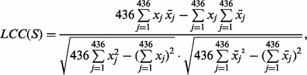where x_j is the mean value of the j-th 2-grams, , in the positive training dataset and x_j is the feature value of the j-th 2-grams with respect to the protein sequence S, defined as x_j = c_j/(len(S) − 1) in which c_j and len(S) are the number of the occurrence of the j-th 2-grams in the sequence S and the length of S, respectively. Note that in our study we selected the 30 features only from the 400 2-grams but not from the 6-letter exchange group, since the latter is derived from PAM (Dayhoff et al., 1978) and has been considered in the scoring matrix features already, as discussed above. However, we need the latter part to calculate the LCC value. Finally, we got 31 PSS features in total.

2.2.4 Annotated features

Following Jones et al. (2008), we extracted 29 features by retrieving several databases, including UniProt KnowledgeBase, SwissProt variant page and COSMIC database. Note that these features include 14 binary categorical features (features 98 through 111 in Supplementary Table S1) annotated in the ‘FT’ (Feature Table, see Supplementary Fig. S1) domain of the UniProt KnowledgeBase, which means if the mutated gene in study is not included in the database, these features are unavailable for the referring mutations. For simplicity, we will next call these 14 features as additional features. This situation largely restricted the applicability of the involved methods, as mentioned above. We extracted these features for comparison, which will be further discussed shortly.

2.3 Feature selection (DX score)

Feature selection is performed in order to remove the most irrelevant and redundant features and ultimately and help improve the performance of learning models. Different methods have been proposed to implement the feature selection. Here we solve this problem based on the DX score as shown above, where the author adopted it to pick out the most relevant 2-gram features (Wang et al., 2001). Intuitively, this DX score bears the capability of assessing a feature’s discrimination power in general case. By the following definition (see Solovyev and Makarova, 1993), the DX score can be considered as a type of signal-noise-ratio:

where m₁ and d₁ (m₀ and d₀, respectively) are the mean value and the standard deviation of the feature in the positive (negative, respectively) training dataset. Intuitively, the larger the DX score, the feature more likely separates the positive from the negative. We further point out that the DX score is equal to the feature score (scaled by a constant) given by the feature selection tool fselect.py of LIBSVM. In addition, the feature selection result obtained by DX score is comparable to the SVM-RFE algorithm, but is superior to the SVM-RFE in computational complexity. The detail concerning these issues is presented in the Supplementary Materials.

2.4 Classification using SVM

SVM algorithm was proposed by Vapnik as an effective learning approach for solving two-class pattern recognition problems (Boser et al., 1992; Cortes and Vapnik, 1995). SVM as a typical supervised machine learning method is attractive because it is not only well founded theoretically but also superior in practical applications. In most of the pattern recognition areas, SVM performs substantially better than that of other machine learning methods, including Neural Network and Decision Tree classifier (You et al., 2010). In this study, we employed two SVM tools LIBSVM (Chang and Lin, 2011) and SVMlight (Joachims, 1999) as classifiers, depending on specific purposes. The updated version of LIBSVM can perform the CV automatically, while SVMlight calculates a continuous value reflecting the probability of each classification, which facilitates the ROC and PR analyses. The precision and recall statistics are computed as: precision = TP/(TP + FP) and recall = TP/(TP + FN). Furthermore, it is straightforward to build a classifier using these two software since all we need to do is to choose a kernel function and to set the related parameters, certainly an input file with standard SVM format is also required. After various trials of different parameters for best performance, we chose the radial basis function with parameter gamma = 0.03 and other parameters remained default for both classifiers.

2.5 CV methods

Machine learning methods are generally evaluated by a statistical technique called CV. In n-fold CV, we first collected a training dataset with equal number of both types (drivers and passengers) and then randomly partitioned the dataset into n subsets of approximately equal size, with each subset still containing an equal number of mutations of both types. Finally, n − 1 such subsets are combined for training the classifier, which is subsequently tested on the withheld data. This procedure is repeated n times with each subset playing the role of the test subset once. The prediction accuracy of n-fold CV is defined as the percentage of missense mutations correctly classified in the test phrase, averaging on n times of tests.

3 RESULTS

3.1 Optimization of the feature space

Preliminarily, we collected 29 492 neutral polymorphisms possessing domain ‘Main gene name’ (to differ from those records simply identified as ‘n.a.’) from the Swiss-Prot website and 4881 cancer-associated missense mutations with explicit mutation profile from the 42nd version of COSMIC database (details in Section 2). By removing polymorphisms whose associated gene overlaps with records in the cancer-associated dataset, we got 23 956 polymorphisms. Using the GeneCards database, we mapped most of the detected polymorphisms to the UniProtKB database and finally extracted all the 126 features for 23 888 polymorphisms and 4193 cancer-associated mutations, respectively. In our configuration, cancer-associated mutations are labeled positive and neutral polymorphisms negative. To relieve the unbalance of the training data, we randomly chose 4193 polymorphisms from the whole 23 888 ones and constructed the training dataset with the two sets of equal size (4193 positive and 4193 negative).

Then we calculated the DX score of each feature of the training data and ranked them from high to low. Following Krishnan et al. (Krishnan and Westhead, 2003), we obtained the final feature space through the steps as follows: set up an empty feature set first, features are then added sequentially (with DX score from high to low) into the basic set to test their impact on the prediction performance, based on 5-fold CV accuracy. This procedure is illustrated in Figure 2, from which it can be seen that the highest accuracy was achieved by adopting the top-ranked 70 features. We also tried several different folds and kernel functions to repeat this procedure and got very similar results (Supplementary Fig. S2). The top-ranked 70 features together with their DX scores are listed in Supplementary Table S2.

Fig. 2.

Performance of 5-fold CV by adding features sequentially. The highest prediction accuracy was achieved using the top-ranked 70 features with 5-fold CV and RBF as kernel function

3.2 Performance of the features in discrimination

Jones et al. (2008) and Parsons et al. (2008) adopted the same 58 predictive features to analyze missense mutations of human pancreatic cancer and glioblastoma multiforme respectively, while Carter et al. (2009) selected 49 from 90 candidate predictive features to perform driver mutation prediction. The two feature sets stand for the hitherto most comprehensive ones in the existing driver mutation identification studies. The latter 49 features largely overlapped with the former 58 ones, of which 41 features can be extracted (underlined ones in Supplementary Table S1). The remaining features predicted by computational algorithms are missed here because of software accessibility issue. However, the extracted 41 features assumedly possess the essential information contained in the 58 ones, since the predicted structural and functional impacts of the residue have already been implicitly included in the biochemical properties of amino acids and the windows-based sequence composition features. In the present study, if there are no special instructions, we compare two feature spaces, one composed of 41 features, which we term ‘previous’, and our enlarged feature space, composed of 70 features with feature selection, which we term ‘proposed’.

A summary of the feature selection result is presented in Table 1, where ‘Hit’ refers to the number of previous features ranking the top 70. It is apparent from Table 1 that the eventual feature set mainly consists of SSM and PSS features that never or seldom used before, whereas only 12 out of the previously used 41 features were selected by the scoring (Fig. 3). This implies many powerful discriminators were neglected in the previous work and on the other hand, the existing could not capture the essential information of a missense and hence cannot serve as effective discriminators.

Table 1.

Summary of the feature selection result

	AARC	SSM	PSS	AF	Total
Proptosed	15	51	31	29	126
Top 70	1	40	21	8	70
Previous	7	5	0	29	41
Hit	0	4	0	8	12

We proposed a total of 126 features belonging to four disjoint groups. 12 out of 41 previously used features ranked within the top 70.

Fig. 3.

DX scores of the top 70 features. Only 12 out of 41 features proposed by Jones et al. ranked within the top 70. Among the 12 features selected by the DX scoring system, 7 are additional features; see Supplementary Table S1. This implies that a large part of the effective features in the existing methods has applicability problem

To evaluate the performance of the selected features in discriminating between driver and passenger mutations, we performed hierarchical clustering analysis to them. For clarity of illustration, we randomly extracted a subset of missense mutations of each type from the original training data to do clustering analysis. Figure 4 [drawn by Cluster 3.0 (de Hoon et al., 2004) with centroid linkage method] shows the effect of hierarchical clustering on 100 neutral polymorphisms plus 100 cancer-associated missense mutations, represented by the above mentioned 70 features. The left patch mainly constitutes cancer-associated mutations while the right patch is dominated by neutral polymorphisms. Apparently, the features which well separate the mutations almost locate in the middle part, and they mainly comprise SSM and protein position-specific features (see Table 1).

Fig. 4.

Hierarchical clustering analysis for a representative subset of mutations of each type. Shown is the clustering result on 200 randomly chosen training samples with equal size for each type. The rows correspond to features and columns represent mutations to be clustered

3.3 Comparison of the prediction performance with others’ work

A 5-fold CV experiment with carefully calibrated parameters was performed on a large set of training data, which contained 4193 polymorphisms versus 4193 cancer-associated missense mutations. Figure 5 shows the comparison of the prediction performance with previous work [referring to the 41 features proposed by Carter et al. (2009), Jones et al. (2008) and Parsons et al. (2008)]. We have an overall 5-fold CV accuracy (Section 2) of up to 83.7%, which is better than or comparable to previous studies, say Kaminker et al. (2007); Krishnan and Westhead (2003); Ng and Henikoff (2001); and Yue and Moult (2006) report overall error rate generally larger than 0.2. Other study which reports higher accuracy than ours has applicability problem in some cases. Specifically, the aforementioned 14 additional features (7 of them were selected into the best 70 features, Table S1), which were proposed by Jones et al. (2008), Parsons et al. (2008) and Carter et al. (2009) individually, may be unavailable for some referred mutations (see Section 2). To investigate the role played by these additional features (14 and 7 features of previous and our proposed feature space respectively) on the classification effect, we performed CV (with same folds and parameter settings) with and without them on the same training set. As expected, we generally got higher prediction accuracy with these additional features than without them. However, our proposed feature space consistently outperformed the previous in both cases (Fig. 5).

Fig. 5.

Comparison of prediction accuracy obtained by previous and our proposed feature space. Shown is the average performance of 5-fold CVs. The terms including and excluding refer to tests performed with and without the additional features, respectively

To gain a test set, we picked out 117 EGFR and 1029 TP53 missense mutations (held out of the training data) which are known as driver mutations for many human cancers from the latest version of COSMIC database (v57). We compared the performance of our method with the previous ones via ROC and PR curves. To do this, we collected 4539 neutral variants from the latest release of the file Humsavar.txt (see Section 2) as passenger mutations. Figure 6 shows the ROC and PR curves calculated for previous and our proposed method on the aforementioned EGFR and TP53 driver mutations and passenger ones. Our method is slightly superior to the previous one on these two sets. In fact, both methods identified almost all the drivers but ours has much higher specificity (true negative rate, see Table 2).

Fig. 6.

ROC and PR curves calculated for previous and our proposed method on (A) 117 EGFR and (B) 1029 TP53 missense mutations, each with 4539 neutral polymorphisms held out of the training set

Table 2.

Number of missense mutations correctly classified by previous and our proposed method

	Neutral	EGFR	TP53	Cosmic2+
Previous	3773 (4539)	117 (117)	1029 (1029)	894 (1113)
Proposed	3888 (4539)	117 (117)	1029 (1029)	940 (1113)

Shown in parentheses are numbers of all mutations used in each test.

However, the relevance of missense mutation of EGFR/TP53 genes to oncogenesis has widely been verified. The possibility that they possess significant biochemical properties relevant to cancer assumedly makes them easy to be identified as drivers. To further assess the performance of our proposed method and previous ones, we test them on an extra mutation set. This extra test dataset consists of 1113 missense mutations still culled from the latest release of COSMIC. They should be absent from the training set and appear in at least two cancer samples (cosmic2+). The collection of passenger mutations was compiled in a similar manner. Figure 7 illustrates the ROC curves calculated for previous and our proposed method on the cosmic2+ driver set and aforementioned passenger set. It can be seen from Figure 7 and Table 2 that previous method missed many driver mutations in this extra set.

Fig. 7.

ROC and PR curves calculated for previous and our proposed method on 1113 missense mutations appearing in at least two cancer samples in COMIC along with 4539 neutral polymorphisms held out of the training set

Finally, we applied the constructed classifier to two published datasets corresponding to human breast and colorectal cancers to test its prediction capability (Sjoblom et al., 2006). The datasets contain 794 and 662 missense mutations of breast and colorectal cancers, respectively, 642 and 502 of which can be covered by both previous and our proposed method. Table 3 lists the number of breast/colorectal mutations classified as drivers by previous and our proposed method, where ‘Consensus’ refers to the number of mutations simultaneously predicted to be drivers by both methods. The number in each parenthesis represents the total number of mutations to be classified for each case. The details of the driver genes predicted by previous and our proposed method are shown in Supplementary Figure S3.

Table 3.

Number of breast/colon mutations classified as drivers by previous and our proposed method

	Breast	Colon
Previous	122 (745)	69 (608)
Proposed	67 (642)	40 (502)
Consensus	18	6

Shown in each parenthesis is the number of all mutations used in each test.

There is a lack of straightforward way to assess which method picked out more actual driver mutations due to the unavailability of definite biological experiments (the original paper identified drivers by a statistical method). Actually, this is a general problem encountered by related researchers, as mentioned in Section 1; see also Gonzalez-Perez and Lopez-Bigas (2011). We hence resorted to published resources on protein sequence and functional annotations to investigate the relevance of these mutations. Concretely, we scrutinized the ontology annotations of each predicted driver gene with respect to its biochemical properties in the UniProtKB database (Wu et al., 2006) by checking a set of keywords appearing in the ‘KW’ domain (red rectangle in Supplementary Fig. S1). These keywords involve biological processes thought to be crucial for cancer progression (Hanahan and Weinberg, 2000; Weinberg, 2006), including ‘apoptosis’, ‘cell cycle’ and ‘signaling pathway’. Intuitively if one gene were annotated with them, it more likely turns out to be a driver. As shown in Figure 8, for both breast and colorectal cancer types, we invariantly got higher percentages of driver genes annotated with at least one of the three keywords.

Fig. 8.

Ontology annotations of driver genes predicted by previous and our proposed method. Shown is the percentage of predicted driver genes (of each cancer type) annotated with one of the three keywords: apoptosis, cell cycle and signaling pathway by the UniProtKB database. The term colon refers to colorectal cancer

On the other hand, our results revealed generally much fewer driver mutations in both cancer types than previous study (10.4% versus 16.4% for breast and 8.0% versus 11.3% for colon, Table 3), which is more consistent with the fact that in most cancer genomes passenger mutations take the bulk (Stratton et al., 2009). Another evidence that supports our results lies in three comment papers (Forrest and Cavet, 2007; Getz et al., 2007; Rubin and Green, 2007), in which the authors re-analyzed the data in Sjoblom et al. (2006) with corrected parameters and obtained reduced number of candidate driver mutations.

4 DISCUSSION

In this work, we dramatically enlarged the existing features used for missense mutation classification, and consequently improved the prediction performance of previous classifiers that discriminate between driver and passenger mutations. Besides incorporating and extending existing features in relation to amino acid properties and binary categorical features extracted from published databases, we for the first time, to our best knowledge, systematically studied all kinds of SSM and investigated their potential power in distinguishing missense mutations. In addition, we are the first to extensively explore the protein sequence patterns instead of structural profiles predicted computationally. This is justified in that protein structure prediction is largely based on sequence alignment with proteins whose structures are already known, hence we rationally expect less information loss by parsing the sequences directly. Indeed, our feature selection scheme confirms the high performance of the SSM and PSS features in separating driver mutations from passenger ones.

The 5-fold CV experiments performed on a large set of training data consistently showed strong prediction capability of our method, both in accuracy and robustness. By applying the trained classifier to several datasets of missense mutations culled from published databases and literature, we obtained more reasonable prediction results than previous studies (by ROC and PR curves as well as functional relevance analysis). Hence, our proposed novel feature extraction scheme is hoped to significantly improve the current work of driver mutation identification.

Another highlight of our work is that the feature extraction scheme depends little on other computational software or databases, which extended the applicability substantially. In principle, given the mutation with associated protein sequence, our system could automatically extract all the features except for the 14 additional ones as mentioned; while if the referred mutation happens to be annotated in the UniProtKB database, then all the 126 features can be extracted without depending on any other software or databases (although our tool only chooses the top-ranked 70 ones for default). The reason that some data in the classifying part cannot be covered lies in the fact that the original paper did not provide the corresponding protein sequences but only a gene name/ID instead. In this case, we have to map it to related databases to extract its protein sequence first. At this step, if one data use a very uncommon gene name/ID then we cannot map it to the records in UniProtKB, even under the help of GeneCards. Another reason of miss-covering is we discarded the mutations at the beginning and end of a sequence in that windows-based amino acid residue sequence composition features could not handle them. In practice, such kind of mutations with missing values can be treated as in Carter et al. (2009).

Of note, only one of the 15 AARC features ranked within the top 70, namely the number of hydrogen atoms of one amino acid. This is probably because most information of the amino acid has been already contained in the SSM features, for example, the 42nd feature incorporates biochemical and biophysical properties of amino acids to construct the WAC matrix (Wei et al., 1997). A large part of SSM and PSS features were selected by the DX scoring scheme, namely, 40 out of 51 and 21 out of 31 for the former and latter, respectively. What is attractive is one of the sequence specific features LCC ranks very top—it gets the fourth highest DX score. This again confirms that PSS features play a very significant role on discrimination.

Our proposed method outperforms previous ones, whether or not including the additional features (Fig. 5). However, both methods got higher CV accuracy when including the additional categorical features (features 98 through 111, Supplementary Table S1). This clearly demonstrates their superior distinguishing capability, and the superiority was further boosted by the facts that half of this part was selected (7 out of 14) by DX score and two features of them ranked the top 2. This is not surprising by checking the description in Supplementary Table S2, namely, they are annotated in the ‘FT’ domain (Supplementary Fig. S1) as ‘MUTAGEN’ and ‘MOD_RES’ which refer to mutagenic sites and modified residues, respectively. Intuitively, a mutation with such features is more likely to be a deleterious substitution or a disease-causing mutation. Considering the importance of this part of features, we suggest that for a newly submitted mutation for which the additional features are unavailable, one can extract the remaining 63 features and leave the 7 specials (only 7 of them were selected into the final feature set) empty, since most of the existing software can handle the data with missing features, for example, the SVMlight (Joachims, 1999).

Although our work rectifies several shortcomings of the existing studies, further improvements are both needful and possible. Particularly, the persistent update of related database cited in this study is expected to improve the performance of our proposed method. For example, new scoring matrix may expand the feature space and make the classifier more effective; the increasing integrity of GeneCards database could improve the coverage of our system, i.e. more mutations can be predicted in an automatic sense. On the other hand, the number and signature of driver mutations vary between cancer types. Therefore, classifier trained with data of same cancer type may be more effective to classify mutations of that cancer. To make the training dataset self-adaptive to a particular classification problem will appear in our future work.

REFERENCES

- Boser BE, et al. A training algorithm for optimal margin classifiers. Proceedings of the Fifth Annual Workshop on Computational Learning Theory; ACM, Pittsburgh, Pennsylvania. 1992. pp. 144–152. [Google Scholar]
- Carter H, et al. Cancer-specific high-throughput annotation of somatic mutations: computational prediction of driver missense mutations. Cancer Res. 2009;69:6660–6667. doi: 10.1158/0008-5472.CAN-09-1133. [DOI] [PMC free article] [PubMed] [Google Scholar]
- Chang C-C, Lin C-J. LIBSVM: a library for support vector machines. ACM Trans. Intelligent Syst. Technol. 2011;2:27:21–27:27. [Google Scholar]
- Cortes C, Vapnik V. Support-vector networks. Machine Learn. 1995;20:273–297. [Google Scholar]
- Dayhoff MO, et al. A model of evolutionary change in proteins. Atlas Prot. Seq. Struc. 1978;5:345–352. [Google Scholar]
- de Hoon MJ, et al. Open source clustering software. Bioinformatics. 2004;20:1453–1454. doi: 10.1093/bioinformatics/bth078. [DOI] [PubMed] [Google Scholar]
- Forrest WF, Cavet G. Comment on ‘The consensus coding sequences of human breast and colorectal cancers’. Science. 2007;317:1500. doi: 10.1126/science.1138179. author reply 1500. [DOI] [PubMed] [Google Scholar]
- Getz G, et al. Comment on ‘The consensus coding sequences of human breast and colorectal cancers’. Science. 2007;317:1500. doi: 10.1126/science.1138764. [DOI] [PubMed] [Google Scholar]
- Gonzalez-Perez A, Lopez-Bigas N. Improving the assessment of the outcome of nonsynonymous SNVs with a consensus deleteriousness score, Condel. Am. J. Hum. Genet. 2011;88:440–449. doi: 10.1016/j.ajhg.2011.03.004. [DOI] [PMC free article] [PubMed] [Google Scholar]
- Grantham R. Amino acid difference formula to help explain protein evolution. Science. 1974;185:862–864. doi: 10.1126/science.185.4154.862. [DOI] [PubMed] [Google Scholar]
- Greenman C, et al. Statistical analysis of pathogenicity of somatic mutations in cancer. Genetics. 2006;173:2187–2198. doi: 10.1534/genetics.105.044677. [DOI] [PMC free article] [PubMed] [Google Scholar]
- Hanahan D, Weinberg RA. The hallmarks of cancer. Cell. 2000;100:57–70. doi: 10.1016/s0092-8674(00)81683-9. [DOI] [PubMed] [Google Scholar]
- Henikoff S, Henikoff JG. Amino acid substitution matrices from protein blocks. Proc. Natl Acad. Sci. USA. 1992;89:10915–10919. doi: 10.1073/pnas.89.22.10915. [DOI] [PMC free article] [PubMed] [Google Scholar]
- Joachims T. Advances in Kernel Methods. Cambridge, MA, USA: MIT Press; 1999. Making large-scale SVM learning practical; pp. 169–184. [Google Scholar]
- Jones S, et al. Core signaling pathways in human pancreatic cancers revealed by global genomic analyses. Science. 2008;321:1801–1806. doi: 10.1126/science.1164368. [DOI] [PMC free article] [PubMed] [Google Scholar]
- Kaminker JS, et al. Distinguishing cancer-associated missense mutations from common polymorphisms. Cancer Res. 2007;67:465–473. doi: 10.1158/0008-5472.CAN-06-1736. [DOI] [PubMed] [Google Scholar]
- Kawashima S, et al. AAindex: amino acid index database, progress report 2008. Nucleic Acids Res. 2008;36:D202–D205. doi: 10.1093/nar/gkm998. [DOI] [PMC free article] [PubMed] [Google Scholar]
- Krawczak M, et al. Human gene mutation database—a biomedical information and research resource. Hum. Mutat. 2000;15:45–51. doi: 10.1002/(SICI)1098-1004(200001)15:1<45::AID-HUMU10>3.0.CO;2-T. [DOI] [PubMed] [Google Scholar]
- Krishnan VG, Westhead DR. A comparative study of machine-learning methods to predict the effects of single nucleotide polymorphisms on protein function. Bioinformatics. 2003;19:2199–2209. doi: 10.1093/bioinformatics/btg297. [DOI] [PubMed] [Google Scholar]
- Lancet D, et al. GeneCards tools for combinatorial annotation and dissemination of human genome information. GIACS Conference on Data in Complex Systems; 2008. Palermo, Italy. [Google Scholar]
- Ng PC, Henikoff S. Predicting deleterious amino acid substitutions. Genome Res. 2001;11:863–874. doi: 10.1101/gr.176601. [DOI] [PMC free article] [PubMed] [Google Scholar]
- Ng PC, Henikoff S. Accounting for human polymorphisms predicted to affect protein function. Genome Res. 2002;12:436–446. doi: 10.1101/gr.212802. [DOI] [PMC free article] [PubMed] [Google Scholar]
- Parmigiani G, et al. Johns Hopkins University, Dept. of Biostatistics Working Papers. 2007. Statistical methods for the analysis of cancer genome sequencing data. Working Paper 126. [Google Scholar]
- Parsons DW, et al. An integrated genomic analysis of human glioblastoma multiforme. Science. 2008;321:1807–1812. doi: 10.1126/science.1164382. [DOI] [PMC free article] [PubMed] [Google Scholar]
- Rubin AF, Green P. Comment on ‘The consensus coding sequences of human breast and colorectal cancers’. Science. 2007;317:1500c. doi: 10.1126/science.1138956. [DOI] [PubMed] [Google Scholar]
- Sjoblom T, et al. The consensus coding sequences of human breast and colorectal cancers. Science. 2006;314:268–274. doi: 10.1126/science.1133427. [DOI] [PubMed] [Google Scholar]
- Solovyev VV, Makarova KS. A novel method of protein sequence classification based on oligopeptide frequency analysis and its application to search for functional sites and to domain localization. Comput. Appl. Biosci. 1993;9:17–24. doi: 10.1093/bioinformatics/9.1.17. [DOI] [PubMed] [Google Scholar]
- Stratton MR, et al. The cancer genome. Nature. 2009;458:719–724. doi: 10.1038/nature07943. [DOI] [PMC free article] [PubMed] [Google Scholar]
- Sunyaev S, et al. Prediction of deleterious human alleles. Hum. Mol. Genet. 2001;10:591–597. doi: 10.1093/hmg/10.6.591. [DOI] [PubMed] [Google Scholar]
- Wang JTL, et al. New techniques for extracting features from protein sequences. IBM Syst. J. 2001;40:426–441. [Google Scholar]
- Wei LP, et al. Using the radial distributions of physical features to compare amino acid environments and align amino acid sequences. Pacific Symposium on Biocomputing. 1997;97:465–476. [PubMed] [Google Scholar]
- Weinberg RA. Cancer biology and therapy: the road ahead. Cancer Biol. Ther. 2002;1:3. doi: 10.4161/cbt.1.1.28. [DOI] [PubMed] [Google Scholar]
- Weinberg RA. New York: Garland Science; 2006. The biology of cancer; p. 864. [Google Scholar]
- Weir B, et al. Somatic alterations in the human cancer genome. Cancer Cell. 2004;6:433–438. doi: 10.1016/j.ccr.2004.11.004. [DOI] [PubMed] [Google Scholar]
- Wood LD, et al. The genomic landscapes of human breast and colorectal cancers. Science. 2007;318:1108–1113. doi: 10.1126/science.1145720. [DOI] [PubMed] [Google Scholar]
- Wu C, et al. Protein classification artificial neural system. Protein Sci. 1992;1:667–677. doi: 10.1002/pro.5560010512. [DOI] [PMC free article] [PubMed] [Google Scholar]
- Wu CH, et al. The Universal Protein Resource (UniProt): an expanding universe of protein information. Nucleic Acids Res. 2006;34:D187–D191. doi: 10.1093/nar/gkj161. [DOI] [PMC free article] [PubMed] [Google Scholar]
- Wu CH, et al. Neural networks for full-scale protein sequence classification: sequence encoding with singular value decomposition. Machine Learn. 1995;21:177–193. [Google Scholar]
- You ZH, et al. A semi-supervised learning approach to predict synthetic genetic interactions by combining functional and topological properties of functional gene network. BMC Bioinformatics. 2010;11:343. doi: 10.1186/1471-2105-11-343. [DOI] [PMC free article] [PubMed] [Google Scholar]
- Yue P, Moult J. Identification and analysis of deleterious human SNPs. J. Mol. Biol. 2006;356:1263–1274. doi: 10.1016/j.jmb.2005.12.025. [DOI] [PubMed] [Google Scholar]
Associated Data
This section collects any data citations, data availability statements, or supplementary materials included in this article.