Reducing grid-dependence in finite-difference Poisson-Boltzmann calculations

Abstract

Grid dependence in numerical reaction field energies and solvation forces is a well-known limitation in the finite-difference Poisson-Boltzmann methods. In this study we have investigated several numerical strategies to overcome the limitation. Specifically, we have included trimer arc dots during analytical molecular surface generation to improve the convergence of numerical reaction field energies and solvation forces. We have also utilized the level set function to trace the molecular surface implicitly to simplify the numerical mapping of the grid-independent solvent excluded surface. We have further explored to combine the weighted harmonic averaging of boundary dielectrics with a charge-based approach to improve the convergence and stability of numerical reaction field energies and solvation forces. Our test data show that the convergence and stability in both numerical energies and forces can be improved significantly when the combined strategy is applied to either the Poisson equation or the full Poisson-Boltzmann equation.

Introduction

Biomolecules are highly complex molecular machines with thousands to millions of atoms. What further complicates the picture is the need to realistically treat the interactions between biomolecules and their surrounding water molecules that are ubiquitous and paramount important for their structures, dynamics, and functions. An efficient molecular dynamics simulation in a realistic aqueous environment is still one of the few remaining challenges in computational chemistry.^1-14

Since most particles in molecular dynamics are to represent water molecules solvating the target biomolecules, treating these water molecules implicitly allows the simulation efficiency to be increased greatly. Indeed, implicit solvation treatments, or implicit solvents, offer a unique opportunity for more efficient simulations without the loss of atomic-level resolution for biomolecules. The simplified implicit solvation treatments propose to model water molecules and all dissolved ions as a structureless and continuous medium. In contrast, biomolecules, i.e. the solutes, are still represented in atomic detail. One of the most successful implicit solvents, the Poisson-Boltzmann (PB) implicit solvent,¹⁵ has become a gold standard in implicit solvation treatments of biomolecules after years of basic research and development.

Adaptation of the PB solvents to molecular simulations requires a numerical solution of the 3-D partial differential equation, which has been a bottleneck, largely limiting their application to calculations with static structures only. The difficulty lies in the numerical procedure that involves discretization of the partial differential equation into a system of linear or nonlinear equations that tends to be rather large: it is not uncommon to have tens of millions of unknowns in biochemical applications. In addition, the setup of the system before the numerical solution and post-processing to obtain energies and forces are both nontrivial. Three major discretization methods are widely used in biomolecular applications. The most commonly used approach is the finite-difference method.^16-31 In this method, the physical properties of the solution such as atomic charges and dielectric constants are mapped onto a rectangular grid, and a discrete approximation to the governing partial differential equation is produced. The second approach is the finite-element method,^32-37 which approximates the potential by a superposition of a set of basis functions. A linear or nonlinear system for the coefficients produced by the weak formulation has to be solved. The third approach is the boundary-element method.^38-51 In the boundary-element method, the Poisson or Poisson-Boltzmann equation is solved for either the induced surface charge38-40,42,44,45,48,51 or the normal component of the electric displacement^{41,43,46,47,49,50} on the dielectric boundary between the solute and the solvent.

A crucial component of all implicit solvent models within the PB framework is the dielectric model, i.e. the dielectric constant distribution of a given solution system. Typically, a solution system is divided into the low dielectric interior and the high dielectric exterior by a molecular surface. That is to say that the molecular surface is used as the dielectric interface between the two piece-wise dielectric constants. The solvent excluded surface (SES)^52-54 is the most used surface definition.^25,27 Indeed, recent comparative analyses of PB-based solvent models and TIP3P solvent models show that the SES definition is reasonable in calculation of reaction field energies and electrostatic potentials of mean force of hydrogen-bonded and salt-bridged dimers with respect to the TIP3P explicit solvent.^55-57 Given the complexity of the SES, one possible approach in adapting the SES in numerical solutions is to build the molecular surface analytically and then to map it onto a grid,^58-60 though analytical procedures can be time consuming. Rocchia et al. subsequently simplified the algorithm to facilitate the mapping of the SES to the grid.²⁷ The van der Waals (VDW) surface, or the hard sphere surface, represents the low-dielectric molecular interior as a union of atomic van der Waals spheres. This is a very efficient algorithm, though there exist many nonphysical high (solvent) dielectric pockets inside the solute interior when the VDW definition is used. Considering the limitation, the modified VDW definition was proposed. The basic idea of the modified VDW definition is to use the solvent accessible surface (SAS) definition for fully buried atoms and the VDW definition for fully exposed atoms.⁶¹ However, the method is difficult to be optimized to reproduce the more physical SES definition. The density approaches have recently been developed and can be used for numerical PB solutions. Either a Gaussian-like function or a smoothed step function has been explored in previous developments.^62,63 Recently it has been shown that if the functional form is allowed to change, the density function can be explicitly optimized to reproduce the classical SES definition at least for certain “small” solvent probe radii, though this cannot be generalized to arbitrary probe radius values.⁶⁴ In this type of approaches, a distance-dependent density/volume exclusion function is used to define each atomic volume or the dielectric constant directly. This is in contrast to the hard-sphere definition of atomic volume as in the VDW or the SES definition. Therefore, all surface cusps are removed by the use of smooth density functions.^62,63

Once a molecular surface definition is chosen, it can be used to specify the dielectric constant distribution in space. Due to the finite-difference discretization of space, the dielectric constant distribution depends on the location and orientation of the finite-difference grid with respect to the molecule of interest. In general, different locations/orientations lead to different dielectric distributions, which in the end lead to different numerical energies and forces. This is termed as numerical uncertainty or instability below. In addition, different grid spacings resolve the molecular surface differently, and apparently a finer grid resolves the molecular surface better. This leads to the second difficult problem that is how to reduce the grid dependence in the numerical energies and forces when a “not-a-too-fine” grid spacing (i.e. ½ Å) has to be used in practical applications. Of course, discretization of atomic point charges is yet another source of numerical uncertainty and grid dependence in the finite-difference solutions. Several general strategies have been proposed in the past to reduce these numerical issues. The first strategy intends to “smooth” the sharp transition of dielectrics between the solute and solvent via the weighted harmonic averaging method.^65,66 Of course, it is also possible to change the underlining physical model, i.e. the sharp transition at the solute/solvent interface can be changed to a distance-dependent transition as in the density function approach, though this amounts to the development of a different force field and is beyond the scope of this study.⁶² Interestingly, the weighted harmonic averaging method was also proposed to combine with the distance-dependent dielectric model for better numerical behavior.⁶⁷ The second strategy focuses on the treatment of point charges. In this method, the point charges are spread to the nearest grid points as in the trilinear interpolation method.⁶⁸ Of course, it can also be used along with the dielectric smoothing method discussed above.⁶⁸ The third strategy utilizes the grid-independent molecular surface to compute numerical energies via the charge-based method.²⁷ The basic concept has also been extended to the computation of solvation forces.⁶⁹

Based on these pioneering efforts for more reliable numerical solutions of the PB equation for biomolecules, we intend to overcome the numerical difficulty associated with the solvent excluded surface definition in the following aspects: (1) simplification of the numerical procedure and reduction in computer memory usage when mapping the grid-independent surface definition onto the finite-difference grid and (2) exploration of strategies to minimize the dependence of numerical energies and solvation forces upon the grid spacing used in the finite-difference Poisson-Boltzmann methods.

Methods

Assignment of dielectric constant nearby solute interface

In biomolecular calculations the dielectric distribution often adopts a piece-wise constant model. In such a model, the dielectric constant at the midpoint of a grid edge should be equal to the dielectric constant in the region where the two neighboring grid points reside. However, when the two neighboring grid points belong to different dielectric regions, the dielectric constant is nontrivial to assign because the dielectric constant is discontinuous across the interface. Denote the dielectric constants inside and outside as ε_in and ε_out, respectively. The simplest treatment is to set the dielectric constant as ε_in if the midpoint of the grid edge is in the solute or ε_out otherwise, as in the Delphi program.²⁷ We term this treatment as the non-harmonic averaging (NHA) method. In this study, we further revise the NHA method as follows

$$\epsilon =\{\begin{array}{cc}{\epsilon }_{in}\hfill & ifa>0.5\hfill \\ {\epsilon }_{out}\hfill & otherwise\hfill \end{array}\phantom{\}},$$ (1)

where a is the fraction of a grid edge inside. This procedure gives the same dielectric assignment as the method adopted in the Delphi program that only considers grid edge midpoints. However, it is different from the Delphi program when the interface intersects the same grid edge twice or more. The revised method is, arguably, more consistent with the concept of the finite-difference discretization but it is apparently time-consuming. This revision is introduced to compare NHA with other methods to be discussed below.

An alternative treatment is the use of harmonic averaging (HA) of the two dielectric constants at the neighboring grid points of a grid edge that intersects the molecular surface.^65,66 In the simple harmonic averaging (SHA) method, the dielectric constant is assigned as

$$\epsilon =\frac{2}{\frac{1}{{\epsilon }_{in}}+\frac{1}{{\epsilon }_{out}}}.$$ (2)

In the weighted harmonic averaging (WHA) method, the dielectric constant is assigned as

$$\epsilon =\frac{1}{\frac{a}{{\epsilon }_{in}}+\frac{1-a}{{\epsilon }_{out}}},$$ (3)

where a, the fraction of the grid edge inside, is also used in eqn (1). It should be pointed out that NHA gives sharp transition in dielectric constant across the interface while WHA or SHA offers one more grid point for a smoother change in the dielectric constant across the interface. Furthermore, WHA guarantees the flux conservation in the three orthogonal directions at the intersection points of grid edges and the analytical interface.

When using any of these treatments, we do not need to generate the molecular surface explicitly. In SHA, grid points need to be labeled inside or outside only. In WHA and NHA, a more elaborate grid point labeling scheme is needed to calculate the intersection points of grid edges and the molecular surface.

Overview of the algorithm

As mentioned above, WHA or NHA requires the computation of fractional grid edges. Our algorithm to compute the fractional grid edges consists of three steps:

1. Determination of solvent accessible arcs. The arcs are numerically represented as dots that are centers of solvent accessible probes tangential to at least two atoms simultaneously. This list of dots and the list of atoms are used to label the grid points nearby the molecular surface.

2. Grid point labeling. The grid points nearby the molecular surface are labeled as inside or outside. Furthermore, an arc dot or an atom is assigned to a grid point according to its position with respect to the molecular surface. These labels are used to compute the fractional grid edges.

3. Computation of the fractional grid edges. After the grid points are labeled, the fractional grid edges can be computed arithmetically or geometrically.

The detail of these three steps is described below. Then the dielectric constants nearby the molecular surface can be assigned by NHA or WHA method according to eqn (1) or (3), respectively.

Determination of solvent accessible arcs

Solvent accessible arcs were first used to generate the molecular surface in Connolly’s work, instead of evenly-distributed surface dots.⁵⁴ Using these solvent accessible arcs, You et al suggested an analytical algorithm to differentiate the grid points inside or outside of the molecular surface.⁶⁰ Rocchia et al. subsequently simplified the algorithm to use a set of dots to represent the solvent accessible arcs to facilitate the reentry surface’s mapping to the finite-difference grid.²⁷

In this study, we follow the basic idea as outlined by You et al.⁶⁰ and Rocchia et al.²⁷ Specifically, a numerical representation of the solvent accessible arcs was used to map the reentry surface to the finite-difference grid. A parameter termed arcres (in Å) was introduced to represent the discretization resolution of the solvent accessible arcs. The solvent accessible arc dots were obtained by a “successive pruning” method by exploiting the existing data structure in the force field module of the Amber package. Specifically we utilized the bond/angle lists, the torsion angle lists, and the nonbonded lists to successively prune the candidate dots that were buried in the SAS of neighboring atoms.

Another feature of our algorithm of constructing the solvent accessible arcs is that we intentionally added the trimer arc dots, which are the centers of the probes that are in contact with three atoms. The merit of this extra effort can be appreciated in the following way. With the same resolution of arc dots, the solvation energies and forces are both more accurate with the trimer arc dots included, or with the same requirement of accuracy level, the presence of trimer arc dots can reduce the necessary resolution of arc dots so as to save the memory allocation (the memory required at this step is probably more than that required by the PB solver if a coarse grid spacing, for example 1/2 Å, is used).

Once the solvent accessible arc dots are generated, they are used in the following grid point labeling procedure and the intersection calculation procedure.

Grid point labeling

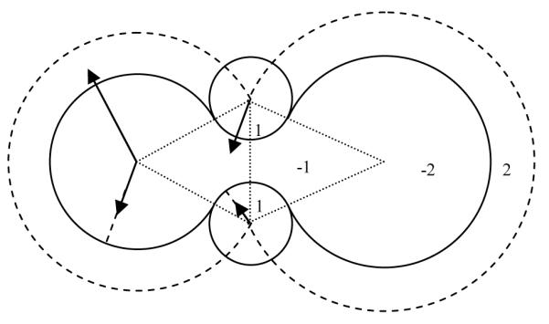
Different from Rocchia et al.,²⁷ our algorithm not only labels grid points inside or outside, but also records additional information to calculate the intersection points to utilize the NHA or WHA method. The algorithm is illustrated in Figure 1 and can be summarized in the following pseudo code:

1. Initialize all grid points as “1”, i.e. in the solvent region.

2. Label all grid points within the extended van der Waals volume as “2”. For each labeled grid point, its signed distances to all the atoms’ van der Waals surface are calculated. The atom with the smallest distance is recorded as the corresponding “owner” of the labeled grid point.

3. Label all grid points within the van der Waals volume as “-2”. The “owner” of a labeled grid point is determined as follows. When the projection point of the grid point on the extended van der Waals sphere of an atom is not in the extended van der Waals spheres of any other atoms, the atom is the corresponding “owner”.

4. Label all grid points within the reentry cones^* of all pairs of neighboring atoms as “-1”.

5. Label all “-1” grid points within the solvent probe spheres at all arc dots as “1”. For each grid labeled as “-1” or “1”, its corresponding “owner” is updated as the closest solvent probe.

Figure 1.

Grid point labeling scheme in the numerical molecular surface procedure.

After the grid point labeling process, grid points with positive labels are in the solvent region and grid points with negative labels are in the solute region. We will present an analysis below on how dense the arc points should be to achieve converged numerical reaction field energies.

It should also be noted that only the “owners” of the grid points nearby the dielectric interface will be used in the computation of the fractional grid edges as described below. Thus the labeling algorithm documented here is only meant to guarantee that these “owners” are assigned correctly.

Computation of fractional grid edges

Given the information provided in the grid point labeling algorithm, there may be different strategies to compute the intersection points of the molecular surface and grid edges. A straightforward method would be a brute-force analytical approach via geometric information recorded in the grid point labeling algorithm. This approach is termed the geometric approach and is discussed in detail in the Supplementary Material. Here we explore a more straightforward algorithm via the level set method.^70,71 This algorithm relies on algebraic manipulations of the level set function, so it is termed the algebraic approach.

In the level set method a scalar function, the level set function, is used to represent the surface implicitly. Here we define the level set function as the following:

$$d=\{\begin{array}{cc}{d}_{g-c}-R_{vdw}\hfill & \text{if labeled as 2 or -2}\hfill \\ -d_{g-c}+R_{prod}\hfill & \text{if labeled as 1 or -1}\hfill \end{array}\phantom{\}}$$ (4)

where d_g–c is the distance between the grid point and the corresponding owner center, R_vdw is the atomic van der Waals radius, and R_prob is the probe radius. Note that the definition in eqn (4) has incorporated the sign notation that grid points on the solvent side have positive values and grid points on the solute side have negative values. In doing so the SES is located where the level set function is zero (d=0), i.e. the zero level set. This is consistent with the original definition of the SES.⁵²

With these preparations, we are ready to compute the intersection point of a boundary grid edge and the molecular surface as follows. Without loss of generality, suppose that this is an x-edge flanked by two grid points (x₁, y₁, z₁) and (x₁ + h, y₁, z₁), where h is the grid spacing. The level set function values are d₁ and d₂, respectively. Apparently, we have d₁ × d₂ < 0 since the sign of the level set function defined by eqn (4) and changes when crossing the molecular surface, and the intersection point is between (x₁, y₁, z₁) and (x₁ + h, y₁, z₁). Next we choose a third grid point, (x₁ + 2h, y₁, z₁). Given the three grid points and corresponding level set functions as d₁ , d₂ , d₃ , respectively, a quadratic function d = a₂x² + a₁x + a₀ can be determined to pass through three points (x₁, d₁), (x₁ + h, d₂), and (x₁ + 2h, d₃). Thus, the intersection point is simply the root of the quadratic equation a₂x² + a₁x + a₀ = 0 within [x₁,x₁+h].

Although the algebraic method proposed here is in principle different from a brute-force utilization of the molecular surface in the geometric algorithm to find the intersection points, it has been shown that the error in the calculated intersection point scales as O(h²) when the level set method is used.^70,71

It should be pointed out that the level set method was used to compute the molecular surface by Can et al.⁷² Their aim is to generate and visualize a molecular surface efficiently, so they calculate the level set function with the error in the order of grid spacing h. By contrast our method calculates the level set function analytically to guarantee the accuracy error in the calculated intersection point scales as O(h²).

Computation of reaction field energy

To compute the reaction field energy, the field-based method is often used, i.e., the reaction field energy is calculated as

$$\Delta G_{rf}=\frac{1}{2}\sum _i^{N_{atom}}{q}_i{\varphi }_i^{RF},$$ (5)

where q_i is the charge of atom i and ${\varphi }_i^{RF}$ is the reaction field potential at the position of atom i, which can be calculated from the grid potential by the tri-linear interpolation method. Direct computation of the reaction field potential is made possible by the so-called charge singularity free formulation of the Poisson-Boltzmann equation.³¹ It has been pointed out that the reaction field energy may converge better when the so-called charge-based method is used.²⁷ In this method, $q_j^{pol}$ , the polarization charge at boundary grid point j, is first calculated according to the Gauss’s law. Then all polarization charges are projected onto the solvent/solute interface as described in Figure 2. Finally the reaction field energy is calculated as

$$\Delta G_{rf}=\frac{1}{2}\sum _i^{N_{atom}}\sum _j^{N_{bnd}}\frac{q_i{q}_j^{pol}}{r_{ij}}$$ (6)

Where N_bnd is the number of polarization charges and r_ij is the distance between atom i and projected polarization charge j.

Figure 2.

Projection procedures of boundary grid points. A “±2” point is projected onto the nearest atom sphere and a “±1” point is projected onto the nearest probe sphere. Note that surface polarizable charges are only located on boundary grid points with non-uniform dielectric constants on its six neighboring grid edges.

Computation of electrostatic solvation forces

It is well known that the electrostatic force density (g) can be derived through the divergence of the Maxwell stress tensor (P) as^69,73

$$\begin{array}{cc}\hfill \mathbf{g}=\nabla \cdot P=& \frac{\partial }{\partial x}(\mathit{i}\cdot P)+\frac{\partial }{\partial y}(\mathit{j}\cdot P)+\frac{\partial }{\partial z}(\mathit{k}\cdot P)\hfill \\ \hfill & ={\rho }^f\mathbf{E}-\frac{1}{8\pi }{E}^2\nabla \epsilon -\Delta \Pi \nabla \lambda ,\hfill \end{array}$$ (7)

where is the fixed charge desnity, E is the electric field, ε is the dielectric constant, and ΔΠ is the excess osmotic pressure, λ is the Stern layer defined so that it is 1 in regions accessible to the mobile ions and 0 elsewhere. This is consistent with the formulation of Gilson et al.⁷⁴ An important point is that eqn (7) requires a differentiable dielectric constant distribution.

Eqn (7) shows that there are three components in the total electrostatic forces: (1) the Coulombic and reaction field forces (g_QEF) acting on the atomic charges, ρ^f E; (2) the dielectric boundary forces (g_DBF), or pressure acting on the dielectric boundary, $-\frac{1}{8\pi }{E}^2\nabla \epsilon$; and (3) the ionic boundary forces, or pressure on the ionic boundary. Since the Coulombic forces can be computed analytically by a pairwise summation of Coulombic interactions among atomic charges, only the rest of the force components were computed numerically.

Similar to the treatment of the reaction field energy, dielectric polarization charges can be used to improve the convergence of reaction field forces with respect to the grid spacing. Specifically, the reaction field forces were calculated by the pairwise summation of the Coulombic interactions between polarizarion charges and atomic charges.²⁷ Briefly, it has been shown that the dielectric boundary forces can be recast into the following form,⁶⁹

$${\mathbf{g}}_{DBF}=g_{DBF}\widehat{\mathbf{n}}=-\frac{1}{8\pi }{E}^2\nabla \epsilon =\frac{1}{2}{\rho }^{pol}\frac{{\mid \mathbf{D}\mid }^2}{D_n}\widehat{\mathbf{n}},$$ (8)

where ρ^pol is the polarization charge density at the dielectric boundary, D = εE , and D_n = εE_n. Eqn (8) does not require a differentiable dielectric constant distribution and makes it explicit that the direction of g_DBF follows the gradient of the dielectric constant, i.e. the normal direction of the surface (n̂).

Due to the fact that the SES is not differentiable, the dielectric boundary force elements are distributed to nearby atoms in an ad hoc manner as follows. For the contact portion of the SES, the surface force elements are distributed to the closest atom sphere. For the reentry portion of the SES, the dielectric boundary force elements are distributed to the two or three nearest atom spheres (if trimer arc dots are present) by the singular value decomposition method (SVD). ⁶⁹

Finally the ionic boundary forces are ~O(10⁻²) smaller than the reaction field forces and dielectric boundary forces in water⁷⁴ so that we only focus on the reaction field forces and dielectric boundary forces in the performance analyses of the dielectric treatments below. In addition, their performance is more closely related to how the Stern layer is defined, which is beyond the scope of this development.

Other computational details

The dielectric constant of the solvent was set to 80, i.e. for water, while that of the solute was set to 1. Both WHA and SHA were analyzed and compared with NHA. The numerical surface algorithm was validated with a solvent probe radius of 1.4 Å. The modified Bondi radius set^75,76 was tested. The ion concentration was set to zero. No electrostatic focusing was used. The finite-difference grid dimension was set to be 2.5 times of the dimension of a solute. The convergence criterion was set to be 10⁻⁶ for the finite-difference solver. All other parameters are either explicitly analyzed or set to be default as in the PBSA program of AMBER 10.^26,61,75,76 To analyze the numerical uncertainty of different methods, a total of 96 different finite-difference grid origins and orientations were used to sample the relative locations of the finite-difference grid with respect to the molecular surface and charge distribution. All the reaction field energies were computed with the charge-view method unless otherwise stated.

Two groups of molecules are studied in this work. The first group includes a hydrogen-bonding base pair GC and a small alanine-based peptide (ALA6) forming an α helix.⁵⁶ These molecules were built in the XLEAP program of AMBER10. The second group was taken from the Amber benchmark suite includes a diversified test set of 579 peptides and proteins.^75,76

Results and Discussion

Abrupt two dielectrics treatment: Consistency between PBSA and Delphi programs

Our numerical mapping algorithm of the SES onto the finite-difference grid certainly resembles the mapping algorithm implemented in the Delphi program. Both programs intend to use the atomic positions and a numerical representation of solvent accessible arcs to map the SES onto the finite-difference grid. Since Delphi uses the NHA method, the dielectric map from the Delphi program should be very similar to that from the PBSA program with the NHA method. However, difference does exist between the two programs: the grid labeling procedure in PBSA focuses on grid points while the procedure in Delphi focuses on grid edge midpoints. This leads to different handling of certain grid edges nearby the molecular surface. For example, if a grid edge is flanked by two interior grid points, PBSA will treat the edge as solute interior. In contrast Delphi would treat the grid edge as interior only when the edge midpoint is also interior. Otherwise, the grid edge is assigned as exterior.

Nevertheless, such boundary grid edges are only a very small fraction of boundary grid edges when (1) the grid spacing is small (i.e. ½ Å) with respect to atom and probe radii and (2) the SES definition is used. Indeed, we calculated the reaction field free energies of 579 biomolecules by PBSA and Delphi and plotted their correlation in Figure 3. The correlation plot shows a very high correlation between the two different algorithms. The Pearson correlation coefficient between the two sets of data is 1.0000, the linear regression slope is 0.9991 (with a fixed offset of zero), and the RMS relative deviation is 0.0012 between the two sets of data. Furthermore, the difference between the two programs also reduces with decreasing grid spacings.

Figure 3.

Top: correlation of reaction field energies by PBSA and Delphi for the 579 biomolecules in the Amber training set. The Pearson correlation coefficient is 1.0000 and the linear regression slope is 0.9991 (with zero offset). Bottom: absolute differences (D_ΔG) between calculated reaction field energies by two programs versus calculated reaction field energies by Delphi. Here both PBSA and Delphi uses the NHA method for the dielectric constant assignment on the molecular surface.

Harmonic averaging dielectrics treatment: Consistency between algebraic and geometric methods

As discussed in the method section, our proposed algebraic method utilizes the concept of the level set function to trace the molecular surface implicitly. Thus the intersection points of the molecular surface and the grid edges are computed via the solution of an algebraic equation within the framework of the level set function. This is clearly different from traditional geometry-based methods where we have to compute the intersection points based on the geometric relations between relevant van der Waals spheres and solvent probe spheres that are located on the solvent accessible arcs.

Here we first demonstrate their high-level consistency in the diversified test set of 579 biomolecules used above. Figure 4 plots the correlation of reaction field energies for these molecules with the algebraic and geometric surfaces, respectively. Overall, the two kinds of surfaces agree excellently, with a linear regression slope of 1.0004 (the offset is fixed at zero) and the Pearson correlation coefficient of 1.0000.

Figure 4.

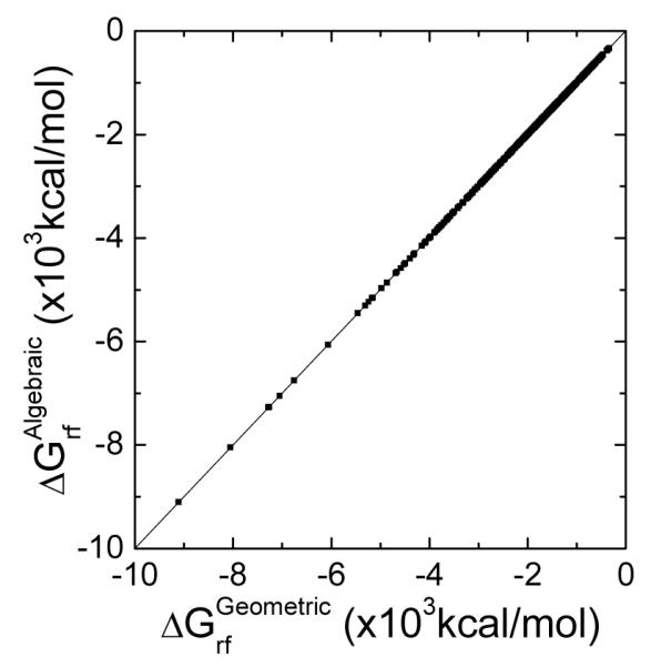
Correlation of reaction field energies by the geometric and algebraic methods for the 579 biomolecules in the Amber training set. Here the geometric and algebraic methods were used, respectively, to compute the intersection points of the molecular surface and finite-difference grid edges. The WHA method was used for the dielectric constant assignment on the molecular surface.

Our observed high-level consistency, in part, demonstrates the robustness in the implicit representation of surface with the level set method. Of course, the advantage of the algebraic method lies in its simplicity and the algebraic method is straightforward to be incorporated into the finite-difference methods. In contrast, the geometric method relies on the thoroughness of the rules or logics to enumerate all possibilities, leading to very complicated computer programs.

Convergence with respect to numerical resolution in solvent accessible arcs

Given the above consistency check and validation of different numerical algorithms, we now address the more important issue of convergence and stability of the numerical reaction field energies in the finite-difference methods. A high resolution in the numerical arc representation leads to a more accurate dielectric constant assignment, and thus more accurate reaction field energies, but it also requires more memory. The probe arcs used to build the solvent excluded surface increase quadratically with the atom number N_atom. As a consequence, finer resolution of discretized arcs leads to the computational complexity growth and run-time memory growth of $O\left(N_{atom}^2\right)$. However, we also need to bear in mind that the final accuracy of the reaction field energies also depends on the grid spacing. Thus it is necessary to identify which resolution, grid spacing or arc resolution, plays a more important role in the convergence accuracy of the numerical reaction field energies.

Figure 5 plots the relative convergence errors in the reaction field energies for the GC base pair with respect to the reference value computed at the grid spacing of 1/16 Å and a very high arc resolution of 1/256 Å. To explicitly show the benefit of the trimer arc points, we conducted the same calculation with the trimer arc dots and without the trimer arc dots. This analysis shows that both grid spacing and arc resolution influence the accuracy of the final computed reaction field energy. However, when the arc resolution reaches certain threshold, the grid spacing becomes the dominant factor, as indicated by the virtually horizontal contour lines in relative errors on the right part of the plot. For example, without the trimer arc dots, the threshold is 1/16 Å, while inclusion of the trimer arc dots lowers the threshold from 1/16 Å to 1/8 Å. In reality, we recommend setting the arc resolution to be max(h/2, 1/8 Å) with the trimer arc dots included and max(h/4, 1/16 Å) without the trimer arc dots.

Figure 5.

The relative errors in the reaction field energies of the GC base pair calculated by the algebraic method with different combinations of grid spacings and arc resolutions. (top: without the trimer arc dots; bottom: with the trimer arc dots) The unit of in-plot label is percent and the interval of the contour levels is 2%. Here the WHA method was used for the dielectric constant assignment on the molecular surface.

Table 1 supports our claim that inclusion of trimer dots can reduce run-time memory allocation by about half and the efficiency is little changed. The tests were performed with trimer arc dots and without trimer arc dots, respectively. Given the conclusion from the previous test and the grid spacing of 1/2 Å, we set the arc resolution to 1/4 Å if trimer arc dots are present and to 1/8 Å if there are no trimer arc dots to reach similar accuracy in the reaction field energy. Only the allocated memory during the arc dot calculation is shown here. The timing shown here has two portions, one from the arc dot generation and the other from gird point labeling, both of which are affected by the number of arc dots. Because the search for trimer arc dots of one atom need to consider all nearby three-atom groups with this atom as a member, the timing of calculating arc dots for this case is probably longer. However, it decreases the work load at the step of grid point labeling because fewer arc dots are looped over to determine the solute/solvent property of each grid point.

Table 1.

Comparison of memory and timing usage between finite difference SES definitions with and without trimer arc dots. The tested molecule is 1tsr, which has 3010 atoms. The timings were obtained from an average of three runs. The memory amounts were obtained from allocation requests in the code.

		With trimer arc dots	Without trimer arc dots
Memory (MB)		611	1123
Timing (s)	Arc dots calculations	0.76	0.63
	Grid point labeling	1.60	1.84
	Total	2.36	2.47

We also studied the quality of numerical force calculation with respect to the use of trimer arc dots. Figure 6 compares the accuracy in the total force on G of the GC dimer with and without the trimer arc dots. Note that the calculations were conducted at the typical coarse grid spacing of 1/2 Å. Apparently the numerical force is much more consistent with the virtual work force when trimer arc dots are present when the arc dot resolution is set to be 1/4 Å.

Figure 6.

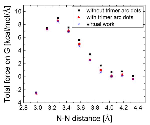
Total force on G of the GC dimer at different intra-molecular distances between G and C (the distance between N-1 of guanine and N-3 of cytosine). The grid spacing is 1/2 Å and the arc resolution is 1/4 Å. The forces computed with the virtual work principle are shown as a reference.

Table 2 further shows the uncertainties in numerical reaction field energies for both the GC base pair and the alanine-based helical hexamer. It is interesting to note that the uncertainties are mostly related to the grid spacing used. That is to say that given the same grid spacing, the standard deviations are mostly in the same order of magnitude no matter how fine the arc dot resolution is. Given that fine arc resolution does not help reduce the uncertainty in the numerical reaction field energy as shown in Table 2 and the analysis in Figure 5, our recommendation is to set the arc resolution to max(h/2, 1/8 Å) for typical grid spacings used in biomolecular applications. Of course this is with the trimer arc dots included. When the trimer arc dots are not included, the arc dot resolution should be reduced to max(h/4, 1/16 Å) to achieve similar accuracy level.

Table 2.

Standard deviations in computed reaction field energies (σ, kcal/mol) versus grid spacings (h, Å) and arc resolutions (arc, Å).

Molecule	1/h	1/arc	σ (×10−3)
GC	2	2	205.263
		4	206.637
		8	206.666
		16	206.773
	4	2	61.760
		4	61.774
		8	61.792
		16	61.713
	8	2	15.683
		4	15.722
		8	15.698
		16	15.708
A6α	2	2	103.671
		4	104.039
		8	103.782
		16	103.891
	4	2	29.457
		4	29.417
		8	29.367
		16	29.342
	8	2	6.488
		4	6.397
		8	6.432
		16	6.413

Convergence improvement with harmonic averaging of boundary dielectrics

It has been pointed out that the use of surface polarization charges can lead to much reduced grid dependence in numerical reaction field energies.²⁷ In this study, we further explored to combine harmonic averaging in boundary dielectrics with the “charge-based” approach to improve the convergence and to reduce the uncertainty of numerical reaction field energies and solvation forces.

It is often the case that reaction field energies converge in O(h²). Interestingly, only the convergence rate of the charge-based approach with WHA (both the geometric and algebraic implementations) is quadratic (Figure 7 top). The reaction field energy with the NHA scheme is linearly dependent on the grid spacing, and the reaction field energy with the SHA scheme follows a strange trend, i.e., at the coarsest grid spacing tested, the result is closer to the converged value than those at 1/4 Å and 1/8 Å. Accordingly, the SHA scheme performs the best at the 1/2 Å. Note that all of the three schemes converges to the consistent values as the grid spacing approaches zero.

Figure 7.

Effect of boundary dielectric constant assignments upon the convergence of reaction field energy (top), total reaction field force (middle), and total dielectric boundary force (bottom) for the GC base pair. Overall, the use of WHA offers the best convergence in the reaction field energies and solvation forces. Both algebraic and geometric methods were tested for the WHA approach. Their trends virtually overlap with each other. In all plots, standard deviations are plotted as error bars.

The standard deviations of the reaction field energies by different combinations of numerical methods are summarized in Table 3. Either the charge-view method or the WHA strategy alone can significantly reduce the grid dependence compared to the conventional field-view method and the NHA strategy. The total effect is a factor of three to five, depending on the grid spacing, and the most dramatic improvement happens at the coarsest grid spacing, i.e., 1/2 Å. Plus, the coarse-grid convergence of the combined strategy is better than that of any other numerical method, i.e., the numerical result at 1/2 Å is closest to the corresponding value at 1/16 Å.

Table 3.

Computed reaction field energies (ΔG_rf, kcal/mol) and its standard deviations (σ, kcal/mol) using the field-view and charge-view methods versus grid spacing (h, Å). The arc resolution is set as 1/16 Å.

Molecule	1/h	Δ Grfa	σ (×10−3)	Δ Grfb	σ (×10−3)	Δ Grfc	σ (×10−3)	Δ Grfd	σ (×10−3)
GC	2	−33.5242	206.773	−35.0113	332.501	−35.5759	426.927	−39.7517	1015.210
	4	−33.8544	61.713	−34.5456	80.032	−34.1831	120.799	−36.0042	189.163
	8	−33.9572	15.708	−34.2912	21.782	−34.0283	29.250	−34.9375	51.143
	16	−33.9852	3.537	−34.1493	5.815	−34.0030	6.534	−34.4608	13.057

ΔG_rf^a: Computed reaction field energies by charge-view method and WHA

ΔG_rf^b: Computed reaction field energies by charge-view method and NHA

ΔG_rf^c: Computed reaction field energies by field-view method and WHA

ΔG_rf^d: Computed reaction field energies by field-view method and NHA

It is also interesting that the solvation forces converge faster than the reaction field energies (Figure 7 middle), but the standard deviations of the solvation forces are always notably larger than those of the reaction field energies. For the reaction field forces, all of the three schemes converge super-quadratically and to the almost identical values (Table 4). Speaking of the dielectric boundary forces, both WHA and NHA can converge to reasonable values. Specifically, the relative difference between the two types of forces, the reaction field force and the dielectric boundary force, which are supposed to be virtually identical (the ionic boundary force is ~O(10^/2) smaller), is 1.3% for WHA and 4.8% for NHA. In contrast, SHA converges to a much lower value than the reaction field force, implying poor self-consistency with this scheme. In summary, the WHA method leads to the smallest uncertainties in both energies and forces of the tested molecule.

Table 4.

Parameters in fitting curves of reaction field energies (ΔG_rf), total reaction field forces (F_rf) and total dielectric boundary forces (F_db) of the GC dimer. The function of fitting curves is y = a + bx^c.

	Dielectrica assignment	a	δa	b	δb	c	δc
ΔGrf	WHA	−33.99704	0.00099	1.64453	0.09171	1.78244	0.04528
	SHA	−28.83106	287.21239	−5.47042	287.03984	0.01507	0.81940
	NHA	−33.97263	0.00232	−1.86529	0.01356	0.85012	0.00712
Frf	WHA	2.91524	0.00057	1.39715	0.55563	2.99490	0.42248
	SHA	2.91666	0.00033	1.45674	0.08986	2.30441	0.05383
	NHA	2.92084	0.00028	7.00734	0.57384	3.49764	0.09470
Fdb	WHA	2.87835	0.00104	2.33396	0.23610	1.98509	0.06891
	SHA	2.38492	0.00307	4.48417	2.83767	3.85429	0.87303
	NHA	3.06012	0.00892	4.28107	0.73432	1.80266	0.14246

Finally Figure 8 illustrates the consistency of electrostatic solvation forces calculated by different boundary dielectric constant assignments at the finest grid spacing tested (1/16 Å). Overall, there is a high-level consistency between the algebraic method and the geometric method in both reaction field forces and dielectric boundary forces. Furthermore, the WHA approach leads to the lowest numerical uncertainties in computed forces, especially the dielectric boundary forces (about ten times smaller).

Figure 8.

Consistency of electrostatic solvation forces calculated by different boundary dielectric constant assignments at the finest tested grid spacing of 1/16 Å. Top: atomic reaction field forces and their standard deviations. Bottom: atomic dielectric boundary forces and their standard deviations.

Timing analysis

In the charge-view method, extra time is needed on the computation of polarizable charges on the interface. It is important to know the timing expense of the charge-view method, compared to the total FDPB timing. Figure 9 shows that the ratio of the charge-view timing and the total timing grows substantially with the grid size at the beginning, and later becomes stable at around 23% with small fluctuations. Thus the benefit still outweighs the cost for most tested molecules given that the same accuracy level can only be achieved with a smaller grid spacing. For example, a grid spacing of 1/3 Å is necessary for the classical method to achieve comparable results with the charge-view method at the grid spacing of 1/2 Å. The finer grid clearly leads to a linear system about four times larger, and roughly four times more CPU time is needed to solve the linear system because the bottleneck of the new method is still the linear system solver (at least 75% for the largest linear system).

Figure 9.

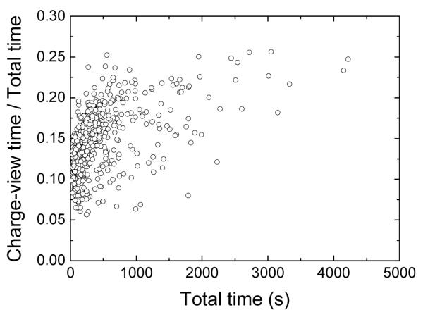
The ratio of the charge-view time and the total PBSA time versus the total PBSA time.

Possible extension to full PB systems

It is expected that the charge-view method will become more complicated when applied to the full PB equation. There would be much more pair-wise additions after the mobile charges are included. Although we can use fast Fourier transform to speed up the calculations, there is actually no need to do so.

The total electrostatic energy in the presence of mobile charges can be computed with the following field-view formula:⁷⁷

$$G=\int \left(\frac{{\rho }^f\varphi }{2}-\frac{{\rho }^m\varphi }{2}-\Delta \Pi \lambda \right)dv$$ (9)

The first term is the energy associated with the fixed charges, the second term is the energy associated with the mobile charges, and the last term is the entropic term due to the osmotic excess pressure. Here ρ_f is the fixed charge density, ρ_m is the mobile charge density, φ the total potential, which can be decomposed into three parts as follows

$$\varphi ={\varphi }_C^f+{\varphi }_C^m+{\varphi }_{RF}$$ (10)

where ${\varphi }_C^f$ is the potential due to the fixed charges, ${\varphi }_C^m$ is the potential due to the mobile charges, φ_RF is the reaction field potential in the full PB system. The third term in eqn (9) is the entropic term due to the excess osmotic pressure, apparently not due to charge-charge interactions so that no further treatment will be attempted.. The second term in eqn (9) can be computed as present in the current form because the potential is weak due to solvent screening. Thus our focus is on how to compute the first term in eqn (9) more accurately in the current effort.

According to eqn (10), the first term can be further split into three parts, the interactions between atomic charges, the interactions between atomic charges and mobile charges, and the interactions between atomic charges and polarization charges, i.e.,

$$G^f=\frac{1}{2}\int {\rho }^f\varphi dv=\frac{1}{2}\int {\rho }^f({\varphi }_C^f+{\varphi }_C^m+{\varphi }_{RF})dv$$ (11)

The motivation in replacing the field-view method with the charge-view method is to reduce the finite difference error, especially the error in the potential nearby the atomic charges. Thus the best improvement in applying the charge-view method is to charges that are close to each other, typically within a cutoff distance of R_cut. For charges that are far away from each other, apparently the field-view method still works well. This particle-particle particle-mesh (P3M) strategy would greatly simplify the full charge-view method without much sacrifice in accuracy.⁷⁸ Thus eqn (11) is modified to

$$G^f=\frac{1}{2}\int {\rho }^f\varphi dv-(G_C^{short}+G_{pol}^{short})+G_{pair}^{short}$$ (12)

where $G_C^{short}=\frac{1}{2}\int {\rho }^f{\varphi }_C^{short}dv$ is the short-range interactions between atomic charges, $G_{pol}^{short}=\frac{1}{2}\int {\rho }^f{\varphi }_{RF}dv$ is the short-range interactions between atomic charges and polarizable charges. These two field-view terms are computed by Luty et al’s approach⁷⁹ and then subtracted from G_f because they are the least accurate and substituted by the pair-wise charge-charge interactions, i.e.,

$$G_{pair}^{short}=\frac{1}{2{\epsilon }_{in}}\sum _i\sum _j\frac{q_i{q}_j}{r_{ij}}+\frac{1}{2}\sum _i\sum _j\frac{q_i{q}_j^{pol}}{r_{ij}^{\prime }}$$ (13)

where q_i, q_j are the atomic charges, r_ij are the distances between atomic charges i and j, $r_{ij}^{\prime }$ are the distances between atomic charges and polarizable charges. The integral interval in eqn (12) and summation terms in eqn (13) are determined by the short-range cutoff distance R_cut.

The above P3M strategy was compared with the field-view method on the computation of the total electrostatic energies of small molecules. The convergence behaviors of the two methods are shown in Figure 10. The charge-view result is also plotted as a reference. Because the energies were computed from the solutions of a linearized PB equation, only the first term in eqn (9) remains. As expected, the P3M strategy has less convergence error at coarse grid spacings and half-reduced uncertainties in the reaction field energies for both tested small molecules. The high consistency between the charge-view method and the P3M indicates that the particle mesh method to compute the interactions between charges at a distance remains to be a good approximation.

Figure 10.

Reaction field energies of two small molecules in a water environment with continuum ions. Linearized PB equations were solved before the reaction field energy calculation. The ion strength is 0.15 M. Three different methods were applied and shown in the figure for comparison (all with the WHA scheme). Top: GC dimer; Bottom: A6_α.

Limitations and future directions

As reviewed in the Introduction the solvent excluded surface has been widely adopted for numerical PB methods in biomolecular applications involving static structures. However it still requires more development to adopt the SES definition for molecular dynamics simulations.⁶¹ Indeed, difficulty was also observed in the pair-wise generalized Born (GB) method when the SES definition was used for biomolecular dynamics simulations.⁸⁰ A major limitation of the SES definition is the reentry volume: it is found that large reentry volume generated by non-bonded atoms comes and goes as often as every femtosecond when the nearby atoms undergo vibrational motion in simulations of proteins at room temperature.⁶¹ Thus extremely large surface derivatives with respect to atomic coordinates may occur in the SES definition. In addition, surface cusp may also exist given certain combinations of atom and probe radii and arrangements of atoms. Finally, partition of dielectric boundary force elements on the solvent/surface interface to nearby atoms is also crucially important when the numerical PB methods can be applied to routine energy minimization and molecular dynamics simulations. These limitations require us to redefine the molecular surface that is both smooth and differentiable with respect to the atomic positions. Thus how to preserve the good physical properties of the SES definition in the development of a smooth and differentiable surface definition is clearly an important future direction. It should be pointed out that several recent developments were also reported to smooth the SES surface,^81-85 which should also be investigated in the future.

Conclusions

In this study we have discussed our strategies to overcome the numerical difficulties associated with the solvent excluded surface definition in the finite-difference Poisson-Boltzmann methods. Specifically we have developed new numerical procedures and explored strategies to minimize the dependence in the numerical energies and forces upon grid resolution.

To map the grid-independent solvent excluded surface to the finite-difference grid, we have proposed an algebraic method that utilizes the concept of the level set function to trace the molecular surface implicitly. The advantage of the algebraic approach lies in its simple logics leading to efficient implementation. Of course a high level of consistency does exist between the algebraic method and the classical method as has been demonstrated with a diversified test set of biomolecules.

Next we have addressed the more important issue of convergence and stability of the numerical reaction field energies and solvation forces when the solvent excluded surface is used in the finite-difference methods. We found that both grid spacing and solvent accessible arc resolution influence the accuracy of the final computed reaction field energy for a tested molecular system, and inclusion of trimer arc dots during surface generation is beneficial to the convergence of both reaction field energies and solvation forces given the same arc resolution. In addition, the uncertainties in the numerical reaction field energies for tested molecules are mostly related to the grid spacing used even when the arc resolution is comparable to the grid spacing.

We have further explored to combine harmonic averaging in boundary dielectrics with the “charge-based” approach to improve the convergence of numerical reaction field energies and solvation forces and to reduce their uncertainties. Interestingly, the use of surface polarization charges changes the convergence behaviors of the reaction field energies and solvation forces. In addition, the weighted harmonic averaging method leads to the smallest numerical uncertainty in both energy and force calculation. The combined strategy can also be extended to the full PB equation. The P3M method has been proved to be able to improve the efficiency with negligible loss of accuracy.

References

- (1).Davis ME, McCammon JA. Chem. Rev. 1990;90:509. [Google Scholar]
- (2).Sharp KA. Curr. Opin. Struct. Biol. 1994;4:234. [Google Scholar]
- (3).Gilson MK. Curr. Opin. Struct. Biol. 1995;5:216. doi: 10.1016/0959-440x(95)80079-4. [DOI] [PubMed] [Google Scholar]
- (4).Honig B, Nicholls A. Sci. 1995;268:1144. doi: 10.1126/science.7761829. [DOI] [PubMed] [Google Scholar]
- (5).Roux B, Simonson T. Biophys. Chem. 1999;78:1. doi: 10.1016/s0301-4622(98)00226-9. [DOI] [PubMed] [Google Scholar]
- (6).Cramer CJ, Truhlar DG. Chem. Rev. 1999;99:2161. doi: 10.1021/cr960149m. [DOI] [PubMed] [Google Scholar]
- (7).Bashford D, Case DA. Annu. Rev. Phys. Chem. 2000;51:129. doi: 10.1146/annurev.physchem.51.1.129. [DOI] [PubMed] [Google Scholar]
- (8).Baker NA. Curr. Opin. Struct. Biol. 2005;15:137. doi: 10.1016/j.sbi.2005.02.001. [DOI] [PubMed] [Google Scholar]
- (9).Chen JH, Im WP, Brooks CL. J. Am. Chem. Soc. 2006;128:3728. doi: 10.1021/ja057216r. [DOI] [PMC free article] [PubMed] [Google Scholar]
- (10).Feig M, Chocholousova J, Tanizaki S. Theor. Chem. Acc. 2006;116:194. [Google Scholar]
- (11).Im W, Chen JH, Brooks CL. Peptide Solvation and H/Bonds. 2006;72:173. [Google Scholar]
- (12).Koehl P. Curr. Opin. Struct. Biol. 2006;16:142. doi: 10.1016/j.sbi.2006.03.001. [DOI] [PubMed] [Google Scholar]
- (13).Lu BZ, Zhou YC, Holst MJ, McCammon JA. Commun. Comput. Phys. 2008;3:973. [Google Scholar]
- (14).Wang J, Tan CH, Tan YH, Lu Q, Luo R. Commun. Comput. Phys. 2008;3:1010. [Google Scholar]
- (15).Warwicker J, Watson HC. J. Mol. Biol. 1982;157:671. doi: 10.1016/0022-2836(82)90505-8. [DOI] [PubMed] [Google Scholar]
- (16).Davis ME, McCammon JA. J. Comput. Chem. 1989;10:386. [Google Scholar]
- (17).Klapper I, Hagstrom R, Fine R, Sharp K, Honig B. Proteins Structure Function and Genetics. 1986;1:47. doi: 10.1002/prot.340010109. [DOI] [PubMed] [Google Scholar]
- (18).Luty BA, Davis ME, McCammon JA. J. Comput. Chem. 1992;13:1114. [Google Scholar]
- (19).Nicholls A, Honig BJ. Comput. Chem. 1991;12:435. [Google Scholar]
- (20).Forsten KE, Kozack RE, Lauffenburger DA, Subramaniam S. J. Phys. Chem. 1994;98:5580. [Google Scholar]
- (21).Holst M, Saied F. J. Comput. Chem. 1993;14:105. [Google Scholar]
- (22).Im W, Beglov D, Roux B. Comput. Phys. Commun. 1998;111:59. [Google Scholar]
- (23).Rocchia W, Alexov E, Honig B. J. Phys. Chem. B. 2001;105:6507. [Google Scholar]
- (24).Bashford D. Lecture Notes in Computer Science. 1997;1343:233. [Google Scholar]
- (25).Gilson MK, Sharp KA, Honig BH. J. Comput. Chem. 1988;9:327. [Google Scholar]
- (26).Luo R, David L, Gilson MK. J. Comput. Chem. 2002;23:1244. doi: 10.1002/jcc.10120. [DOI] [PubMed] [Google Scholar]
- (27).Rocchia W, Sridharan S, Nicholls A, Alexov E, Chiabrera A, Honig B. J. Comput. Chem. 2002;23:128. doi: 10.1002/jcc.1161. [DOI] [PubMed] [Google Scholar]
- (28).Madura JD, Briggs JM, Wade RC, Davis ME, Luty BA, Ilin A, Antosiewicz J, Gilson MK, Bagheri B, Scott LR, McCammon JA. Computer Physics Communications. 1995;91:57. [Google Scholar]
- (29).Nicholls A, Sharp KA, Honig B. Proteins/Structure Function and Genetics. 1991;11:281. doi: 10.1002/prot.340110407. [DOI] [PubMed] [Google Scholar]
- (30).Wang J, Cai Q, Li ZL, Zhao HK, Luo R. Chem. Phys. Lett. 2009;468:112. doi: 10.1016/j.cplett.2008.12.049. [DOI] [PMC free article] [PubMed] [Google Scholar]
- (31).Cai Q, Wang J, Zhao HK, Luo R. Journal of Chemical Physics. 2009;130:145101. doi: 10.1063/1.3099708. [DOI] [PubMed] [Google Scholar]
- (32).Baker N, Holst M, Wang F. J. Comput. Chem. 2000;21:1343. [Google Scholar]
- (33).Cortis CM, Friesner RA. J. Comput. Chem. 1997;18:1591. [Google Scholar]
- (34).Holst M, Baker N, Wang F. J. Comput. Chem. 2000;21:1319. [Google Scholar]
- (35).Chen L, Holst MJ, Xu JC. SIAM J. Numer. Anal. 2007;45:2298. [Google Scholar]
- (36).Shestakov AI, Milovich JL, Noy A. J. Colloid Interface Sci. 2002;247:62. doi: 10.1006/jcis.2001.8033. [DOI] [PubMed] [Google Scholar]
- (37).Xie D, Zhou S. BIT Numerical Mathematics. 2007;47:853. [Google Scholar]
- (38).Hoshi H, Sakurai M, Inoue Y, Chujo R. J. Chem. Phys. 1987;87:1107. [Google Scholar]
- (39).Miertus S, Scrocco E, Tomasi J. Chem. Phys. 1981;55:117. [Google Scholar]
- (40).Zauhar RJ, Morgan RS. J. Comput. Chem. 1988;9:171. [Google Scholar]
- (41).Juffer AH, Botta EFF, Vankeulen BAM, Vanderploeg A, Berendsen HJC. J. Comput. Phys. 1991;97:144. [Google Scholar]
- (42).Rashin AA. J. Phys. Chem. 1990;94:1725. [Google Scholar]
- (43).Yoon BJ, Lenhoff AM. J. Comput. Chem. 1990;11:1080. [Google Scholar]
- (44).Bharadwaj R, Windemuth A, Sridharan S, Honig B, Nicholls A. J. Comput. Chem. 1995;16:898. [Google Scholar]
- (45).Purisima EO, Nilar SH. J. Comput. Chem. 1995;16:681. [Google Scholar]
- (46).Zhou HX. Biophys. J. 1993;65:955. doi: 10.1016/S0006-3495(93)81094-4. [DOI] [PMC free article] [PubMed] [Google Scholar]
- (47).Liang J, Subramaniam S. Biophys. J. 1997;73:1830. doi: 10.1016/S0006-3495(97)78213-4. [DOI] [PMC free article] [PubMed] [Google Scholar]
- (48).Vorobjev YN, Scheraga HA. J. Comput. Chem. 1997;18:569. [Google Scholar]
- (49).Boschitsch AH, Fenley MO, Zhou HX. J. Phys. Chem. B. 2002;106:2741. [Google Scholar]
- (50).Lu BZ, Cheng XL, Huang JF, McCammon JA. Proc. Natl. Acad. Sci. U. S. A. 2006;103:19314. doi: 10.1073/pnas.0605166103. [DOI] [PMC free article] [PubMed] [Google Scholar]
- (51).Totrov M, Abagyan R. Biopolymers. 2001;60:124. doi: 10.1002/1097-0282(2001)60:2<124::AID-BIP1008>3.0.CO;2-S. [DOI] [PubMed] [Google Scholar]
- (52).Richards FM. Annual Review of Biophysics and Bioengineering. 1977;6:151. doi: 10.1146/annurev.bb.06.060177.001055. [DOI] [PubMed] [Google Scholar]
- (53).Connolly ML. J. Appl. Crystallogr. 1983;16:548. [Google Scholar]
- (54).Connolly ML. Science. 1983;221:709. doi: 10.1126/science.6879170. [DOI] [PubMed] [Google Scholar]
- (55).Swanson JMJ, Mongan J, McCammon JA. J. Phys. Chem. B. 2005;109:14769. doi: 10.1021/jp052883s. [DOI] [PubMed] [Google Scholar]
- (56).Tan CH, Yang LJ, Luo R. J. Phys. Chem. B. 2006;110:18680. doi: 10.1021/jp063479b. [DOI] [PubMed] [Google Scholar]
- (57).Wang J, Tan C, Chanco E, Luo R. Physical Chemistry Chemical Physics. 2010;12 doi: 10.1039/b917775b. In press. [DOI] [PubMed] [Google Scholar]
- (58).Zauhar RJ, Morgan RS. J. Comput. Chem. 1990;11:603. [Google Scholar]
- (59).Eisenhaber F, Argos P. J. Comput. Chem. 1993;14:1272. [Google Scholar]
- (60).You T, Bashford DJ. Comput. Chem. 1995;16:743. [Google Scholar]
- (61).Lu Q, Luo R. J. Chem. Phys. 2003;119:11035. [Google Scholar]
- (62).Grant JA, Pickup BT, Nicholls A. J. Comput. Chem. 2001;22:608. [Google Scholar]
- (63).Grant JA, Pickup BT. Journal of Physical Chemistry. 1995;99:3503. [Google Scholar]
- (64).Ye X, Wang J, Luo R. Journal of Chemical Theory and Computation. 2010;6:1157. doi: 10.1021/ct900318u. [DOI] [PMC free article] [PubMed] [Google Scholar]
- (65).Davis ME, McCammon JA. J. Comput. Chem. 1991;12:909. [Google Scholar]
- (66).Mohan V, Davis ME, McCammon JA, Pettitt BM. J. Phys. Chem. 1992;96:6428. [Google Scholar]
- (67).Kottmann ST. Theor. Chem. Acc. 2008;119:421. [Google Scholar]
- (68).Bruccoleri RE, Novotny J, Davis ME. J. Comput. Chem. 1997;18:268. [Google Scholar]
- (69).Cai Q, Ye X, Wang J, Luo R. Chem. Phys. Let. 514:368. doi: 10.1016/j.cplett.2011.08.067. [DOI] [PMC free article] [PubMed] [Google Scholar]
- (70).Osher S, Fedkiw RP. Level set methods and dynamic implicit surfaces. Springer; New York: 2003. [Google Scholar]
- (71).Sethian JA. Level set methods and fast marching methods : evolving interfaces in computational geometry, fluid mechanics, computer vision, and materials science. Cambridge University Press; Cambridge, U.K.; New York: 1999. [Google Scholar]
- (72).Can T, Chen CI, Wang YF. J. Mol. Graph. 2006;25:442. doi: 10.1016/j.jmgm.2006.02.012. [DOI] [PubMed] [Google Scholar]
- (73).Landau LD, Lifshitz EM, Pitaevskii LP. [Google Scholar]
- (74).Gilson MK, Davis ME, Luty BA, McCammon JA. J. Phys. Chem. 1993;97:3591. [Google Scholar]
- (75).Case DA, Cheatham TE, Darden T, Gohlke H, Luo R, Merz KM, Onufriev A, Simmerling C, Wang B, Woods RJ. Journal of Computational Chemistry. 2005;26:1668. doi: 10.1002/jcc.20290. [DOI] [PMC free article] [PubMed] [Google Scholar]
- (76).Case DA, Darden TA, Cheatham TE, III, Simmerling CL, Wang J, Duke RE, Luo R, Crowley M, Walker RC, Zhang W, Merz KM, Wang B, Hayik A, Roitberg A, Seabra G, Kolossvary I, Wong KF, Paesani F, Vanicek J, X W, Brozell SR, Steinbrecher T, Gohlke H, Yang L, Tan C, Mongan J, Hornak V, Cui G, Mathews DH, Seetin MG, Sagui C, Babin V, Kollman PA. 10 ed The Regents of the University of California; San Francisco: 2008. [Google Scholar]
- (77).Sharp KA, Honig B. J. Phys. Chem. 1990;94:7684. [Google Scholar]
- (78).Ye X, Cai Q, Luo R. in preparation. [Google Scholar]
- (79).Luty BA, Davis ME, McCammon JA. Journal Of Computational Chemistry. 1992;13:768. [Google Scholar]
- (80).Chocholousova J, Feig M. J. Comput. Chem. 2006;27:719. doi: 10.1002/jcc.20387. [DOI] [PubMed] [Google Scholar]
- (81).Vorobjev YN, Hermans J. Biophys. J. 1997;73:722. doi: 10.1016/S0006-3495(97)78105-0. [DOI] [PMC free article] [PubMed] [Google Scholar]
- (82).Cheng HL, Dey TK, Edelsbrunner H, Sullivan J. Discrete & Computational Geometry. 2001;25:525. [Google Scholar]
- (83).Cheng HL, Shi XW. Computational Geometry/Theory and Applications. 2009;42:196. [Google Scholar]
- (84).Edelsbrunner H. Discrete & Computational Geometry. 1999;21:87. doi: 10.1007/s00454-021-00281-9. [DOI] [PMC free article] [PubMed] [Google Scholar]
- (85).Shi XW, Koehl P. Communications in Computational Physics. 2008;3:1032. [Google Scholar]
Associated Data
This section collects any data citations, data availability statements, or supplementary materials included in this article.