Transition paths, diffusive processes, and preequilibria of protein folding

Abstract

Fundamental relationships between the thermodynamics and kinetics of protein folding were investigated using chain models of natural proteins with diverse folding rates by extensive comparisons between the distribution of conformations in thermodynamic equilibrium and the distribution of conformations sampled along folding trajectories. Consistent with theory and single-molecule experiment, duration of the folding transition paths exhibits only a weak correlation with overall folding time. Conformational distributions of folding trajectories near the overall thermodynamic folding/unfolding barrier show significant deviations from preequilibrium. These deviations, the distribution of transition path times, and the variation of mean transition path time for different proteins can all be rationalized by a diffusive process that we modeled using simple Monte Carlo algorithms with an effective coordinate-independent diffusion coefficient. Conformations in the initial stages of transition paths tend to form more nonlocal contacts than typical conformations with the same number of native contacts. This statistical bias, which is indicative of preferred folding pathways, should be amenable to future single-molecule measurements. We found that the preexponential factor defined in the transition state theory of folding varies from protein to protein and that this variation can be rationalized by our Monte Carlo diffusion model. Thus, protein folding physics is different in certain fundamental respects from the physics envisioned by a simple transition-state picture. Nonetheless, transition state theory can be a useful approximate predictor of cooperative folding speed, because the height of the overall folding barrier is apparently a proxy for related rate-determining physical properties.

Protein folding is an intriguing phenomenon at the interface of physics and biology. In the early days of folding kinetics studies, folding was formulated almost exclusively in terms of mass-action rate equations connecting the folded, unfolded, and possibly, one or a few intermediate states (1, 2). With the advent of site-directed mutagenesis, the concept of free energy barriers from transition state theory (TST) (3) was introduced to interpret mutational data (4), and subsequently, it was adopted for the Φ-value analysis (5). Since the 1990s, the availability of more detailed experimental data (6), in conjunction with computational development of coarse-grained chain models, has led to an energy landscape picture of folding (7–15). This perspective emphasizes the diversity of microscopic folding trajectories, and it conceptualizes folding as a diffusive process (16–25) akin to the theory of Kramers (26).

For two-state-like folding, the transition path (TP), i.e., the sequence of kinetic events that leads directly from the unfolded state to the folded state (27, 28), constitutes only a tiny fraction of a folding trajectory that spends most of the time diffusing, seemingly unproductively, in the vicinity of the free energy minimum of the unfolded state. The development of ultrafast laser spectroscopy (29, 30) and single-molecule (27, 28, 31) techniques have made it possible to establish upper bounds on the transition path time (t_TP) ranging from <200 and <10 μs by earlier (27) and more recent (28), respectively, direct single-molecule FRET to <2 μs (30) by bulk relaxation measurements. Consistent with these observations, recent extensive atomic simulations have also provided estimated t_TP values of the order of ∼1 μs (32, 33). These advances offer exciting prospects of characterizing the productive events along folding TPs.

It is timely, therefore, to further the theoretical investigation of TP-related questions (19). To this end, we used coarse-grained C_α models (14) to perform extensive simulations of the folding trajectories of small proteins with 56- to 86-aa residues. These tractable models are useful, because despite significant progress, current atomic models cannot provide the same degree of sampling coverage for proteins of comparable sizes (32, 33). In addition to structural insights, this study provides previously unexplored vantage points to compare the diffusion and TST pictures of folding. Deviations of folding behaviors from TST predictions are not unexpected, because TST is mostly applicable to simple gas reactions; however, the nature and extent of the deviations have not been much explored. Our explicit-chain simulation data conform well to the diffusion picture but not as well to TST. In particular, the preexponential factors of the simulated folding rates exhibit a small but appreciable variation that depends on native topology. These findings and others reported below underscore the importance of single-molecule measurements (13, 27, 28, 31, 34, 35) in assessing the merits of proposed scenarios and organizing principles of folding (7–25, 36, 37).

Results

Our approach is outlined in Methods; additional details are provided in SI Text. Coarse-grained models (14, 38) were used for explicit-chain simulations. Like before (39, 40), the fractional number of native contacts, Q, was used as a progress variable (41). Extensive statistics on folding path (FP), first passage time (FPT), TP, and (Fig. 1) were collected for eight model proteins (Table S1). To assess the diffusion picture of folding (16–25), we compared the explicit-chain simulation results with the results from a simple 1D nonexplicit-chain Monte Carlo (MC) process with an effective constant diffusion coefficient D₀. The MC simulations do not address structural questions but are important for conceptual understanding of the distributions of FPT and values. In general, diffusion coefficients for folding are Q-dependent (20, 22), and formulations are available for computing D(Q) from chain simulation data (22, 42). Here, we find it enlightening to use an even simpler diffusion picture, which is exemplified by other simple diffusion models of folding (21, 43, 44). Additional exposition of our rationale is provided in SI Text.

Fig. 1.

FPT and t_TP illustrated using model 2CI2 simulated at the transition midpoint. (A) The TP (red trace) is the last part of an example folding trajectory (FP, black trace plus red trace) with an FPT ≈ 2.7 × 10⁷. The rest of the equilibrium fluctuation is shown in gray. (B) The TP in A plotted in an expanded horizontal scale shows that the model protein makes a transition from Q_D = 0.122 to Q_N = 1 during a t_TP ≈ 4.6 × 10⁴.

Statistics of Folding Trajectories Are Better Described by Conformational Diffusion than the TST Picture.

TST envisions a preequilibrium in which the reactant states follow a Boltzmann distribution (3). In protein folding, it is often assumed that a preequilibrium is achieved by the folding trajectories in stopped-flow experiments (5). We test this idea (Fig. S1A) by comparing the thermodynamic free energy profile with kinetic (nonequilibrium) profiles (Fig. 2A) constructed from N folding trajectories labeled by i. Let be the FPT and be the time that the protein resides at Q in trajectory i. We computed two distributions, and . is proportional to the total residence time at Q for an ensemble of trajectories, resulting in more weights for longer trajectories, whereas gives equal weight to every trajectory. In principle, can be determined experimentally by ensemble measurements, whereas requires single-molecule measurements.

Fig. 2.

FPT and t_TP distributions. (A) Thermodynamic and kinetic FP profiles for model 2CI2. The simulated equilibrium free energy profile −lnP_eq(Q) + c (where c is a vertical shift; in the text) and the kinetic −lnP_FP(Q) and −lnP_FP|_s(Q) profiles are shown, respectively, by the black curve and the thin blue and red curves (c = −0.30). The corresponding nonexplicit-chain −lnP_FP(Q) and −lnP_FP|_s(Q) profiles obtained by MC simulations with an effective constant D₀ are shown by the thick blue and red curves (results from the Metropolis and Kawasaki algorithms are nearly identical). As expected, the thick blue curve coincides with the analytically derived −lnP_FP(Q) profile for constant diffusive coefficient D₀ (green curve). (B) Scatter plots of the explicit-chain simulated ‹t_TP› (in units of Langevin time steps) with (i) the nonexplicit-chain MC simulated ‹t_TP›_D0 by assuming a constant D₀ (red data points; top horizontal scale) (Fig. S2C; in units defined in the caption for Table S2) and (ii) a quantity in the Szabo formula quoted in ref. 27 (black data points; bottom horizontal scale) for the eight proteins studied, where ΔG^‡ is the thermodynamic free energy barrier in the explicit-chain model (Table S2). The red and black lines are the least-squares fits, with r = 0.94 and r = 0.78, respectively, for the data points plotted in the same color. (C) TPT distributions. For every protein, the range of simulated t_TP values was divided into 20 bins of equal size, Δt_TP. The simulated probability density is then provided by the normalized population of each bin divided by Δt_TP (shown here as data points). The continuous curves are two-parameter fits of the simulated t_TP/10⁵ values to equation 31 in the work by Malinin and Chernyak (47), and the fitted parameters are given in Fig. S2. (D) Scatter plot of explicit chain-simulated t_TP vs. FPT for model 2CI2 (r = −0.034).

If preequilibrium holds, the equilibrium and kinetic distributions should be identical for the unfolded conformations. Thus, their profiles should coincide in the unfolded region after vertical shifts are made to account for the differences in normalization [i.e., should overlap with for ] (Fig. S1A). For our model 2CI2 (Fig. 2A), the two profiles overlap for an extended region in the unfolded basin, but there are significant deviations near the equilibrium free energy barrier at . (A similar comparison for unfolding is given in Fig. S1B.) In Fig. 2A, the single-molecule profile (thin red curve) is lower than the ensemble kinetic profile (thin blue curve) for , indicating that longer trajectories spend proportionally less time in these Q values. The same trend is observed for other model proteins (Fig. S1C). The preequilibrium idea assumes that the variation of residence time relative to the mean residence time in every is equal to the variation of FPT relative to the mean FPT (MFPT). In contrast, our explicit-chain model results in Fig. 2A show that, proportionally, the variation of residence time in the barrier region is narrower than the variation of the FPT.

However, these behaviors are well-accounted for by a diffusive process: our nonexplicit-chain MC simulations (thick red and blue curves in Fig. 2A) reproduce the essentials of the explicit-chain kinetic profiles; the MC and explicit-chain MFPTs also correlate well (Fig. S2 A and B and Table S2). To pursue the diffusion picture further, we compare the MC-simulated with the analytical prediction from the Smoluchowski equation (Eq. 1):

where p(Q, t) is the probability density of Q at time t; , where k_B is the Boltzmann constant and T is absolute temperature; D(Q) and G(Q) are the Q-dependent diffusion coefficient and free energy, respectively; ; and . The quantity corresponding to is (Eq. 2)

for an initial distribution of 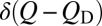at t = 0, with Q_N being a perfect absorber (16). θ is the Heaviside function. Applying Eq. 2 to discrete Q values (in incremental units of δQ) (Methods) for and assuming a Q-independent D₀ yields (Eq. 3)

Fig. 2A shows that this analytical profile (green curve) essentially coincides with the profile obtained from our MC simulation (thick blue curve), indicating that the latter is a good representation of a diffusive process governed by the Smoluchowski equation. As has been shown (16, 45, 46), Eq. 1 leads to the following general expression for MFPT of folding (Eq. 4):

which reduces to (Eq. 5)

when Q is discrete and is a constant. Thus, an effective constant diffusion coefficient can be defined using Eq. 5 when MFPT and are known (Fig. S2A).

The duration of a TP is only a tiny fraction of the folding time (Fig. 1); however, TPs are important, because they inform us how productive protein folding occurs. Fig. 2B shows that the variation in the average among the model proteins can be reasonably captured by a diffusion picture: our MC model (red data points) as well as the relation ‹t_TP› ≈ (2πF)⁻¹[ln(βΔG^‡) + constant] proposed by Szabo (27, 28), where is the free energy barrier. From the fitted curve to the black data points in Fig. 2B, the front factor F ≈ 4.6 × 10⁻⁶ estimated by this relation is smaller, but it is within less than one order of magnitude from the F^db ≈ 1.7 × 10⁻⁵ value estimated previously for a similar class of explicit-chain protein models (39). A possible origin of this minor mismatch will be discussed below. The distributions of our explicit-chain t_TP are also rationalizable by a diffusion picture: they are well-described by our MC simulations (Fig. S2D) and can be fitted (Fig. 2C) to an analytical formula for P(t_TP) derived (47) from a Fokker–Planck formulation (details in Fig. S2). The t_TP distribution recently obtained from a Gō model also exhibited a similar trend (24). Consistent with experiments (27, 28), t_TP is two or three orders smaller than FPT here. There is no correlation between t_TP and FPT (Fig. 2D and Fig. S3), indicating that the duration of productive folding is independent of the time spent in the largely unproductive conformational search.

Initial Stages of Transition Paths Have Statistically Atypical Contact Patterns.

Why do TPs succeed, whereas other much more common trajectories fail to reach the native structure? Do the conformations traversed by TPs constitute an ensemble of specific pathways that is fundamentally different from non-TP trajectories? We used two parameters to quantify the difference in conformational character between TPs and FPs: (i) ‹CO_TP›/‹CO_FP› is the average native contact order (CO) sampled along TPs divided by the average native contact order sampled along FPs, and (ii) is the mean square deviation of native contact probabilities sampled along TPs from the native contact probabilities achieved by FPs in the putative transition state at Q^‡ (Methods).

These two parameters show deviations of the conformational properties of TPs from the conformational properties of FPs in the folding quasi-preequilibrium (a quasi prefix is added because preequilibrium is not exact; see above). The observed deviations are insensitive to whether the averaging over FPs is normalized by individual FPT [as for P_FP|_s(Q)] or not [as for P_FP(Q)]. Remarkably, the deviations start at the earliest stage of the TPs. Fig. 3, Upper indicates that TPs tend to begin in the unfolded region with a higher contact order than a typical conformation in the quasi-preequilibrium with the same Q (‹CO_TP›/‹CO_FP› ≈ 1.07–1.1 at Q ≈ Q_D). As Q increases, the variation of ‹CO_TP›/‹CO_FP› can be mostly oscillatory (Fig. 3 A–C and E–G) or essentially monotonic (Fig. 3 D and H). Except for 1SHF (Fig. 3F), the ‹CO_TP›/‹CO_FP› ratio is larger than unity (with maximum values > 1.1 for most cases) for an extended range of Q < Q^‡. In three cases (1IMQ, 3GB1, and 1CSP), ‹CO_TP›/‹CO_FP› exhibits a high value of 1.12, 1.14, and 1.44 at Q ≈ 0.65, 0.62, and 0.51, respectively, just before Q^‡ is reached. Except for 1SHF, all other ‹[Δ^‡P_c(Q)]²› curves for the TPs (red) in Fig. 3, Lower are lower than the corresponding curves for FPs (black), indicating that, on average, the contact pattern of a TP conformation at any Q < Q^‡ is more similar to the contact pattern of the putative transition state at Q^‡ than a typical conformation in the quasi-preequilibrium with the same Q. While this trend might be expected, it is noteworthy that, for 1IMQ, 3GB1, and 1CSP, the black curve for the FPs exhibits a prominent hump near Q^‡ that coincides with a prominent peak value of ‹CO_TP›/‹CO_FP› (Fig. 3 C, E, and G). Apparently, for these model proteins, TPs have to adopt conformations with exceptionally high contact order just before the rate-limiting step to avoid a large deviation from the contact pattern and maintain a smooth progress to the putative transition state.

Fig. 3.

Transition paths are atypical. For each protein and as functions of Q, Upper shows the contact order ratio ‹CO_TP›/‹CO_FP›; Lower shows ‹[Δ^‡P_c(Q)]²› = ∑_i,j [P_TP,ij(Q) – P_FP,ij(Q^‡)]²/Q̃_n along TPs (red curve) and the corresponding deviation ∑_i,j [P_FP,ij(Q) – P_FP,ij(Q^‡)]²/Q˜_n along FPs (black curve). The range of Q for each panel is the Q^‡ value for the given model protein. The dotted lines in A mark the Q values considered in Fig. 4 for 2CI2.

A more detailed comparison of the TP and FP contact patterns is provided for 2CI2. The FP contact probability maps (lower right of each panel in Fig. 4) show that, along a typical trajectory in the quasi-preequilibrium that starts in the unfolded state, the low-CO α-helix (residues 13–23) tends to form first (Q = 0.2), and the low-CO β-structure (referred to as β₂) near the C terminus involving two very short β-strands tends to form second (Q = 0.3), which is then followed by the formation of the higher-CO parallel β-sheet (referred to as β₁) involving residues 28–33 and 46–51 (Q ≥ 0.4). This ordering of structure formation is largely preserved in the TPs (Fig. S4A). However, the difference between the TP and FP contact probabilities (upper left of each panel in Fig. 4) indicates that early formation of α and β₂ when Q ≤ 0.3 is less favored, whereas early formation of β₁ at Q ≈ 0.3 is more favored along TPs than along FPs. These observations echo the trend seen in Fig. 3 that TPs tend to have more early nonlocal contacts, suggesting that certain early local contacts can impede folding and require backtracking to overcome or early nonlocal contacts can help anchor the native topology. Consistent with this view, the variation of α- and β₂-populations along the TPs is smoother and more akin to a monotonic increase than the variation along the FPs (Fig. S4A). An example of folding facilitated by early nonlocal contacts is provided in Fig. S4B. Disfavoring of early local contacts in TPs is exhibited by the other model proteins in this study as well (Fig. S5).

Fig. 4.

Comparing TP and FP contact patterns. Residue numbers are represented by the horizontal and vertical axes; the contact probability or difference in contact probabilities for residue pair i,j is depicted by a small square at position i,j that is color coded according to the scale on the right. Results are for 2CI2. For each Q value considered, P_TP,ij(Q) – P_FP,ij(Q) values are shown by the upper left contact map; whereas the P_FP,ij(Q) values are provided by the lower right contact map. For Q = 0.2, 0.3, 0.4, and 0.55 here, the mean square deviation ∑_i,j [P_TP,ij(Q) – P_FP,ij(Q)]²/Q˜_n = 0.0024, 0.015, 0.0047, and 0.000066, respectively.

Preexponential Factors: Near Constancy and Variations.

The TST picture posits that folding rate is given by F exp[−βΔG^‡], where F is a preexponential (front) factor and is the barrier height measured from the peak of the equilibrium free energy profile at Q^‡ to the denatured-state minimum at Q_D (4, 5). F is taken to be constant in Φ-value analysis so that any change in the folding rate is ascribed solely to change in barrier height (5). We assessed this assumption by examining the dependence of our simulated logarithmic folding rate (lnk_f) on βΔG^‡ in Fig. 5 (red filled circles); several other intuitively plausible measures of folding barrier were also considered in Fig. 5. These measures include the free energy −lnP_eq(Q^‡) itself (instead of the free energy difference between Q^‡ and Q_D) and the logarithmic population at Q^‡ or within one or two contacts around Q^‡ (to cover a broader barrier region) along kinetic (FP) folding trajectories rather than in the equilibrium ensemble (i.e., FP population at Q^‡, within Q^‡ ± δQ, or within Q^‡ ± 2δQ).

Fig. 5.

Preexponential (front) factors in protein folding. Simulated logarithmic folding rates (lnk_f) of the eight proteins (vertical scale, −ln MFPT) in our explicit-chain model are plotted against various measures of the folding barrier (horizontal scale): (i) βΔG^‡ = −ln[P_eq(Q^‡)/P_eq(Q_D)] (●), (ii) −lnP_eq(Q^‡) (○), (iii) −lnP_FP(Q^‡) (◇), (iv) −ln[P_FP(Q^‡ − δQ) + P_FP(Q^‡) + P_FP(Q^‡ + δQ)] (▲), (v) −ln[P_FP(Q^‡ − 2δQ) + P_FP(Q^‡ − δQ) + P_FP(Q^‡) + P_FP(Q^‡ + δQ) + P_FP(Q^‡ + 2δQ)] (△), (vi) −lnP_FP|_s(Q^‡) (■), (vii) −ln[P_FP|_s(Q^‡ − δQ) + P_FP|_s(Q^‡) + P_FP|_s(Q^‡ + δQ)] (♦), (viii) −ln[P_FP|_s(Q^‡ − 2δQ) + P_FP|_s(Q^‡ − δQ) + P_FP|_s(Q^‡) + P_FP|_s(Q^‡ + δQ) + P_FP|_s(Q^‡ + 2δQ)] (□). The lines are least-squares fits to the simulated data points. Each line is plotted in the same color as the set of data points to which it fits. For barrier measures i–viii, the fitted slope = −0.95, −1.00, −0.93, −0.93, −0.93, −1.04, −1.04, and −1.05, respectively; the fitted y intercept = −10.7, −7.22, −7.30, −8.32, −8.79, −7.18, −8.33, and −8.86, respectively (r ≥ 0.996 for all fits). Inset shows the scatter plot of the simulated front factor F (in reciprocal time steps) computed using folding barrier i vs. the front factor K_D0 (left vertical scale, arbitrary unit) deduced by our constant D₀ MC simulation (black filled circles; r = 0.5) as well as vs. the explicit-chain simulated ‹t_TP› in Fig. 2B (red open circles; right vertical scale, r = 0.22).

Fig. 5 shows good correlation between lnk_f and βΔG^‡ as well as the other seven barrier measures considered, with slopes of all fitted lines ≈ −1. Thus, despite the deviation of the kinetic profiles from the thermodynamic free energy profiles in the barrier region (Fig. 2A and Fig. S1), the TST formula k_f = Fexp[−βΔG^‡] applies approximately to this set of models with a near-constant F ≈ 2.9 × 10⁻⁵ estimated from the y intercept of a line with slope = −1 fitted to the βΔG^‡ data points in Fig. 5. This F value is comparable with the F^db ≈ 1.7 × 10⁻⁵ estimated previously for similar models (39). However, the correlations between lnk_f and all of the barrier measures that we considered are imperfect. For βΔG^‡, this imperfection is manifested by a factor of ≈ 2.3 between the largest and smallest F values defined by k_f exp[βΔG^‡] for each of the individual proteins. The ranges of variation of the corresponding ratio for other barrier measures in Fig. 5 are similar (from 1.7 to 2.5). This variation in F is not envisioned by the TST picture but can be rationalized, in part, by the Kramers-like diffusive process of our constant-D₀ MC model: Eq. 5 and the relation k_f = (MFPT)⁻¹ imply that the preexponential factor predicted by our nonexplicit-chain MC model is given by . A factor of 1.8 was found between the largest and smallest K_D0, similar in magnitude to the corresponding factor of 2.3 for the explicit-chain F values. Fig. 5, Inset shows a moderate correlation between F and K_D0 but a lack of correlation between F and ‹t_TP›. Interestingly, the average F⁻¹ (3.5 × 10⁴) is not far from the average ‹t_TP› (5.0 × 10⁴) over the model proteins, reflecting an approximate scaling relation ‹t_TP› ∼ F⁻¹ ln(βΔG^‡) that entails a weak dependence on ΔG^‡ and that ‹t_TP› is comparable with the characteristic relaxation time near the transition region (48).

Intuitively, the TST picture envisions two independent contributing factors to the folding rate: the probability of being in the barrier region (the exponential factor) and the rate of leaving the barrier to the folded state (the preexponential factor). However, because of the deviation from preequilibrium in the barrier region (Fig. 2A and Fig. S1), this picture does not apply to the equilibrium free energy profile (as envisioned by TST) but rather, the kinetic FP profiles. If we define an FP preexponential factor F_FP by the relation k_f = F_FP P_FP(Q^‡) for the barrier measure −lnP_FP(Q^‡) in Fig. 5 (open red circles), it can readily be shown that F_FP = 1/‹t(Q^‡)›, i.e., F_FP is the reciprocal of the average residence time at Q^‡; thus, it may be interpreted as the probability per unit time of leaving Q^‡ for the native state, because an overwhelming majority—if not all—of the folding trajectories must go through a last visit of Q^‡ before arrival at the native structure. Moreover, 1/‹t(Q^‡)› can be seen as an independent, intrinsic rate of leaving Q^‡, because t(Q^‡) and for that matter, slightly more broadly defined residence times in the barrier region are not correlated with folding time (Fig. S6). According to the data in Table S1, the 1/‹t(Q^‡)› values among our model proteins span a narrow range between 0.89 × 10⁻³ and 2.25 × 10⁻³. This finding is consistent with an average F_FP ≈ exp(y intercept) = 1.44 × 10⁻³ from a least-squares linear fit of the lnk_f vs. −lnP_FP(Q^‡) values in Fig. 5 in which the slope of the fitted line is constrained to be −1.

Discussion

Diffusion Picture and Single-Molecule Transition Paths.

The above comparison between explicit-chain and nonexplicit-chain MC simulations underscores the use and versatility of the diffusion picture of folding pioneered in the works by Bryngelson and Wolynes, Socci et al., and Wang et al. (16–18). Indeed, much insight has been gained by relating explicit-chain dynamics to coordinate-dependent diffusion (19, 20, 22, 24, 42, 49), with the recognition that the diffusion process on any free energy profile G(Q) governed by a coordinate-dependent diffusion coefficient D(Q) is equivalent to the diffusion process on a transformed profile G₀(q) = G(Q) − (k_BT/2) ln[D(Q)/D₀] with a coordinate-independent diffusion coefficient D₀ and a transformed coordinate (49) given by . [Note that G₀(q) is similar but not identical to the effective free energy profile G(Q) − k_BT ln[D(Q)/D₀] in refs. 20 and 25.] Here, our goal is not so much an accurate reproduction of explicit-chain simulation data for an individual protein by a complex diffusion model that is custom-built for that particular protein. Instead, we asked how far a single constant-D₀ diffusion process can uniformly account for explicit-chain behaviors across multiple proteins. We discovered that even such a simple diffusion picture can afford quantitative rationalization for the explicit-chain simulated kinetic profiles (Fig. 2A), MFPT, distribution of t_TP (Fig. S2), diversity of ‹t_TP› (Fig. 2B), and variation of the TST preexponential factor (Fig. 5).

Consistent with recent single-molecule experiments (28), the variation of ‹t_TP› among the model proteins that we studied spanned only a factor of 4.8, much narrower than the factor of 2.2 × 10³ observed between the fastest and slowest folding rates. This range of explicit-chain ‹t_TP› variation is captured by our nonexplicit-chain constant-D₀ MC simulations that produced a factor of 3.9 between the largest and smallest ‹t_TP› values (Fig. 2B). The explicit-chain ‹t_TP›/MFPT ratio is also well-captured by the MC simulations, with ‹t_TP›_D0/(MFPT)_D0 = 0.99‹t_TP›/MFPT on average (computed from Table S2; the corresponding factors for individual proteins vary between 0.72 and 1.47). Notably, the variation of ‹t_TP› observed in our simulations is considerably wider than the variation predicted by the Szabo formula ‹t_TP› ≈ (2πF)⁻¹[ln(βΔG^‡) + C], where C = ln(2e^γ) = 1.27 (27) or ln3 = 1.10 (28). If we use F ≈ 2.9 × 10⁻⁵ estimated above from Fig. 5, the ‹t_TP› variation predicted by the Szabo formula spans only a factor of ≈1.9 (instead of the observed factor of 4.8). The ‹t_TP› values predicted by the Szabo formula are also smaller, around 0.2–0.6 times the value of the explicit-chain ‹t_TP› values (0.37 on average). Thus, our nonexplicit-chain MC simulation performs better than the approximate Szabo formula. The differences in their predictions might have originated from certain features along the free energy profile that were not considered under the simplifying assumptions used in deriving the Szabo formula. Potentially, the low viscosity used in our Langevin dynamics for computational efficiency (50, 51) may also impact on its agreement with the Szabo formula, because the Kramers theory for barrier crossing was derived in the large viscosity limit (26). In this regard, it will be instructive to also conduct simulations away from the transition midpoint, because recent experiments showed that conformational diffusion in the unfolded state is strongly dependent on denaturant concentration (52). These issues deserve to be investigated in future studies.

Contrasting the Diffusion and TST Pictures.

Much of the traditional understanding of protein folding (53), including structural information of putative transition states inferred from mutagenesis (5, 54), was based on a TST-inspired picture of the folding reaction. Although we have shown that the preequilibrium assumption (Fig. 2A) and a simple correspondence between stopped-flowed folding and unfolding pathways (SI Text and Fig. S7) do not apply strictly, TST is still a useful approximate method for predicting rates of cooperative folding, because preexponential factors for two-state-like folders are nearly, although not exactly (20), a constant (Fig. 5). However, as a theoretical construct that focuses only on a few points along the thermodynamic free energy profile, TST offers no prediction for t_TP. The diffusion picture is much richer. It stipulates that folding rate is governed by not only a few isolated energy points but the entire free energy profile (Eqs. 4 and 5). In this regard, it is noteworthy that Kubelka et al. (21) have put forth a theoretical model based on 1D diffusion that can provide accurate residue-by-residue predictions of folding kinetics of the 35-residue subdomain from the villin headpiece with far fewer adjustable parameters than a chemical kinetics model based on TST. Our nonexplicit-chain MC model is conceptually similar to their theoretical model (21). The main difference is that we used an explicit-chain model instead of a nonexplicit-chain Ising-like model (55) to construct the free energy profile for diffusion. In the common Kramers rate formula, the dependence of folding kinetics on an extended region of the free energy profile is manifested by the ωω′ term in the preexponential factor, where ωω′ is the product of the curvatures at the unfolded-state minimum and the peak of the barrier (26). Because ωω′ is not necessarily identical for different proteins, the preexponential factor can vary. The common Kramers rate formula is an approximate solution to the Smoluchowski equation that applies only to an idealized free energy profile (26), whereas our general MC model does not assume the free energy profile to take any particular shape. As shown above, properties of the explicit-chain t_TP are accounted for well by our simple nonexplicit-chain diffusion model. A highlight of the success is the good correlation (r = 0.94) that we observed between ‹t_TP› and ‹t_TP›_D0 (Fig. 2B).

Transition Paths and a Likely Role of Early Nonlocal Contacts.

Our explicit-chain simulations indicate that successful folding is associated with an enhancement of nonlocal contacts during the early and middle stages of TPs (Fig. 3). This result was unexpected. Natural proteins with more nonlocal contacts tend to fold slower (55–57). Because they entail larger reductions in conformational entropy, nonlocal contacts should be harder to form than local contacts. Thus, protein folding has been envisioned to begin by forming the most local contacts and proceed subsequently by a zipping-like mechanism that incurs the least incremental conformational entropic cost (58, 59). From this vantage point, the enhancement of nonlocal contacts along TPs is counterintuitive, and it suggests that other more subtle factors may be at play. In the present models, results in Fig. 3, especially results for 1IMQ, 3GB1, and 1CSP, indicate that some local contacts can be detrimental to folding. Our analysis was based on a coarse-grained native-centric model that neglected structural/energetic details. Nevertheless, in view of these models’ proven abilities to capture general principles of folding (14), the trends observed here should reflect tendencies that exist in real proteins. At the very least, our results established the principle that the statistical contact pattern along TPs can deviate significantly from the pattern of the quasi-preequilibrium ensemble. In this respect, it will be instructive to investigate how our predictions might be modulated by the application of other tractable explicit-chain models that incorporate nonnative interactions (40, 60), interaction heterogeneity (12, 61, 62), and/or side-chain effects (13) and ascertain whether a similar trend exists in all-atom simulations (63). Experiments revealed that some proteins do fold by first forming nonlocal contacts (64, 65). It will be extremely illuminating if differences in contact pattern between TPs and the non-TP population in the unfolded basin can be quantified by future single-molecule experiments.

Methods

Our explicit-chain results were simulated using a C_α coarse-grained model with desolvation barriers in its native-centric potential (38–40) (SI Text). Among the proteins that we studied, two are α-proteins (1BDD and 1IMQ), two are β-proteins (1SHF and 1CSP), and the rest are α/β-proteins (Table S1). We first determined the normalized equilibrium conformational distribution P_eq(Q) for the proteins near their respective transition midpoints. Q_D and Q_N denote, respectively, the Q values at the low-Q (denatured) and high-Q (native) minima of the free energy profile −lnP_eq(Q), whereas Q^‡ is the putative transition-state Q value at the peak of −lnP_eq(Q) between Q_D and Q_N. Each folding trajectory (FP) was initiated at Q_D; FPT is the time for it to reach Q_N. As the last stretch of an FP, TP begins with a last visit to Q_D before Q_N is reached (Fig. 1A); t_TP is the time duration of a TP. Contact order , where is the number of native contacts in the Protein Data Bank structure (Table S1) and the summation over (i,j) is over the native contacts in the given conformation (39).

Our nonexplicit-chain MC simulations with an effective constant D₀ were based on the free energy profile βΔG(Q) = −lnP_eq(Q) from the explicit-chain model. Given that the protein is at Q, the MC process attempts to move to either neighboring Q − δQ or Q + δQ with equal probability p_± (≤0.5), where δQ = 1/Q˜_n. Two different probabilities were used to accept the attempted move: (i) min[1,exp(−βΔG_Q)], where ΔG_Q = G(Q ± δQ) − G(Q), as in the common Metropolis algorithm; or (ii) A⁻¹ exp(−βΔG_Q/2) for some constant A, as in the Kawasaki algorithm (66). Attempted moves to Q < 0 or Q > 1 are rejected (i.e., both Q = 0 and Q = 1 are reflecting). The MC simulation time is the number of attempted moves. As for the explicit-chain model, folding simulations were initiated at Q_D, with Q_N acting as a perfect absorber. Results from the two algorithms are very similar (Fig. S2). As shown in SI Text, the Kawasaki MC dynamics (ii) are a discretized version of a diffusive process governed by a constant-D₀ Smoluchowski equation, whereas the Metropolis MC dynamics (i) are a good approximation of such a process.

References

- 1.Ikai A, Tanford C. Kinetic evidence for incorrectly folded intermediate states in the refolding of denatured proteins. Nature. 1971;230(5289):100–102. doi: 10.1038/230100a0. [DOI] [PubMed] [Google Scholar]
- 2.Tsong TY, Baldwin RL, Elson EL. The sequential unfolding of ribonuclease A: Detection of a fast initial phase in the kinetics of unfolding. Proc Natl Acad Sci USA. 1971;68(11):2712–2715. doi: 10.1073/pnas.68.11.2712. [DOI] [PMC free article] [PubMed] [Google Scholar]
- 3.Eyring H. The activated complex in chemical reactions. J Chem Phys. 1935;3:107–115. [Google Scholar]
- 4.Matthews CR. Effect of point mutations on the folding of globular proteins. Methods Enzymol. 1987;154:498–511. doi: 10.1016/0076-6879(87)54092-7. [DOI] [PubMed] [Google Scholar]
- 5.Fersht AR, Matouschek A, Serrano L. The folding of an enzyme. I. Theory of protein engineering analysis of stability and pathway of protein folding. J Mol Biol. 1992;224(3):771–782. doi: 10.1016/0022-2836(92)90561-w. [DOI] [PubMed] [Google Scholar]
- 6.Bartlett AI, Radford SE. An expanding arsenal of experimental methods yields an explosion of insights into protein folding mechanisms. Nat Struct Mol Biol. 2009;16(6):582–588. doi: 10.1038/nsmb.1592. [DOI] [PubMed] [Google Scholar]
- 7.Onuchic JN, Wolynes PG. Theory of protein folding. Curr Opin Struct Biol. 2004;14(1):70–75. doi: 10.1016/j.sbi.2004.01.009. [DOI] [PubMed] [Google Scholar]
- 8.Chan HS, Shimizu S, Kaya H. Cooperativity principles in protein folding. Methods Enzymol. 2004;380:350–379. doi: 10.1016/S0076-6879(04)80016-8. [DOI] [PubMed] [Google Scholar]
- 9.Shakhnovich E. Protein folding thermodynamics and dynamics: Where physics, chemistry, and biology meet. Chem Rev. 2006;106(5):1559–1588. doi: 10.1021/cr040425u. [DOI] [PMC free article] [PubMed] [Google Scholar]
- 10.Dill KA, Ozkan SB, Shell MS, Weikl TR. The protein folding problem. Annu Rev Biophys. 2008;37:289–316. doi: 10.1146/annurev.biophys.37.092707.153558. [DOI] [PMC free article] [PubMed] [Google Scholar]
- 11.Zhang J, et al. Protein folding simulations: From coarse-grained model to all-atom model. IUBMB Life. 2009;61(6):627–643. doi: 10.1002/iub.223. [DOI] [PubMed] [Google Scholar]
- 12.Hills RD, Jr, Brooks CL., 3rd Insights from coarse-grained Gō models for protein folding and dynamics. Int J Mol Sci. 2009;10(3):889–905. doi: 10.3390/ijms10030889. [DOI] [PMC free article] [PubMed] [Google Scholar]
- 13.Thirumalai D, O’Brien EP, Morrison G, Hyeon C. Theoretical perspectives on protein folding. Annu Rev Biophys. 2010;39:159–183. doi: 10.1146/annurev-biophys-051309-103835. [DOI] [PubMed] [Google Scholar]
- 14.Chan HS, Zhang Z, Wallin S, Liu Z. Cooperativity, local-nonlocal coupling, and nonnative interactions: Principles of protein folding from coarse-grained models. Annu Rev Phys Chem. 2011;62:301–326. doi: 10.1146/annurev-physchem-032210-103405. [DOI] [PubMed] [Google Scholar]
- 15.Takada S. Coarse-grained molecular simulations of large biomolecules. Curr Opin Struct Biol. 2012;22(2):130–137. doi: 10.1016/j.sbi.2012.01.010. [DOI] [PubMed] [Google Scholar]
- 16.Bryngelson JD, Wolynes PG. Intermediates and barrier crossing in a random energy model (with applications to protein folding) J Phys Chem. 1989;93:6902–6915. [Google Scholar]
- 17.Socci ND, Onuchic JN, Wolynes PG. Diffusive dynamics of the reaction coordinate for protein folding funnels. J Chem Phys. 1996;104:5860–5868. [Google Scholar]
- 18.Wang J, Onuchic JN, Wolynes PG. Statistics of kinetic pathways on biased rough energy landscapes with applications to protein folding. Phys Rev Lett. 1996;76(25):4861–4864. doi: 10.1103/PhysRevLett.76.4861. [DOI] [PubMed] [Google Scholar]
- 19.Best RB, Hummer G. Reaction coordinates and rates from transition paths. Proc Natl Acad Sci USA. 2005;102(19):6732–6737. doi: 10.1073/pnas.0408098102. [DOI] [PMC free article] [PubMed] [Google Scholar]
- 20.Chahine J, Oliveira RJ, Leite VBP, Wang J. Configuration-dependent diffusion can shift the kinetic transition state and barrier height of protein folding. Proc Natl Acad Sci USA. 2007;104(37):14646–14651. doi: 10.1073/pnas.0606506104. [DOI] [PMC free article] [PubMed] [Google Scholar]
- 21.Kubelka J, Henry ER, Cellmer T, Hofrichter J, Eaton WA. Chemical, physical, and theoretical kinetics of an ultrafast folding protein. Proc Natl Acad Sci USA. 2008;105(48):18655–18662. doi: 10.1073/pnas.0808600105. [DOI] [PMC free article] [PubMed] [Google Scholar]
- 22.Best RB, Hummer G. Coordinate-dependent diffusion in protein folding. Proc Natl Acad Sci USA. 2010;107(3):1088–1093. doi: 10.1073/pnas.0910390107. [DOI] [PMC free article] [PubMed] [Google Scholar]
- 23.Oliveira RJ, Whitford PC, Chahine J, Leite VBP, Wang J. Coordinate and time-dependent diffusion dynamics in protein folding. Methods. 2010;52(1):91–98. doi: 10.1016/j.ymeth.2010.04.016. [DOI] [PubMed] [Google Scholar]
- 24.Best RB, Hummer G. Diffusion models of protein folding. Phys Chem Chem Phys. 2011;13(38):16902–16911. doi: 10.1039/c1cp21541h. [DOI] [PMC free article] [PubMed] [Google Scholar]
- 25.Xu W, Lai Z, Oliveira RJ, Leite VBP, Wang J. Configuration-dependent diffusion dynamics of downhill and two-state protein folding. J Phys Chem B. 2012;116(17):5152–5159. doi: 10.1021/jp212132v. [DOI] [PubMed] [Google Scholar]
- 26.Kramers HA. Brownian motion in a field of force and the diffusion model of chemical reactions. Physica. 1940;7:284–304. [Google Scholar]
- 27.Chung HS, Louis JM, Eaton WA. Experimental determination of upper bound for transition path times in protein folding from single-molecule photon-by-photon trajectories. Proc Natl Acad Sci USA. 2009;106(29):11837–11844. doi: 10.1073/pnas.0901178106. [DOI] [PMC free article] [PubMed] [Google Scholar]
- 28.Chung HS, McHale K, Louis JM, Eaton WA. Single-molecule fluorescence experiments determine protein folding transition path times. Science. 2012;335(6071):981–984. doi: 10.1126/science.1215768. [DOI] [PMC free article] [PubMed] [Google Scholar]
- 29.Eaton WA, et al. Fast kinetics and mechanisms in protein folding. Annu Rev Biophys Biomol Struct. 2000;29:327–359. doi: 10.1146/annurev.biophys.29.1.327. [DOI] [PMC free article] [PubMed] [Google Scholar]
- 30.Liu F, Nakaema M, Gruebele M. The transition state transit time of WW domain folding is controlled by energy landscape roughness. J Chem Phys. 2009;131(19):195101. doi: 10.1063/1.3262489. [DOI] [PubMed] [Google Scholar]
- 31.Schuler B, Eaton WA. Protein folding studied by single-molecule FRET. Curr Opin Struct Biol. 2008;18(1):16–26. doi: 10.1016/j.sbi.2007.12.003. [DOI] [PMC free article] [PubMed] [Google Scholar]
- 32.Shaw DE, et al. Atomic-level characterization of the structural dynamics of proteins. Science. 2010;330(6002):341–346. doi: 10.1126/science.1187409. [DOI] [PubMed] [Google Scholar]
- 33.Lindorff-Larsen K, Piana S, Dror RO, Shaw DE. How fast-folding proteins fold. Science. 2011;334(6055):517–520. doi: 10.1126/science.1208351. [DOI] [PubMed] [Google Scholar]
- 34.Shank EA, Cecconi C, Dill JW, Marqusee S, Bustamante C. The folding cooperativity of a protein is controlled by its chain topology. Nature. 2010;465(7298):637–640. doi: 10.1038/nature09021. [DOI] [PMC free article] [PubMed] [Google Scholar]
- 35.Gebhardt JCM, Bornschlögl T, Rief M. Full distance-resolved folding energy landscape of one single protein molecule. Proc Natl Acad Sci USA. 2010;107(5):2013–2018. doi: 10.1073/pnas.0909854107. [DOI] [PMC free article] [PubMed] [Google Scholar]
- 36.Noé F, Schütte C, Vanden-Eijnden E, Reich L, Weikl TR. Constructing the equilibrium ensemble of folding pathways from short off-equilibrium simulations. Proc Natl Acad Sci USA. 2009;106(45):19011–19016. doi: 10.1073/pnas.0905466106. [DOI] [PMC free article] [PubMed] [Google Scholar]
- 37.Bowman GR, Pande VS. Protein folded states are kinetic hubs. Proc Natl Acad Sci USA. 2010;107(24):10890–10895. doi: 10.1073/pnas.1003962107. [DOI] [PMC free article] [PubMed] [Google Scholar]
- 38.Cheung MS, García AE, Onuchic JN. Protein folding mediated by solvation: Water expulsion and formation of the hydrophobic core occur after the structural collapse. Proc Natl Acad Sci USA. 2002;99(2):685–690. doi: 10.1073/pnas.022387699. [DOI] [PMC free article] [PubMed] [Google Scholar]
- 39.Ferguson A, Liu Z, Chan HS. Desolvation barrier effects are a likely contributor to the remarkable diversity in the folding rates of small proteins. J Mol Biol. 2009;389(3):619–636. doi: 10.1016/j.jmb.2009.04.011. Corrigendum: 401:153(2010) [DOI] [PubMed] [Google Scholar]
- 40.Zhang Z, Chan HS. Competition between native topology and nonnative interactions in simple and complex folding kinetics of natural and designed proteins. Proc Natl Acad Sci USA. 2010;107(7):2920–2925. doi: 10.1073/pnas.0911844107. [DOI] [PMC free article] [PubMed] [Google Scholar]
- 41.Cho SS, Levy Y, Wolynes PG. P versus Q: Structural reaction coordinates capture protein folding on smooth landscapes. Proc Natl Acad Sci USA. 2006;103(3):586–591. doi: 10.1073/pnas.0509768103. [DOI] [PMC free article] [PubMed] [Google Scholar]
- 42.Hummer G. Position-dependent diffusion coefficients and free energies from Bayesian analysis of equilibrium and replica molecular dynamics simulations. New J Phys. 2005;7:34. [Google Scholar]
- 43.Bicout DJ, Szabo A. Entropic barriers, transition states, funnels, and exponential protein folding kinetics: A simple model. Protein Sci. 2000;9(3):452–465. doi: 10.1110/ps.9.3.452. [DOI] [PMC free article] [PubMed] [Google Scholar]
- 44.Konermann L. Exploring the relationship between funneled energy landscapes and two-state protein folding. Proteins. 2006;65(1):153–163. doi: 10.1002/prot.21080. [DOI] [PubMed] [Google Scholar]
- 45.Hänggi P, Talkner P, Borkovec M. Reaction-rate theory: Fifty years after Kramers. Rev Mod Phys. 1990;62:251–341. [Google Scholar]
- 46.Pontryagin L, Andronov A, Vitt A. On the statistical treatment of dynamical systems. Zh Eksp Teor Fiz. 1933;3:165–180. [Google Scholar]
- 47.Malinin SV, Chernyak VY. Transition times in the low-noise limit of stochastic dynamics. J Chem Phys. 2010;132(1):014504. doi: 10.1063/1.3278440. [DOI] [PubMed] [Google Scholar]
- 48.Chaudhury S, Makarov DE. A harmonic transition state approximation for the duration of reactive events in complex molecular arrangements. J Chem Phys. 2010;113:034118. doi: 10.1063/1.3459058. [DOI] [PubMed] [Google Scholar]
- 49.Rhee YM, Pande VS. One-dimensional reaction coordinate and the corresponding potential of mean force from commitment probability distribution. J Phys Chem B. 2005;109(14):6780–6786. doi: 10.1021/jp045544s. [DOI] [PubMed] [Google Scholar]
- 50.Badasyan A, Liu Z, Chan HS. Probing possible downhill folding: Native contact topology likely places a significant constraint on the folding cooperativity of proteins with approximately 40 residues. J Mol Biol. 2008;384(2):512–530. doi: 10.1016/j.jmb.2008.09.023. [DOI] [PubMed] [Google Scholar]
- 51.Rhee YM, Pande VS. Solvent viscosity dependence of the protein folding dynamics. J Phys Chem B. 2008;112(19):6221–6227. doi: 10.1021/jp076301d. [DOI] [PubMed] [Google Scholar]
- 52.Waldauer SA, Bakajin O, Lapidus LJ. Extremely slow intramolecular diffusion in unfolded protein L. Proc Natl Acad Sci USA. 2010;107(31):13713–13717. doi: 10.1073/pnas.1005415107. [DOI] [PMC free article] [PubMed] [Google Scholar]
- 53.Bilsel O, Matthews CR. Barriers in protein folding reactions. Adv Protein Chem. 2000;53:153–207. doi: 10.1016/s0065-3233(00)53004-6. [DOI] [PubMed] [Google Scholar]
- 54.Bosco GL, Baxa M, Sosnick TR. Metal binding kinetics of bi-histidine sites used in ψ analysis: Evidence of high-energy protein folding intermediates. Biochemistry. 2009;48(13):2950–2959. doi: 10.1021/bi802072u. [DOI] [PMC free article] [PubMed] [Google Scholar]
- 55.Muñoz V, Eaton WA. A simple model for calculating the kinetics of protein folding from three-dimensional structures. Proc Natl Acad Sci USA. 1999;96(20):11311–11316. doi: 10.1073/pnas.96.20.11311. [DOI] [PMC free article] [PubMed] [Google Scholar]
- 56.Plaxco KW, Simons KT, Baker D. Contact order, transition state placement and the refolding rates of single domain proteins. J Mol Biol. 1998;277(4):985–994. doi: 10.1006/jmbi.1998.1645. [DOI] [PubMed] [Google Scholar]
- 57.Chan HS. Protein folding. Matching speed and locality. Nature. 1998;392(6678):761–763. doi: 10.1038/33808. [DOI] [PubMed] [Google Scholar]
- 58.Dill KA, Fiebig KM, Chan HS. Cooperativity in protein-folding kinetics. Proc Natl Acad Sci USA. 1993;90(5):1942–1946. doi: 10.1073/pnas.90.5.1942. [DOI] [PMC free article] [PubMed] [Google Scholar]
- 59.Weikl TR, Dill KA. Folding rates and low-entropy-loss routes of two-state proteins. J Mol Biol. 2003;329(3):585–598. doi: 10.1016/s0022-2836(03)00436-4. [DOI] [PubMed] [Google Scholar]
- 60.Zarrine-Afsar A, et al. Theoretical and experimental demonstration of the importance of specific nonnative interactions in protein folding. Proc Natl Acad Sci USA. 2008;105(29):9999–10004. doi: 10.1073/pnas.0801874105. [DOI] [PMC free article] [PubMed] [Google Scholar]
- 61.Cho SS, Levy Y, Wolynes PG. Quantitative criteria for native energetic heterogeneity influences in the prediction of protein folding kinetics. Proc Natl Acad Sci USA. 2009;106(2):434–439. doi: 10.1073/pnas.0810218105. [DOI] [PMC free article] [PubMed] [Google Scholar]
- 62.Li W, Wolynes PG, Takada S. Frustration, specific sequence dependence, and nonlinearity in large-amplitude fluctuations of allosteric proteins. Proc Natl Acad Sci USA. 2011;108(9):3504–3509. doi: 10.1073/pnas.1018983108. [DOI] [PMC free article] [PubMed] [Google Scholar]
- 63.Piana S, Lindorff-Larsen K, Shaw DE. Protein folding kinetics and thermodynamics from atomistic simulation. Proc Natl Acad Sci USA. 2012;109(44):17845–17850. doi: 10.1073/pnas.1201811109. [DOI] [PMC free article] [PubMed] [Google Scholar]
- 64.Bai Y, Sosnick TR, Mayne L, Englander SW. Protein folding intermediates: Native-state hydrogen exchange. Science. 1995;269(5221):192–197. doi: 10.1126/science.7618079. [DOI] [PMC free article] [PubMed] [Google Scholar]
- 65.Ittah V, Haas E. Nonlocal interactions stabilize long range loops in the initial folding intermediates of reduced bovine pancreatic trypsin inhibitor. Biochem. 1995;34:4493–4506. doi: 10.1021/bi00013a042. [DOI] [PubMed] [Google Scholar]
- 66.Chan HS, Dill KA. Protein folding in the landscape perspective: Chevron plots and non-Arrhenius kinetics. Proteins. 1998;30(1):2–33. doi: 10.1002/(sici)1097-0134(19980101)30:1<2::aid-prot2>3.0.co;2-r. [DOI] [PubMed] [Google Scholar]
Associated Data
This section collects any data citations, data availability statements, or supplementary materials included in this article.