Alignment-Free Sequence Comparison Based on Next-Generation Sequencing Reads

Abstract

Next-generation sequencing (NGS) technologies have generated enormous amounts of shotgun read data, and assembly of the reads can be challenging, especially for organisms without template sequences. We study the power of genome comparison based on shotgun read data without assembly using three alignment-free sequence comparison statistics, D₂, , and , both theoretically and by simulations. Theoretical formulas for the power of detecting the relationship between two sequences related through a common motif model are derived. It is shown that both and outperform D₂ for detecting the relationship between two sequences based on NGS data. We then study the effects of length of the tuple, read length, coverage, and sequencing error on the power of and . Finally, variations of these statistics, d₂, and , respectively, are used to first cluster five mammalian species with known phylogenetic relationships, and then cluster 13 tree species whose complete genome sequences are not available using NGS shotgun reads. The clustering results using are consistent with biological knowledge for the 5 mammalian and 13 tree species, respectively. Thus, the statistic provides a powerful alignment-free comparison tool to study the relationships among different organisms based on NGS read data without assembly.

1. Introduction

Next-generation sequencing (NGS) technologies are producing unprecedented volumes of sequence data and are being applied to study many biological and biomedical problems, such as de novo sequencing, RNA expression and alternative splicing, transcription-factor binding site (TFBS) identification, etc. The initial step of most currently available methods for the analysis of NGS data is to map the reads onto the known genomes or RNA sequences. However, for genomes without template sequences, it is generally challenging to assemble the shotgun reads because the reads are usually short and there may be a large number of repeats within the genomes. Thus, genome comparison based on NGS shotgun reads can be difficult and no methods have been developed to compare genomes based on shotgun read data directly without assembly.

Alignment-free methods for the comparison of two long sequences have recently received increasing attention because they are computationally efficient and can potentially offer better performance than alignment-based methods for gene regulatory sequence comparison (Blaisdell et al., 1986; Domazet et al., 2011; Ivan et al., 2008; Jun et al., 2010; Leung et al., 2009; Lippert et al., 2002; Liu et al., 2011; Reinert et al., 2009; Sims et al., 2009; Vinga et al., 2003; Wan et al., 2010). For the comparison of long sequences, one widely used alignment-free statistic is D₂ (Blaisdell et al., 1986), an uncentered correlation between the number of occurrences of k-words for two sequences of interest. However, it was shown that D₂ was dominated by the noise caused by the randomness of the sequences and has low statistical power to detect the potential relationship between two sequences (Lippert et al., 2002; Reinert et al., 2009; Wan et al., 2010). Two new variants, and , were developed by standardizing the k-tuple counts with their means and standard deviations (Reinert et al., 2009; Wan et al., 2010). These two statistics are more powerful than the D₂ statistic for the detection of relationships between sequences related through a common motif model that the two sequences share instances of one or multiple motifs (Reinert et al., 2009; Wan et al., 2010). The calculations of and depend only on the numbers of occurrences of k-tuples in the two sequences of interest, and the exact long molecular sequences are not needed. Thus, we expect that they can equally be adapted for genome comparison based on NGS shotgun read data.

However, no such studies are yet available, and new statistics based on NGS shotgun read data need to be developed. In this study, we address the following questions: 1) How do we modify the D₂, , and statistics so that they can be applicable for genome comparison based on NGS shotgun read data? 2) What are their approximate distributions under the null model that the two sequences are independent and both are generated by independent identically distributed (iid) models? 3) What is the power of these statistics for detecting the relationships between sequences when they are related? In particular, we will study the power of these statistics using both simulation and theoretical studies when the sequences of interest are related through a common motif model as in Reinert et al. (2009) and Wan et al. (2010). 4) What are the effects of the length of the tuple, read lengths, coverage, sequencing errors, and the distribution of reads along the genome on the power of these statistics? 5) How do these statistics perform on whole genome shotgun read data from multiple genomes?

The current study differs from our previous studies (Liu et al., 2011; Reinert et al., 2009; Wan et al., 2010) in the following aspects. First, two random processes need to be considered to study the distribution of the number of occurrences of word patterns from shotgun read data. One is that the long genome sequences are random and they can be modeled by a hidden Markov model as in Wan et al. (2010) and Zhai et al. (2010). The other randomness comes from the stochastic sampling of the reads from the long genome sequences. A mathematical model, similar to that in Zhang et al. (2008), for the random sampling of the reads is developed. Second, NGS shotgun reads can come from either the forward or the reverse strand of the genomes, and it is not known which strand the reads come from. Thus, the reads together with their complements need to be considered simultaneously when counting the numbers of occurrences of word patterns for NGS reads. The inclusion of both strands further complicates our mathematical analysis for the distribution of these statistics. Third, we study the distributions of the statistics D₂, , and under the null and the alternative models based on the stochastic models for the long sequences and the sampling of the reads. The key challenges include the calculation of covariance for the numbers of occurrences of different word patterns from the shotgun reads within one long sequence and between the genome sequences. The major difficulty comes from the random sampling of the reads from the genomes and the consideration of double strands of the genome.

The organization of the article is as follows. In the Materials and Methods section, we first modify the statistics D₂, , and so that they can be applicable to the NGS shotgun read data. Second, for completeness, we briefly describe the hidden Markov model (HMM) for the underlying long sequence, as in Zhai et al. (2010). We also describe the model for the random sampling of shotgun reads from the long sequence using NGS similar to that in Zhang et al. (2008). Third, formulas for calculating the mean and covariance of the numbers of occurrences of word patterns sampled from the sequences are presented. Fourth, the limit distributions of D₂, , and under our models are given. Fifth, new dissimilarity measures based on these statistics are defined. In the Results section, we present our simulation studies on the effects of the length of the word pattern, read coverage, read length, and sequencing errors on the power of these statistics. We also compare the simulated power and the theoretical power given by the approximate distributions. Then the clustering results of the 5 mammalian and the 13 tree species based on the dissimilarity measures are given. The article concludes with some discussion on the limitations of our study and directions for further research.

2. Materials and Methods

2.1. Extending the D₂, , and statistics to the NGS read data

The D₂, , and statistics were originally developed for the comparison of two long sequences (Reinert et al., 2009). Here, we extend them so that they can be applicable to NGS shotgun read data. Consider two genome sequences taking L letters at each position. Suppose that M reads of length β are sampled from a genome of length n. Since the reads can come from either the forward strand or the reverse strand of the genome in NGS, we supplement the observed reads by their complements and refer to the joint set of the reads and the complements as the read set. Let X_w and Y_w be the numbers of occurrences of word pattern w in the M pairs of reads from the first genome and the second genome, respectively. For the null model, we assume that the two genomes are independent and both are generated by iid models with p_l being the probability of taking state . It can be easily shown that

where , and is the complement of word w.

Similar to the definitions of D₂, , and for the comparison of long sequences in Reinert et al. (2009) and Wan et al. (2010), we define them for the shotgun read data as follows,

where and is defined analogously. We test the alternative hypothesis, H₁, that the two genome sequences are related against the null hypothesis, H₀, that they are independent. The more specific hypotheses are given in Subsection 2.2. For a type I error α, we find thresholds z_α, , and such that

where P indicates the probability distribution under the null model that the two sequences are independent. The null hypothesis is rejected if the statistics are larger than the corresponding thresholds.

2.2. Modeling the long underlying sequences and the sampling of reads using NGS

We model the long genome sequences related through a common motif model as in Reinert et al. (2009) and Wan et al. (2010). Each long genome sequence is modeled by three components: 1) the background model for describing the generation of the long sequence, 2) the foreground model for the motif using a position weight matrix (PWM), and 3) the distribution of motif instances along the sequence of interest. First, the background sequence is modeled by iid random variables taking L different states , with p_l being the probability of taking state l, for example, L = 4 for nucleotide sequences with states (A, G, C, T), and L = 20 for amino acid sequences. Second, for a motif of length K, let be the probability that the k-th position of the motif takes value l. We also assume that the motif positions are independent. Third, for a position along the background, the next K positions are replaced with a motif instance with probability 1 − ρ, and we refer to 1 − ρ as motif intensity throughout the article. Under this model, the null hypothesis corresponds to H₀ : ρ = 1, and the alternative hypothesis corresponds to H₁ : ρ < 1.

Next, we model the sampling of reads using NGS. Recent studies have shown that the distribution of reads from NGS along the genomic region of interest is not homogeneous. Instead, the read distribution is biased by the base composition of the sequences for most of the current NGS technologies (Hansen et al., 2010; Li et al., 2010; Zhang et al., 2008). To model the read distribution heterogeneity along the genome, we assume that a read generated by NGS starts from position i with probability λ_i, where and n is the length of the sequence. If a read is generated from the sequence, we also consider its complement. Assume that a total of M pairs of reads of length β are generated from NGS.

2.3. The mean and covariance of the numbers of occurrences of word patterns in a read set

For a fixed word pattern w of length k (note that k does not have to equal K, the length of the motif), let X_w be the number of occurrences of w within the M pairs of reads as described in Subsection 2.2. It can be seen that the expectation of X_w is given by

where P_ρ indicates the probability distribution for the forward strand and can be calculated based on the hidden Markov model in Wan et al. (2010) and Zhai et al. (2010).

To calculate EX_uX_v where u and v are two words of length k, we note that , where C_u(i) is the number of occurrences of word u in the i-th read and its complement. Thus,

For the first term, we have EC_u(1)C_v(1) = E(X_u[1, β]X_v[1, β]) = E_β,0(u, v), assuming that both sequences start from the stationary distribution, where X_u[γ, γ′] is the number of occurrences of word u in the sequence from γ to γ′ at the forward strand and its complement, and E_β,η(u, v) = E(X_u[1, β]X_v[1 + η, β + η]).

For the second term, we have

Therefore

The method for calculating E_β,η(u, v) is given in the Supplementary Materials (available online at www.liebertonline.com/cmb). The following proposition gives the approximate covariance between X_u and X_v.

Proposition 2.1

Consider the models for the long genome sequences and the sampling of reads described in Subsection 2.2. Assume and M depends on n such that lim_n→∞M/n = θ where θ is a constant. Then

For simplicity of notation, we also denote . The following proposition gives the normal approximation for , where is a subset of words of length k.

Proposition 2.2

Let be a subset of words of length k such that is non-degenerate. Then

where is a multinormal distribution.

2.4. The approximate distributions of D₂, , and under the null and the alternative models

The following theorems give the approximate distributions of D₂, , and under the null and the alternative models, respectively. These theorems are then used to give the thresholds for a type I error α under the null model ρ = 1 and to derive the approximate power formulas for detecting the relationships between two sequences under the alternative model ρ < 1 in Theorem 2.5. These theorems are extensions of the corresponding results for the limiting distributions of D₂, , and for long sequences without NGS in Wan et al. (2010). For the theorems in this subsection, we assume that both the sequence length n and the number of reads M tend to infinity such that , where θ is a constant. We also assume that the alphabet size, motif length, and word length are kept fixed. The conditions in Propositions 2.1 and 2.2 should also be satisfied. All the limits in Theorems 2.2–2.4 are in distribution. The proof of the theorems are given in the Supplementary Materials.

Theorem 2.1

Under the models for the long sequences and the NGS sampling of sequence reads as in Subsection 2.2, the means of D₂ and and the approximate mean of are given by

where the summation is over all the word patterns of length k.

Theorem 2.2

Assume that in the background model for the long sequences, not all letters are equally likely.

a) Suppose ρ = 1 (the null model that the sequences are iid). Then

where Z₁ has normal distribution .

b) Suppose 0 < ρ < 1. Then

where Z_ρ has normal distribution , and (∑_ρ)² is given by

Theorem 2.3

a) Suppose ρ = 1. Then the limit distribution of is given by

where and are independent and have mean 0 normal distributions.

b) Suppose 0 < ρ < 1 and that is not constant in w. Then

where has normal distribution , and is given by

Theorem 2.4

a) Suppose ρ = 1. Then

where and are independent and have mean 0 normal distributions.

b) Suppose 0 < ρ < 1, and have different signs in w. Then

where has normal distribution , and is given by

The following theorem gives the theoretical formulas for the power of D₂, , and to detect the relationship between two sequences.

Theorem 2.5

Assume that and are not constant in w. Then, for any given type I error α, the power of detecting the relationship between two sequences under the common motif model in Subsection 2.2 against the null model that ρ = 1 using D₂, , and can be approximated by 1 − Φ(C(ρ)), 1 − Φ(C*(ρ)), and 1 − Φ(C^S(ρ)), respectively, where

and

where, z_α, , and are upper α quantiles of Z₁, , and from Theorems 2.2, 2.3, and 2.4, respectively.

2.5. New dissimilarity measures for clustering genome sequences based on k-tuple distributions

The statistics D₂, , and cannot be used directly to cluster genome sequences, as the ranges of the statistics depend on several factors such as the nucleotide frequencies, the length of the reads, and the number of reads. To avoid these problems, we define the following dissimilarity measures d₂, , and such that they range from 0 to 1, an interval not depending on these factors.

When the genome sequences of interest are closely related, the values of d₂, , and are close to 0. Therefore, we can use them to measure the dissimilarities among different genome sequences.

To evaluate the validity of these dissimilarity measures in clustering genome sequences, we first use them to classify human, rabbit, mouse, opossum, and chicken based on pseudo-simulated shotgun reads using MetaSim (Richter et al., 2008). The phylogenetic relationship among the five species are clearly known. We then use d₂, , and to cluster whole genome NGS data in Cannon et al. (2010), including eight tree species of Fagaceae (primarily of the stone oaks, Lithocarpus) and five tree species of Moraceae (ficus), mostly tropical Asian trees.

3. Results

In this section, we first study the power of D₂, , and for detecting the relationships between two sequences related through the common motif model using NGS data. In the simulation study, we consider both homogeneous sampling and heterogeneous sampling of the reads across the genome. Then we compare the simulated power and the theoretical power using the formulas given in Theorem 2.5. Finally, we use the d₂, , and dissimilarity measures to first cluster human, rabbit, mouse, opossum, and chicken, and then cluster 13 tree species using NGS read data.

3.1. Simulation Studies

We use three different models to generate the underlying background forward sequence as in Reinert et al. (2009): 1) guanine-cytosine (GC)-rich with p_G = p_C = 1/3, p_A = p_T = 1/6; 2) uniform with p_A = p_C =p_G = p_T = 0.25; and 3) GC-poor with p_G = p_C = 1/6, p_A = p_T = 1/3. For the foreground, we assume that the motif intensity 1 − ρ = 0.01 and that the inserted motif is AGCCA. Once the forward sequence is generated, we then obtain the complementary sequence.

The sampling of the reads is simulated as follows. The length of the reads is assumed to be a constant β = 200, and the coverage of the reads over the genome is defined by C = Mβ/n. Two read distributions are simulated: a) homogeneous sampling with , corresponding to the case that a read starts from each position with equal probability, and b) heterogeneous sampling as in Zhang et al. (2008). In heterogeneous sampling, we evenly divide the long genome sequence of length n into 100 blocks. For each block, we sample a random number from the gamma distribution Γ(1, 20), and the sampling probability λ_i for each position in the block is proportional to the chosen number.

For a given parameter set , the simulation is run 10,000 times and the statistics D₂, , and are calculated to yield the empirical distributions of the various statistics.

The type I error was set at α = 0.05 throughout the article. Using the empirical distribution of the statistic S (S can be one of D₂, , and ) under the null model ρ = 1, we find the threshold s so that P(S ≥ s) = α. The power of the statistic S is then approximated by the proportion of times that the score S exceeds s under the alternative model H₁ : ρ = 0.99.

We first study the power of D₂, , and as a function of sequence length and the size of word k under both the homogeneous and the heterogeneous sampling schemes. The results are given in Figure 1. It can be seen from the first row that the power of D₂ is generally low and can be smaller than the type I error of 0.05 when k = 2 or 4. Thus, D₂ is not appropriate for detecting the relationships between sequences related through the common motif model.

FIG. 1.

The power of D₂ (a, b), (c, d), and (e, f) under the homogeneous (left column) and the heterogeneous (right column) NGS read sampling as a function of sequence length and word size k. Here, GC-rich distribution: ρ = 0.99, coverage C = 10, and β = 200. The number of simulations is 10,000. GC, guanine-cytosine.

The second row of Figure 1 shows that the power of increases with sequence length and reaches the maximum when the word length k is the same as the length of the inserted motif (here, k = 5 according to our simulations). When k = 5, the power of quickly increases to 1, demonstrating the high power of for detecting the relationships between two sequences. Comparing the left column to the right column, we can see that the power of under the heterogeneous read sampling is lower than that under the homogeneous read sampling. Some parts of the genome sequence may not be sampled or undersampled in heterogeneous sampling, resulting in lowered power of the statistic.

The third row shows the power results for . These results are generally similar to those for . However, the power of is highest at k = 4, instead of 5. Comparing the second and third row, we also see that the power of is generally slightly higher than the power of .

Second, we study the effects of read coverage on the power of and and compare their power using NGS with their corresponding power when the entire genome sequences are known. We do not consider D₂ in the rest of this subsection as it generally has low power. Figure 2 shows that the power of both and increases with the read coverage as expected and approaches the corresponding power when the genome sequences are known as the coverage increases. However, the power of both statistics using NGS data is lower than the corresponding power when the complete genome sequences are known. The relatively low power of these statistics using NGS reads can be attributed to the randomness of the reads due to NGS sampling.

FIG. 2.

The power of (a, b) and (c, d) under the homogeneous (left column) and the heterogeneous (right column) NGS read sampling as a function of sequence length and coverage. For comparison, the power of the statistics when the whole genome sequences are known is also shown (underline). Here, GC-rich distribution: ρ = 0.99, k = 5, and β = 200. The number of simulations is 10,000.

Third, we study the effect of read length β on the power of and , and the results are given in Supplementary Figure S1 in the Supplementary Materials. It can be seen that, for fixed coverage, the power of each statistic decreases first and then increases as the read length increases. The results are somewhat surprising because we originally expected that the read length would not significantly affect the power of these statistics. The following reasons can explain this observation. On one hand, when we fix the coverage, the number of reads, M, is inversely proportional to the read length β. As β increases, M decreases. Smaller number of reads with longer read length will result in more uneven samples of the genome compared to more reads but with shorter read length, thus decreasing the power of the statistics. On the other hand, for a read of length β, we only count the number of k tuples starting from the first position to the β − k + 1-th position. As β increases, more k-tuples are used in these statistics resulting in increased power of the statistics. The trade-off between these two factors results in the first decrease and then increase of the power of these statistics.

Finally, we study the effect of sequencing errors on the power of and using error rate 0.005. Figure S2 in the Supplementary Materials shows their power with/without errors. It can be seen from the figure that the power of the statistics with errors is only moderately lower than the power without errors.

The same conclusions as above are obtained for the GC-poor and uniform models for the background sequences. The results are shown in Supplementary Figures S3–S10.

3.2. Comparison of the theoretical power with the simulated power of the statistics D₂, , and

In Subsection 2.4, we present theoretical results for the approximate distributions of D₂, , and , as well as formulas for calculating their power of detecting the relationships between two sequences. Next, we compare the simulation results with the theoretical results to see when the theoretical approximations work well.

First, we study the approximate mean and variance for D₂, , and . For notational simplicity, we let

The approximate means of ND₂, , and can be derived from Theorem 2.1. From Theorems 2.2–2.4, the approximate variances of ND₂, , and are , and , respectively.

It can be seen from Table 1 that the simulated means of D₂ and are very close to their theoretical approximations. On the other hand, the simulated mean of is much smaller than the theoretical approximation. The simulated standard deviation of D₂ is very close to the theoretical approximation. The simulated standard deviation of is generally larger than the theoretical approximation. When the sequence length is larger than 10⁵, the simulated standard deviation of is within 20% of the theoretical approximation. For , the simulated standard deviation is generally smaller than the theoretical approximation. From the table, we can also see that as sequence length increases, the simulated means and variances of and approach their corresponding theoretical approximations.

Table 1.

Comparison of Simulated Means and Standard Deviations of ND₂, , and for Different Sequence Length n with the Corresponding Theoretical Limits, with GC-rich Background and Motif = AGCCA, C = 1, β = 200, and ρ = 0.99

	D2
n × 10−4		σ(ND2) × 10−5
0.32	6.69	8.60	1.27	14.13	2.57	5.48
0.64	6.70	8.95	1.29	10.09	2.80	6.15
1.28	6.49	8.53	1.27	7.25	3.12	6.16
2.56	6.49	8.56	1.28	6.70	3.57	6.52
10	6.69	8.54	1.29	5.30	4.60	6.68
20	6.69	8.56	1.29	5.02	5.05	6.72
Theory	6.69	8.57	1.28	4.80	6.40	7.19

For the expectation, word length k = 5, and for the standard deviation, word length k = 2. The number of simulations is 10,000.

Second, we compare the simulated power with the theoretical power for the three statistics. We use 10,000 simulations based on the null model ρ = 1 to find the threshold values z_α, , and . The type I error is set at 0.05. Table 2 compares the simulated and the theoretical power for the three statistics. It can be seen from the table that the theoretical power is close to the simulated power for D₂ and . However, the theoretical power for is much higher than the simulated power. A potential explanation for the poor performance of the theoretical approximate power for is that its theoretical mean is somewhat higher than the simulated mean as shown in the sixth column of Table 1 when the sequence length is less than 2 × 10⁵ bps.

Table 2.

Comparison of the Theoretical and the Simulated Power for D₂, , and for Different Sequence Length n with GC-rich Background and Motif = AGCCA, C = 1, ρ = 0.99, and Word Length k = 5

	D2
n × 10−4	Theory	Simulated	Theory	Simulated	Theory	Simulated
0.32	5.1	5.6	85.4	85.8	53.3	41.1
0.4	5.6	6.2	91.5	93.8	62.1	50.9
0.5	5.9	6.5	95.9	98.1	71.4	61.2
0.64	6.9	7.3	98.6	99.7	82.1	74.6
1.28	9.1	8.7	100	100	97.7	97.4

The type I error α = 0.05. The number of simulations is 10,000.

In our simulation studies, to save computational time, we let the sequence length be relatively short. In reality, whole genome sequences are usually much longer. It is interesting to know which of the three statistics are most powerful for very long sequences. From Table 1, we expect that the approximate power for all the three statistics given in Theorem 2.5 should work well for very long sequences as the simulated means and standard deviations are close to their corresponding theoretical approximations. From Theorem 2.5, we can see that the dominant term for C(ρ), C*(ρ), and C^S(ρ) is the first term, and the second term can be ignored for very long sequences. Thus, the higher the values of B(ρ), B*(ρ), and B^S(ρ), the more powerful the statistic is. Figure 3 shows their values for k = 2, 3, 4, and 5 for the GC-rich background model under homogeneous read sampling. It is clear that when the sequence length and the number of reads are high, D₂^S should be the most powerful. Similar results for the GC-poor and uniform background models are given as Supplementary Figures S11–S12.

FIG. 3.

The values of B(ρ),B*(ρ), and B^S(ρ) as a function of 1 − ρ from 0 to 0.01 for the GC-rich background distribution and β = 200 under homogeneous read sampling.

Similar results are obtained for other parameter sets. In Supplementary Tables S1–S4, we give the results for the uniform and GC-poor background models.

3.3. Clustering of five mammalian species using d₂, , and based on pseudo-NGS reads

In order to see the validity of clustering different species using NGS short reads based on d₂, and , we simulate NGS short reads using MetaSim (Richter et al., 2008) from five mammalian species: human, rabbit, mouse, opossum, and chicken, whose phylogenetic relationships are well established (Miller et al., 2007).

We first download their complete genome sequences from UCSC Genome Browser and Ensembl.org. Next, we use MetaSim to simulate NGS reads from each of the five species under the “empirical error model,” which is derived from empirical studies of the Illumina Sequencing Technology. The read length is set at 62 bp and the coverage is set to 1. Finally, we calculate the dissimilarities between any pair of the species using d₂, , and for k = 7, 9, 11, based on the simulated reads, and use UPGMA (Unweighted Pair Group with Arithmetic Mean) in PHYLIP (http://evolution.genetics.washington.edu/phylip.html) to cluster them. Unfortunately, none of the resulting clustering is consistent with the known phylogenetic relationships of the five species (data not shown).

We reason that the large fraction of repeat regions along the genomes may make the k-tuple frequencies along the complete genomes significantly different from the k-tuple frequencies along the nonrepeat regions. Thus, we take the following approach to eliminate or mitigate the effects of repeat regions. The basic idea is that if the number of occurrences of a k-tuple in the reads is much higher than expected, we eliminate the k-tuple from consideration when we calculate d₂, , and . For every w, we calculate T_w = X_w/EX_w. When T_w is larger than a threshold T₀, we set X_w to 0 in the calculation of d₂ and set X_w to EX_w in the calculation of , and .

When k = 7 and T₀ = 2, we observe that the clustering using is consistent with the true underlying evolutionary tree, while the clusterings using d₂ and are not (Supplementary Fig. S13). This indicates that identifies the relationships between species more efficiently than d₂ and . We also note that the clusterings using any of the three dissimilarity measures for k = 9 and k = 11 are consistent with the true phylogenetic tree of the five species.

3.4. Applications to the detection of the relationship among different tree species using NGS data

We then use the dissimilarity measures d₂, , and defined in Subsection 2.5 to cluster the 13 tree species based on the NGS shotgun read data sets in Cannon et al., (2010). Note that the number of tree species we study here is more than the 9 tree species in the original paper (Cannon et al. 2010) because more data are now available. The 13 tree species can be generally classified into two groups: 5 tree species from Moraceae and 8 tree species from Fagaceae. Using the data set, we answer the following questions:

• • Can the three dissimilarity measures d₂, , and clearly separate the two groups of tree species based on the shotgun read data?

• • How does the tuple size k affect the clustering of the tree species?

• • How does the sequence depth γ affect the clustering of the tree species?

To answer these questions, we first use the complete shotgun read data to calculate the dissimilarities, d₂, , and , between any pair of tree species from the 13 species for different values of tuple size k = 7, 9, 11. Taking the dissimilarity matrix as input, we apply the UPGMA program to cluster the tree species. Figure 4 shows the resulting clusterings using d₂, , and , respectively, with k = 9. The clusterings of the tree species using k = 7, 11 are given as Supplementary Figures S14–S15.

FIG. 4.

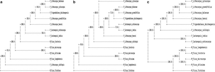
The clusterings of the 13 tree species with dissimilarity measures, from left to right d₂(a), , and with k = 9 using all the reads. The number on each internal branch is the fraction of times the branch occurs in 100 random sampling using γ = 5% of the reads.

Second, in order to see whether the clustering of the tree species can be correctly inferred using only a portion of the shotgun read data, we use γ = 5% of the total read data for each tree species to cluster them. Since the γ percent of the reads can be sampled randomly from the original read data, the resulting clustering of the tree species can be different. To study the variation of the clusters due to random sampling of the reads, we repeat the sampling process of the reads 100 times and calculate the frequencies of each internal branch of the clustering using all the reads occurring among the 100 clusterings. The frequencies are given in Figure 4 for k = 9 and γ = 5%.

It can be seen from the figure that the two groups of tree species can be completely separated using the dissimilarity measures and for any k = 7, 9, 11. However, the tree species cannot be distinguished using the dissimilarity measure d₂. These two tree groups are quite far apart, as they are in different orders and probably separated by at least 50 million years, if not considerably longer (Cannon, personal communication). A good clustering should be able to separate the two groups of trees. This result indicates that and are more sensitive to distinguish the tree species than d₂. With , most of the resulting clusters can be completely recovered with only 5% of the reads. However, the clustering with is less stable when a small fraction of the data are available.

In addition, Ficus altissima and Ficus microcarpa cluster together using all three dissimilarity measures, which is consistent with the fact that both are large trees and are closely related while the other three Moraceae species are small dioecious shrubs. Similarly, the two Castanopsis species within the Fagaceae group also cluster together separate from the others using . Thus, the clustering based on is the most reasonable among the three dissimilarity measures we study. Finally, we note that the clustering by is not perfect. F. Trigonobalanus is an ancestral genus that is very divergent from the rest of the family and has undergone considerable sequence evolution. It should not group within Lithocarpus (Cannon, personal communication).

4. Discussion

We modified the original D₂, , and statistics for alignment-free sequence comparison of two long sequences to the scenario of genome sequence comparison using NGS data. Based on the HMM model for long sequences with random instances of motif occurrences (Reinert et al., 2009; Wan et al., 2010; Zhai et al., 2010) and a general model for the sampling of NGS reads from the genome, we studied the approximate distributions of D₂, , and . We also studied the power of detecting the relationships between two sequences related through the common motif model by both simulations and theoretical studies, and studied factors affecting the power of these statistics including genome sequence length, coverage of the NGS reads, read length, word length, and the distribution of the reads along the genome sequence. It is shown that and are more powerful than D₂ for detecting relationships between two sequences related through a common motif model. These results are consistent with those for alignment-free comparison of long sequences found in Reinert et al. (2009) and Wan et al. (2010). We also found that and are generally less powerful when applied to NGS data than when they are applied to complete sequences. Heterogeneity in the sampling of reads along the genome further decreases the power of these statistics. On the other hand, when the sampling of reads is relatively homogeneous across the genome and the coverage is high, the power of and approaches the power that is achieved when these statistics are applied to complete sequences. Based on these statistics, we defined corresponding dissimilarity measures d₂, , and with ranges from 0 to 1. We applied the dissimilarity measures with some modifications to cluster five mammalian species and showed that they can all cluster them well when the tuple size is 9 or 11. When applied to the real shotgun read data from 13 tree species whose complete genome sequences are unknown, the and dissimilarity measures can correctly separate the two groups of tree species even with 5% of the reads from the shotgun read data sets.

Although we showed the usefulness of and for detecting the relationships between sequences and for clustering sequences using NGS data without assembly, our study has several limitations. First, we assumed that the background sequences are iid, which can be violated for many real molecular sequences. One solution is to use the Markov model to fit the background sequences. In this case, the D₂, , and should be further modified by replacing p_w with the probability of word pattern w according to the Markov model. We expect that the qualitative results regarding the relationships among D₂, , and will still hold. Second, we assumed that the foreground consists of just one motif. In many regulatory sequences, the regulatory modules consist of multiple motifs. Simulation studies can be carried out to compare the performance of the different statistics under the module assumption. However, theoretical formulas for calculating the power of the statistics can be challenging. Third, in modeling the distribution of the shotgun reads from NGS, although we considered heterogeneous distribution of the reads along the genome, we did not assume that the sampling probabilities λ_i depend on the base compositions at the neighborhood of position i. Previous studies (Hansen et al., 2010; Li et al., 2010) showed that the sampling probabilities are associated with the base composition in the neighborhood of the position. One solution to this problem is to ignore the first 6–10 bases of the reads and only consider the remaining bases of the reads. Without trimming each read, the k-tuple composition vector from the shotgun read data may be significantly different from the k-tuple composition from the original genome that the shotgun read data are sampled from. On the other hand, new sequencing technologies will reduce the dependence of sampling probability on the base composition and the read distributions will be increasingly homogeneous. Despite all these problems, we expect that our study lays the foundations for the study of alignment-free sequence comparison based on NGS shotgun read data.

Acknowledgments

The research is supported by National Natural Science Foundation of China (No.10871009; 10721403; 60928007; 31171262; 11021463), National Key Basic Research Project of China (No.2009CB918503), and Graduate Independent Innovation Foundation of Shandong University (GIIFSDU) (ZYZ). FS is partially supported by US NIH P50 HG 002790 and R21HG006199; and NSF DMS-1043075 and OCE 1136818. We sincerely thank Professors Michael S. Waterman and Gesine Reinert for collaborations and constant discussion on the development of alignment-free sequence comparison. The article would have been impossible without their deep insights into the statistics for alignment-free sequence comparison. We also thank Professor Chuck Cannon for his insightful comments on the evolutionary relationships of the 13 tree species, and Mr. Michael Klein for carefully reading the article and giving valuable suggestions.

Disclosure Statement

The authors declare that no competing financial interests exist.

References

- Blaisdell B.E. A measure of the similarity of sets of sequences not requiring sequence alignment. Proc. Natl. Acad. Sci. U.S.A. 1986;83:5155–5159. doi: 10.1073/pnas.83.14.5155. [DOI] [PMC free article] [PubMed] [Google Scholar]
- Cannon C.H. Kua C.S. Zhang D. Harting J.R. Assembly free comparative genomics of short-read sequence data discovers the needles in the haystack. Mol. Ecol. 2010;19((Suppl. 1)):146–160. doi: 10.1111/j.1365-294X.2009.04484.x. [DOI] [PubMed] [Google Scholar]
- Domazet-Lošo M. Haubold B. Alignment-free detection of local similarity among viral and bacterial genomes. Bioinformatics. 2011;27:1466–1472. doi: 10.1093/bioinformatics/btr176. [DOI] [PubMed] [Google Scholar]
- Hansen K.D. Brenner S.E. Dudoit S. Biases in Illumina transcriptome sequencing caused by random hexamer priming. Nucleic Acids Res. 2010;38:e131. doi: 10.1093/nar/gkq224. [DOI] [PMC free article] [PubMed] [Google Scholar]
- Ivan A. Halfon M. Sinha S. Computational discovery of cis-regulatory modules in Drosophila without prior knowledge of motifs. Genome Biol. 2008;9((1)):R22. doi: 10.1186/gb-2008-9-1-r22. [DOI] [PMC free article] [PubMed] [Google Scholar]
- Jun S.R. Sims G.E. Wu G.A. Kim S.H. Whole-proteome phylogeny of prokaryotes by feature frequency profiles: An alignment-free method with optimal feature resolution. Proc. Natl. Acad. Sci. U.S.A. 2010;107((1)):133–138. doi: 10.1073/pnas.0913033107. [DOI] [PMC free article] [PubMed] [Google Scholar]
- Leung G. Eisen M.B. Identifying CIS-regulatory sequences by word profile similarity. PLoS One. 2009;4:e6901. doi: 10.1371/journal.pone.0006901. [DOI] [PMC free article] [PubMed] [Google Scholar]
- Li J. Jiang H. Wong W.H. Modeling non-uniformity in short-read rates in RNA-Seq data. Genome Biol. 2010;11:R50. doi: 10.1186/gb-2010-11-5-r50. [DOI] [PMC free article] [PubMed] [Google Scholar]
- Lippert R.A. Huang H.Y. Waterman M.S. Distributional regimes for the number of k-word matches between two random sequences. Proc. Natl. Acad. Sci. U.S.A. 2002;100:13980–13989. doi: 10.1073/pnas.202468099. [DOI] [PMC free article] [PubMed] [Google Scholar]
- Liu X. Wan L. Li J., et al. New powerful statistics for alignment-free sequence comparison under a pattern transfer model. J. Theor. Biol. 2011;284:106–116. doi: 10.1016/j.jtbi.2011.06.020. [DOI] [PMC free article] [PubMed] [Google Scholar]
- Miller W. Rosenbloom K. Hardison R.C., et al. 28-way vertebrate alignment and conservation track in the UCSC Genome Browser. Genome Res. 2007;17:1797–1808. doi: 10.1101/gr.6761107. [DOI] [PMC free article] [PubMed] [Google Scholar]
- Reinert G. Chew D. Sun F.Z. Waterman M.S. Alignment-free sequence comparison (I): statistics and power. J. Comp. Biol. 2009;16:1615–1634. doi: 10.1089/cmb.2009.0198. [DOI] [PMC free article] [PubMed] [Google Scholar]
- Richter D.C. Ott F. Auch A.F., et al. MetaSim: a sequencing simulator for genomics and metagenomics. PLoS One. 2008;3:e3373. doi: 10.1371/journal.pone.0003373. [DOI] [PMC free article] [PubMed] [Google Scholar]
- Sims G.E. Jun S.R. Wu G.A. Kim S.H. Alignment-free genome comparison with feature frequency profiles (FFP) and optimal resolutions. Proc. Natl. Acad. Sci. U.S.A. 2009;108:2677–2682. doi: 10.1073/pnas.0813249106. [DOI] [PMC free article] [PubMed] [Google Scholar]
- Vinga S. Almeida J. Alignment-free sequence comparison-a review. Bioinformatics. 2003;19:513–523. doi: 10.1093/bioinformatics/btg005. [DOI] [PubMed] [Google Scholar]
- Wan L. Reinert G. Sun F. Waterman M.S. Alignment-free sequence comparison (II): theoretical power of comparison statistics. J. Comput. Biol. 2010;17:1467–1490. doi: 10.1089/cmb.2010.0056. [DOI] [PMC free article] [PubMed] [Google Scholar]
- Zhai Z.Y. Ku S.Y. Luan Y.H., et al. The power of detecting enriched patterns: An HMM approach. J. Comput. Biol. 2010;17:581–592. doi: 10.1089/cmb.2009.0218. [DOI] [PMC free article] [PubMed] [Google Scholar]
- Zhang Z.D. Rozowsky J. Snyder M., et al. Modeling ChIP sequencing in silico with applications. PLoS Comput. Biol. 2008;4:e1000158. doi: 10.1371/journal.pcbi.1000158. [DOI] [PMC free article] [PubMed] [Google Scholar]
Associated Data
This section collects any data citations, data availability statements, or supplementary materials included in this article.