Joint Modeling, Covariate Adjustment, and Interaction: Contrasting Notions in Risk Prediction Models and Risk Prediction Performance

Abstract

Epidemiologic methods are well established for investigating the association of a predictor of interest and disease status in the presence of covariates also associated with disease. There is less consensus on how to handle covariates when the goal is to evaluate the increment in prediction performance gained by a new marker when a set of predictors already exists. We distinguish between adjusting for covariates and joint modeling of disease risk in this context. We show that adjustment versus joint modeling are distinct concepts, and we describe the specific conditions where they are the same. We also discuss the concept of interaction among variables and describe a notion of interaction that is relevant to prediction performance. We conclude with a discussion of the most appropriate methods for evaluating new biomarkers in the presence of existing predictors.

Historically, risk prediction in medicine was limited to simple models using perhaps just a single predictor such as age or family history. With the advent of genomics, proteomics, and metabalomics, we are now in an age of high-throughput biology. Corresponding to the increase in the kinds and amount of data available on patients, there is a surge of interest in predictive models. With the large numbers of potentially predictive markers that are available, risk modeling is inevitably multivariate. Therefore, one must consider the role of covariates in predictive models. However, in contrast to therapeutic and etiologic studies, concepts of covariate adjustment are not well established when the goal is evaluating classification or prediction performance.¹

This article addresses questions related to assessing the improvement in prediction performance gained by using a new biomarker to make predictions in addition to existing predictors. We call this the incremental value of the biomarker. We will make use of receiver operating curves, also known as ROC curves, to assess prediction performance, and we will use AUC to denote “area under the ROC curve.”

As a motivating example, consider the problem of evaluating the capacity of newly discovered genetic markers to improve prediction for breast cancer. Making accurate predictions is clinically important because, for example, women at low risk could be spared the expense, discomfort, stress, and risk of false positives associated with screening mammography. On the other hand, women at high risk of breast cancer are candidates for prophylactic tamoxifen therapy. However, taking tamoxifen increases risks of endometrial cancer, stroke, and pulmonary embolism, and so only women who are clearly at high risk of breast cancer should be advised to take tamoxifen for prevention.

One issue in studying any predictor of breast cancer is how to consider age. A woman’s age is very predictive of breast cancer risk. Gail² notes the fallacy in ignoring age when considering new markers for breast cancer: “Some investigators compare case patients and control subjects over large age ranges. Because age is a strong predictor of breast cancer risk and is included in all risk models and because case patients tend to be older than control subjects, doing so increases the AUC value.”

Gail² investigated whether seven common, recently identified single-nucleotide polymorphisms (SNPs) could improve breast cancer prediction over existing models. Age-matched data allowed Gail to adjust for the predictive ability of age by examining the predictive ability of the SNPs in cases and controls of approximately the same age. In other words, the strategy was to evaluate the new predictors by stratifying on the existing predictor (in this context, age). Gail’s measure of predictive ability was the area under the age-stratified ROC curves. This amounts to adjusting the ROC curve for age.¹ In contrast, Wacholder et al³ took a fundamentally different approach; they examined the classification performance of risk models that incorporated novel markers of ten genetic variants, as well as traditional risk factors, including age. The researchers calculated the ROC curve for the joint risk model and then compared it with the ROC curve for the risk model without the addition of genetic variants.

The different analytic strategies of Gail² and Wacholer et al³ raise many interesting questions. How do the AUC values for the new markers evaluated in groups that are homogeneous with respect to the existing predictors² relate to the change in the AUC by adding the new markers to an existing risk set of predictors?³ What do we learn about the value of the new marker for the overall population, which includes women of different ages? We explore these methodological questions in this paper. We then contrast traditional concepts of covariate adjustment in predictive modeling with covariate adjustment in assessing the predictive performance of a biomarker. The former entails joint prediction using an existing marker X and a new marker Y , whereas the latter evaluates the performance of Y in groups homogeneous with respect to X. We describe the very limited conditions under which the ROC curve for the joint risk model is the same as the covariate adjusted ROC curve. We then discuss the concept of interaction in the context of evaluating the predictive performance of a marker. We demonstrate that examining interaction in terms of odds ratios is not relevant to whether there is an interaction for predictive performance. Next we discuss the implications of the ideas presented for predictive modeling. We explore these ideas further in a dataset of predictors for prostate cancer and a dataset of predictors of renal artery stenosis.

Covariate Adjustment versus Joint Modeling

Consider a simplified epidemiologic study. There is a binary variable D indicating disease, a variable X known to be associated with disease, and an additional variable of interest Y . In our example, D is occurence of breast cancer within 5 years, X is age, and Y are SNPs. We might model the risk of disease using logistic regression:

$$\text{logit}P(D=1|X,Y)=\text{logit}(\mathit{\text{risk}}(X,Y))={\beta }_0+{\beta }_{1}X+{\beta }_{2}Y$$ (1)

In traditional epidemiology there are two complementary ways in which a model such as Equation (1) is interpreted. First, we can say β₂ summarizes the association between Y and the log odds of disease for subjects with the same value of X. We call this the covariate adjustment interpretation. Covariate adjustment corresponds to the concept of stratifying subjects according to a variable, in this case stratifying by X. A second interpretation is that of joint prediction – model (1) contains both X and Y is therefore a joint model for the log odds of disease using X and Y as predictors.

We therefore argue that in epidemiology the concepts of adjusting for covariates and of joint modeling are at least partially conflated because the same model can be used for both. However, for discriminating two classes of patients, cases (D = 1) and controls (D = 0), we next show that stratification and joint modeling are distinct concepts.

ROC curves are useful and popular tools for summarizing the ability of a marker or a risk score to discriminate cases and controls. For a single continuous predictor Y, ROC_Y() describes the ability of Y to discriminate between cases and controls by plotting the true positive rate P(Y > y|D = 1) against the false positive rate P(Y > y|D = 0). ROC_X,Y() refers to the ROC curve for a predictive model that uses both X and Y. For joint prediction, it is known that the optimal way to combine X and Y for discrimination is to predict disease based on risk(X,Y) ≡ P(D = 1|X,Y ).^4–6 That is, the ROC curve for the combination defined by risk(X,Y) has the best ROC curve compared with all other possible combinations of X and Y . Therefore, we write ROC_X,Y() for the ROC curve for the risk function, ROC_risk(X,Y)(). In contrast the curve ROC_Y|X() is the ROC curve for Y stratified on X. It describes the ability of Y to discriminate between cases and controls in sub-populations that are homogeneous with respect to X. When ROC_Y|X() does not depend on X, it is called the covariate-adjusted ROC curve. Gail’s analysis addresses the covariate adjusted ROC curve, ROC_Y|X(), while Wacholder et al study the joint ROC curve, ROC_X,Y().^2–3

Another way to understand the difference between ROC_X,Y() and ROC_Y|X() is to consider how they might be estimated using a tool such as model (1). To estimate ROC_X,Y(), one would take a sample of patients for which X,Y, and D are known, use model (1) to estimate risks of disease, and then estimate the ROC curve that summarizes the overlap in these estimated risks between diseased and non-diseased persons. In contrast, to estimate ROC_Y|X() one must condition on X. After fitting model (1), one would take a sample of patients with the same value of X, use model (1) to get estimated risks based on the subjects’ Y values and their shared value of X. One could then make an empirical ROC curve based on these estimated risks. Averaging over X gives the covariate adjusted ROC curve.

Despite the fact that the concepts of covariate adjustment and joint modeling are intertwined when studying associations between disease and predictors, ROC_X,Y = ROC_Y|X only in some very specific cases. We present Example 1 to provide intuition before stating a general result.

Example 1. We present an example where there are two predictors of disease, X and Y , and show that ROC_X,Y() ≠ ROC_Y|X(). In this example, X is a binary predictor. For concreteness let X represent two categories of age, say, with X=0 for younger subjects and X=1 for older subjects. Let the distribution of the new marker Y be as follows:

$$Y|(X=0,D=0)~N(0,1)Y|(X=0,D=1)~N(2,1)Y|(X=1,D=0)~N(2,1)Y|(X=1,D=1)~N(4,1)$$

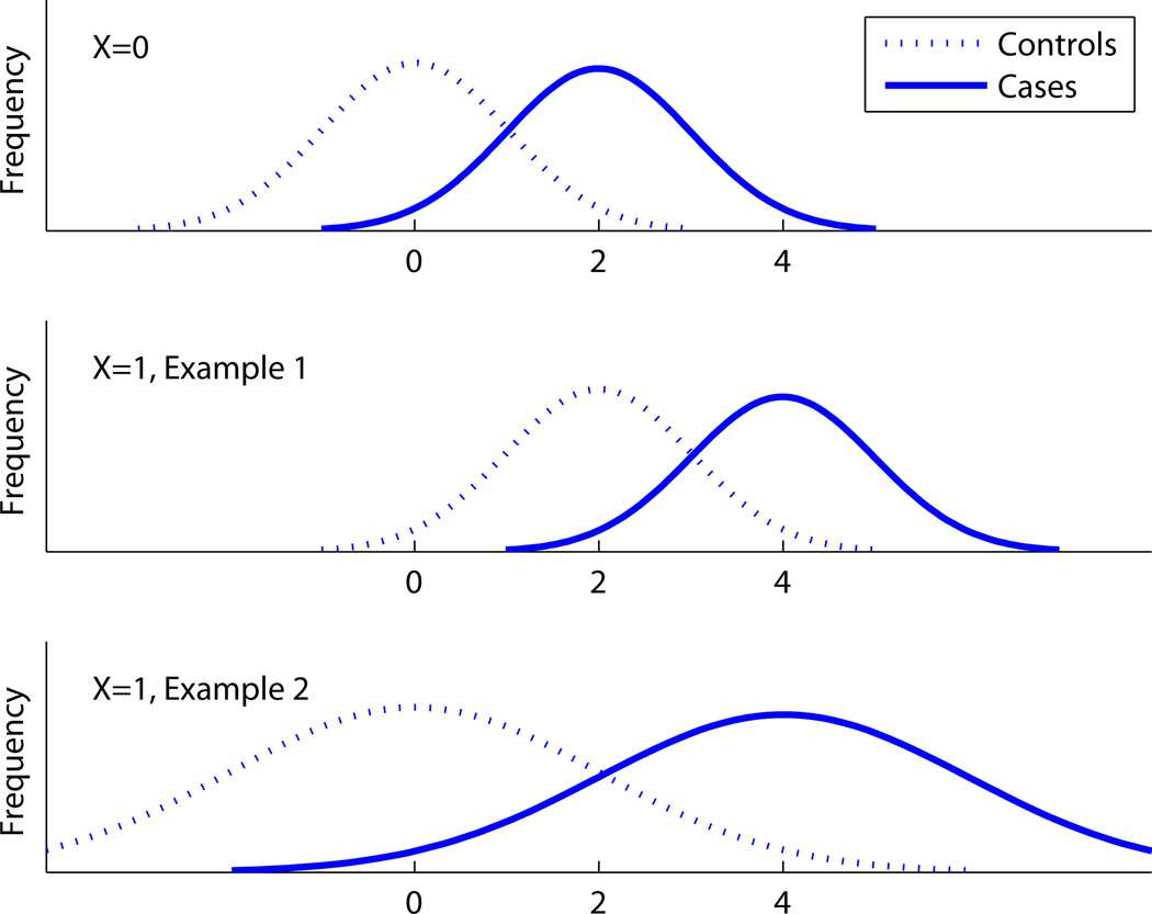
The top two panels of Figure 1 illustrate the distribution of Y. Let p₀ = P(D = 1|X = 0) and p₁ = P(D = 1|X = 1) be the prevalences of disease in the younger and older sub-populations, and let q = P(X = 1) be the proportion of subjects in the population that are in the older age category.

Figure 1.

The distribution of Y for Examples 1 and 2.

ROC_Y|X can be computed simply by conditioning on X. It is obvious that ROC_Y|X=0 = ROC_Y|X=1, which we write as AROC, because in both cases the ROC curve comes from the overlap between two unit-variance normal distributions with a difference of two in their means.

ROC_X,Y is computed from risk(X,Y) ≡ P(D = 1|X,Y). For this simple model, Bayes’ theorem gives formulas for these risks as a function of X and Y:

$$\mathit{\text{risk}}(X,Y)=\{\begin{array}{cc}\frac{p_0{e}^{-\frac{1}{2}{(Y-2)}^2}}{(1-p_0)e^{-\frac{1}{2}{Y}^2}+p_0{e}^{-\frac{1}{2}{(Y-2)}^2}},\hfill & \text{if}X=0\hfill \\ \frac{p_1{e}^{-\frac{1}{2}{(Y-4)}^2}}{(1-p_1)e^{-\frac{1}{2}{(Y-2)}^2}+p_1{e}^{-\frac{1}{2}{(Y-4)}^2}},\hfill & \text{if}X=1.\hfill \end{array}$$

It can be shown algebraically that ROC_X,Y() = ROC_Y|X() if and only if p₀ = p₁. This also follows from the general result proved in the next subsection. In other words, the ROC curve for the joint prediction is the same as the ROC curve for Y adjusted for X if and only if X is not a risk factor. If X is a risk factor (i.e. p₀ ≠ p₁), ROC_X,Y and ROC_Y|X are different curves.

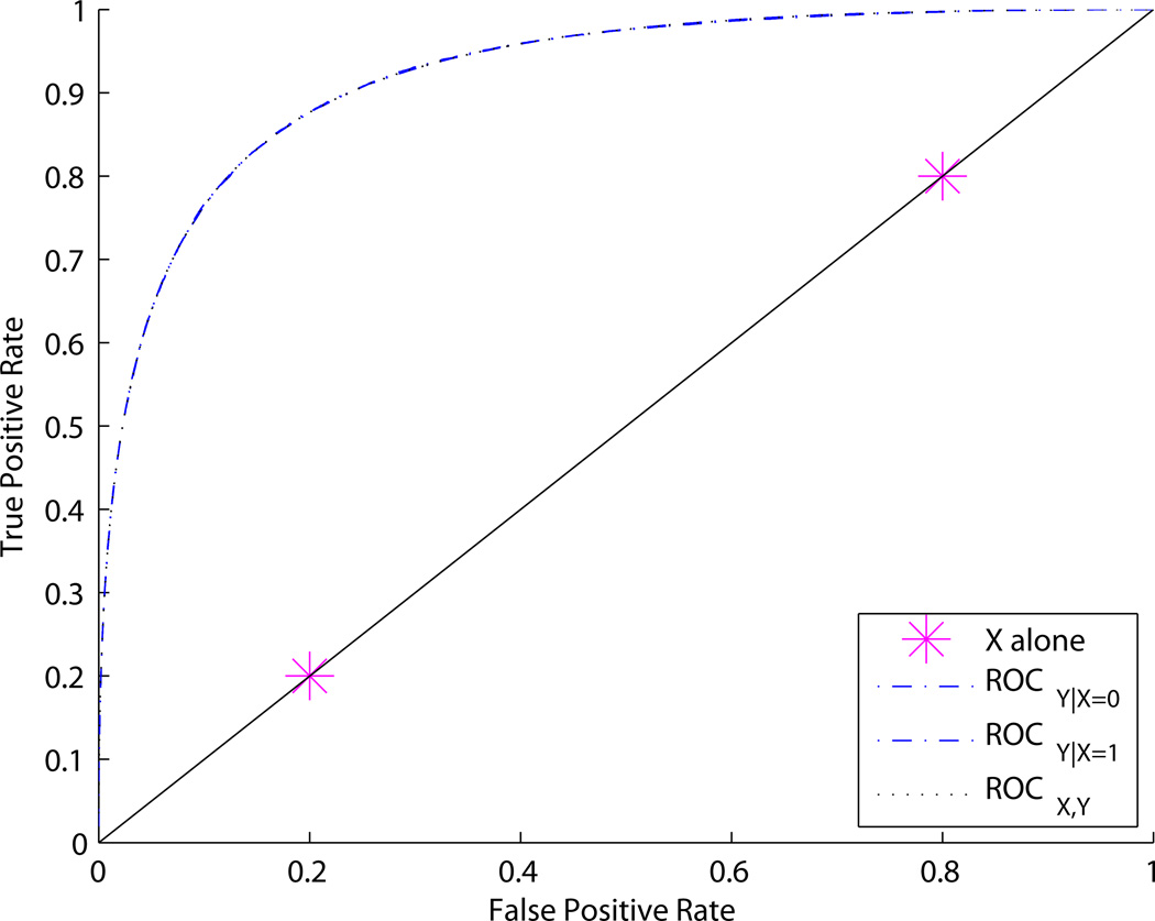
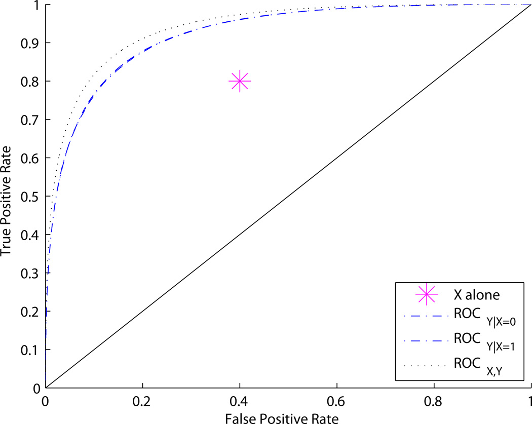
Figures 2 and 3 show adjusted and unadjusted ROC curves for different values of p₀, p₁, and q. Figure 2 shows an example where p₀ = p₁; the covariate-adjusted curves ROC_Y|X and joint ROC curve ROC_Y,X are the same. In contrast, Figure 3 shows an example where p₀ ≠ p₁. In this case ROC_Y,X > ROC_Y|X. An intuitive explanation for the difference is that, in the first example, knowing X tells us how to interpret Y, but does not provide any independent information about disease status. This is a case where we might say “X calibrates Y”. In the second example, X provides independent information about disease status in addition to telling us how to interpret Y.

Figure 2.

ROC curves for Example 1. ROC_X,Y = ROC_Y|X whenever p₀ = p₁, regardless of q. In this figure, p₀ = p₁ = 0.1, q = 0.2.

Figure 3.

ROC curves for Example 1. ROC_X,Y > ROC_Y|X whenever p₀ ≠ p₁. In this figure, p₀ = 0.4, p₁ = 0.1, q = 0.5.

A General Result about ROC_X,Y and ROC_Y|X. The next result shows that in order for the joint and covariate adjusted ROC curves to be equal, X cannot be informative of disease status marginally. Moreover, the role of X in the joint risk model can at most be to calibrate Y. In particular, we let W = F_D̄,X(Y), where F_D̄,x is the cumulative distribution of Y in the population of controls with X = x. Huang and Pepe⁷ use the term “covariate-specific percentile value” for 100 × W, which refers to the fact that Y is transformed to a percentile according to the distribution of Y in the reference population with D = 0 and X = x. Recall that we use the notion of a covariate-adjusted ROC curve when the conditional (or stratified) ROC curves, ROC_Y|X() are the same across X values (or strata). In this setting we have the following result.

Result 1. Let ROC_Y|X be the same for all X. Then we have the following equivalences.

$$RO{C}_{X,Y}(·)=RO{C}_{Y|X}(·)$$ (2)

$$\iff P(D=1|X,Y)=P(D=1|W)$$ (3)

$$\iff P(D=1|X)=P(D=1)$$ (4)

Proof of Result 1. We prove the result for continuous Y with common support for Y in case and control populations. Janes and Pepe⁸ showed that the covariate-adjusted ROC curve is the same as the ROC curve for W, written ROC_W(). Also, because F_D̄,X() is a strictly increasing function, P(D = 1|X,Y) = P(D = 1|X,W), and therefore the ROC curve for (X,Y) is the same as that for (X,W). We therefore rewrite (2) as

$$RO{C}_{X,W}(·)=RO{C}_W(·).$$ (5)

By the lemma in the Appendix, (5) implies that

$$P(D=1|X,W)=P(D=1|W)$$

and therefore (3) holds. In the reverse direction it is obvious that (3) implies (5), which is equivalent to (2).

Bayes’ theorem yields the identity

$$\text{logit}P(D=1|X,W)=\text{logit}P(D=1|X)+\text{log}\frac{f(W|D=1,X)}{f(W|D=0,X)},$$ (6)

where f denotes the probability density of W. The distribution of W conditional on X is uniform (0,1) in controls. So, f(W|D = 0,X) does not depend on X. Neither does f(W|D = 1,X) depend on X because, according to Janes and Pepe,⁸ the cumulative distribution of 1 − W given D = 1 and X is the covariate-adjusted ROC curve, which we have assumed does not depend on X. Therefore, neither f(W|D = 1,X) nor f(W|D = 0,X) depend on X. It follows that if P(D = 1|X,W) does not depend on X, then neither does P(D = 1|X), and vice versa. In other words, (3) holds if and only if (4) holds.

We emphasize that if X is not useful for prediction marginally, it may still have a role in a joint risk model. In particular, X will be useful if X calibrates Y . Example 1 demonstrates this phenomenon. The equivalence between (3) and (4) under the assumption that there is a single stratified ROC curve states this formally and appears to be a new, general, and interesting result.

Corollary 1. Let ROC_Y|X be the same for all X and suppose P(D = 1|X) ≠ P(D = 1) for some X. Then ROC_X,Y(·) ≥ ROC_Y|X(·).

Proof of Corollary 1. As mentioned in the proof of Result 1, ROC_Y|X(·) = ROC_W(·) where W = F_D̄,X(Y).⁸ On the other hand, ROC_X,Y(·) ≡ ROC_risk(X,Y)(·) is known to be the optimal combination of X and Y for predicting disease: for a given false-positive rate f, ROC_X,Y(f) dominates any other combination of X and Y for predicting D.^4–6 This implies ROC_X,Y(·) ≥ ROC_W(·), because W refers to a particular way of combining X and Y.

Concepts of Interactions among Predictors

In any context in which a statistical model is used with multiple predictors, the possibility of interactions among predictors can arise. What precisely one means when one says that two variables “interact” depends on the context, and the most appropriate definition of “interaction” is always context-dependent.⁹ For many researchers who work in epidemiology and often use logistic regression models, the phrase “X and Y interact” means that the odds ratio for Y depends on X (OR_Y|X varies with X). However, this is not the most appropriate definition of interaction when discriminating between cases and controls. Rather, a more relevant notion of interaction is to say that X and Y interact if ROC_Y|X varies with X. Examples 2 and 3 in this section demonstrate that these notions of interaction are not the same.

Example 2: OR_Y|X depends on X; ROC_Y|X does not. Consider the following variation on the data model in Example 1. When X = 0 the distribution of Y is exactly the same as Example 1. The bottom panel of Figure 1 shows the distribution of Y when X = 1.

$$Y|(X=0,D=0)~N(0,1)Y|(X=0,D=1)~N(2,1)Y|(X=1,D=0)~N(0,2)Y|(X=1,D=1)~N(4,2)$$

ROC_Y|X is the same as in Example 1 and, in particular, does not depend on X: ROC_Y|X=0 = ROC_Y|X=1. Note that for X = 1 the larger separation in the means of the distribution of Y for cases and controls is exactly compensated for by the larger variability.^10,p.82

However, the odds ratios do depend on X in this example. To see this, we use Bayes’ theorem to calculate

• logitP(D = 1|Y,X = 0) = 2Y − 2 + logit(p₀), so OR_Y|X=0 = exp(2) while

• logitP(D = 1|Y,X = 1) = Y − 2 + logit(p₁), so OR_Y|X=1 = exp(1).

Observe in this example that, according to Result 1, if X is not marginally predictive then the role of X in the risk model is only to calibrate Y . However, if X is marginally predictive of D then the joint model will involve additional effects of X on risk and the ROC curve for the joint risk model will be higher than that of the common stratified ROC curve.

Example 3: ROC_Y|X depends on X; OR_Y|X does not. Let X have a Bernoulli distribution with $P(X=1)=P(X=0)=\frac{1}{2}$. Let Y ~ N(X,1). Let the risk of disease follow a logistic model:

$$\text{logit}P(D=1|X,Y)=X+2Y$$ (7)

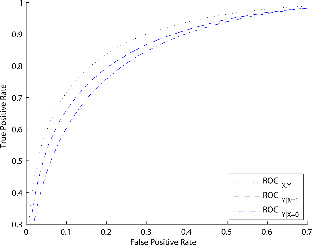
We simulated X and Y values, used model (7) to calculate risks of disease, and simulated disease status based on these risks. Figure 4 shows ROC_X,Y and ROC_Y|X. Note that ROC_Y|X=0 ≠ ROC_Y|X=1. Model (7) makes it obvious that OR_Y|X does not depend on X.

Figure 4.

ROC curves for Example 3. ROC_Y|X can depend on X in some settings where OR_Y|X does not depend on X.

Implications for Predictive Models

Result 1 says that ROC_X,Y() and ROC_Y|X() are distinct curves except under special circumstances. Therefore, one should use the curve appropriate to the task at hand.

One type of application is when the new marker Y is envisioned to be used in conjunction with X in the entire population for which prediction is performed. In such a setting, ROC_X,Y() is the appropriate curve to consider and should be compared with ROC_X(). ROC_Y|X() should not be used for this purpose. A limited exception to this conclusion is that ROC_Y|X() can be used to test the null hypothesis that the incremental value of Y is 0. This is because ROC_Y|X() differs from the 45-degree line if and only if ROC_X,Y() > ROC_X().¹¹ However, hypothesis testing is of questionable value because the real challenge is to identify markers that improve prediction by a clinically useful amount.

In other situations, ROC_Y|X() may be the curve of interest. Suppose X is considered to define clinically distinct sub-groups of the population, or X can clearly define a small proportion of the population as very high (or low) risk. Researchers may envision that the new marker Y will be used differently in different sub-populations, or will be used only in certain sub-populations defined by X. Consider the breast cancer example, and suppose X indicates whether a subject has a mutation in certain genes BRCA1 or BRCA2. In this case, X identifies a small proportion of women at much higher risk of breast cancer, and one may wish to consider the predictive ability of a marker Y separately in the two groups defined by X.

In the previous section we distinguished two notions of interaction: OR_Y|X depends on X vs. ROC_Y|X depends on X. What are the implications of this distinction for predictive modeling? Suppose risks are estimated with a regression model and one finds evidence to support an interaction term in the model. Returning to Example 2, the true risk model can be written:

$$\text{logit}P(D=1|X,Y)=\text{logit}(p_0)-2+(\text{logit}(p_1)-\text{logit}(p_0))X+2Y-X·Y$$ (8)

In other words, on the logit scale the risks are a linear combination of X, Y , and X · Y. We emphasize that it is appropriate (and potentially important) to include the interaction term in modeling the risks. The point is simply that, just because there is an interaction term in the regression model, this does not mean that Y has different predictive capacity in the sub-populations defined by X. Furthermore, an example in the next section shows that a large interaction in terms of odds ratios can have no impact on discriminating between cases and controls.

Application to Prostate Cancer and Renal Artery Stenosis

In this section we examine real data to illustrate some of the ideas discussed in this paper. The first dataset is from a prospective study of 557 men scheduled for prostate biopsy reported by Deras and colleagues.¹² Thirty-five percent of men had a positive biopsy. The second dataset is from a study of 426 subjects, first reported by Janssens and colleagues,¹³ wherein 23% had the outcome, stenosis of the renal artery. Both datasets contain multiple predictors, but to illustrate the ideas we will limit ourselves to two predictors at a time. Our intent is to illustrate key concepts and so we will not be concerned with statistical significance.

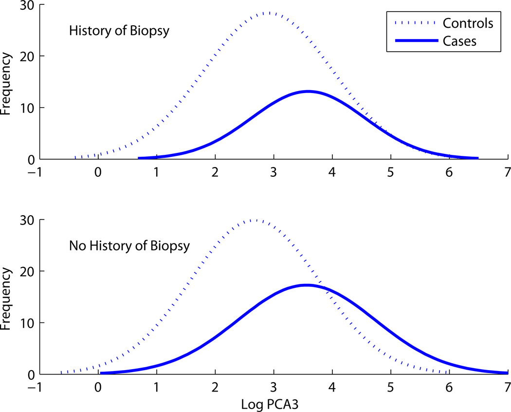
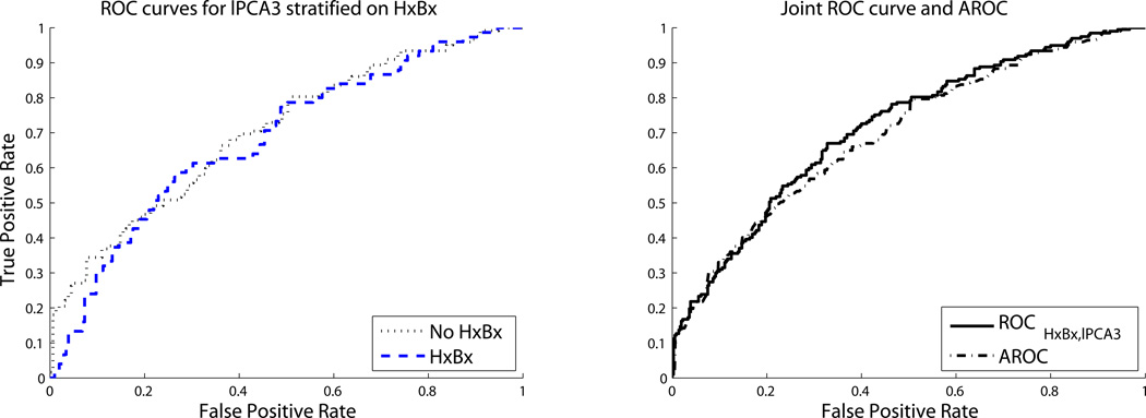
In the prostate cancer dataset, we consider the binary variable indicating whether a man has a history of previous biopsy (HxBx) and the continuous variable lPCA3, which is the expression of a particular gene, PCA3, on the log scale. HxBx is predictive on its own, with a diagnosis of cancer in 44% of those without a history of biopsy and 27% of those with a previous prostate biopsy. Figure 5 suggests that the predictive ability of lPCA3 is very similar in men with and without a history of biopsy for prostate cancer; this observation is confirmed by the ROC curves for lPCA3 stratified on HxBx (left panel of Figure 6). Corollary 1 above says that ROC_HxBx,lPCA3 should be greater than ROC_lPC3|HxBx because HxBx is marginally predictive. The right panel of Figure 6 shows that this is approximately the case, because the joint ROC curve for HxBx and lPCA3 dominates the AROC, except at small false-positive rates, where the densities show lPCA3 is a better predictor for men without history of biopsy. The joint risks of prostate cancer using HxBx and lPCA3 were estimated using an additive logistic regression model. The fact that ROC_HxBx,lPCA3 is not strictly greater than ROC_lPC3|HxBx does not contradict the theoretical result, but rather reflects the fact that the fitted model is an approximation of the true risk function.

Figure 5.

The distribution of Log PCA3 among cases and controls for subjects with and without a history of biopsy.

Figure 6.

Prediction Using History of Biopsy (HxBx) and log expression of PCA3 (lPCA3).

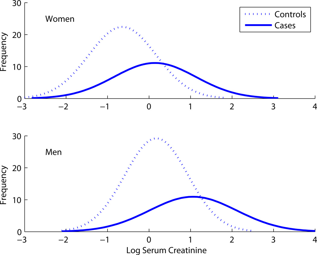
In the renal artery stenosis data, suppose that sex and log serum creatinine (lSCr) are the candidate predictors. The sex variable on its own is essentially useless as a predictor because the prevalence of renal artery stenosis in men and women is almost identical (24% in women and 22% in men). However, Figure 7 suggests that sex will be a useful predictor in combination with lSCr because a subject’s sex helps one interpret the lSCr measurement. Indeed, if we use lSCr by itself, we can discriminate cases and controls with an AUC of 0.71. We modeled risk of renal artery stenosis with logistic regression using an additive model and both lSCR and sex as predictors. Using the joint model, the AUC increases to 0.75. This illustrates another idea presented in the second section above – that a variable with no predictive capacity on its own can still be useful in a joint prediction model.

Figure 7.

Distribution of log serum creatinine for men and women, cases and controls.

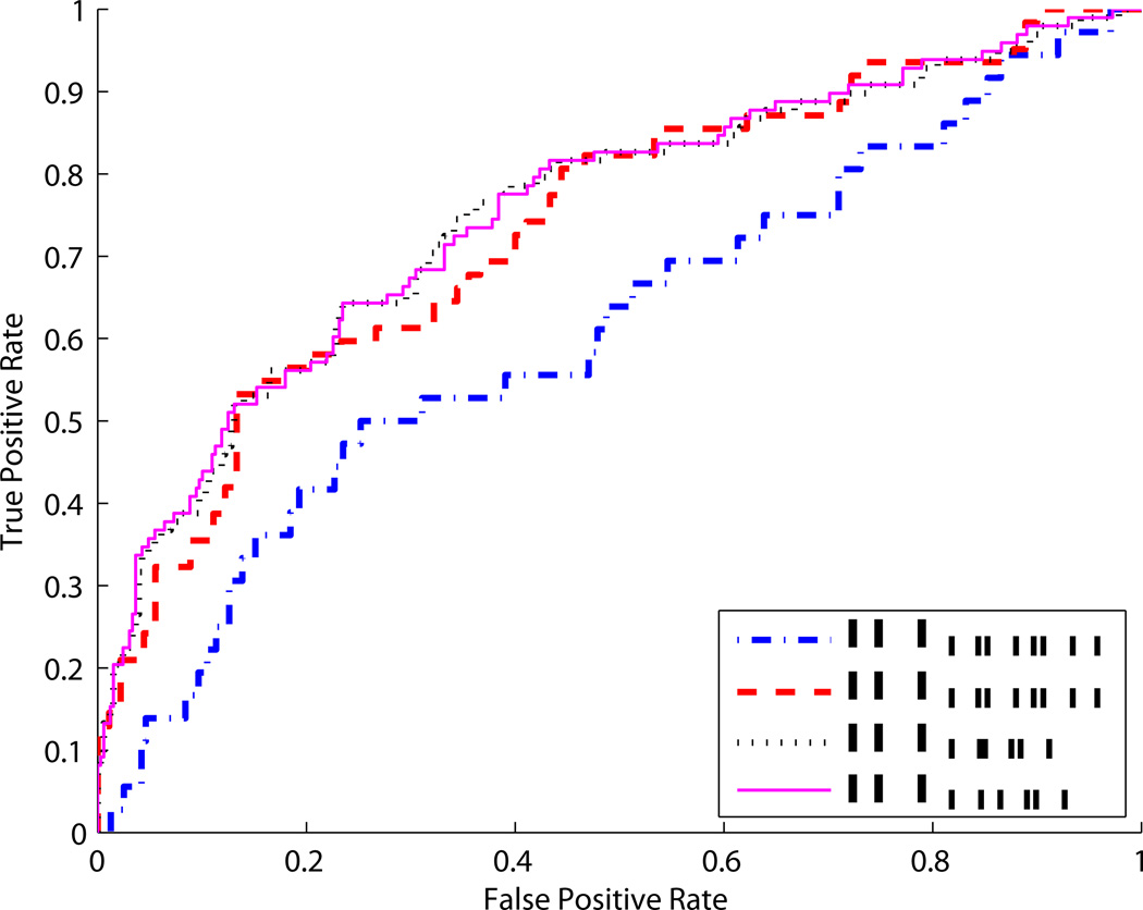
Another interesting example is to consider lSCr along with the binary predictor indicating whether a patient has vascular disease (V). If we consider lSCr as a predictor in patients with and without vascular disease, the predictive capacity is clearly different, with an AUC of 0.73 in patients with vascular disease and an AUC of 0.61 in patients without vascular disease (Figure 8). In this sense, there is an interaction between lSCr and V for discriminating cases from controls. If we consider a logistic regression model, the interaction term is substantial:

$$\text{logit}(D|V,lSCr)=-1.84+1.03V+0.41lSCr+0.55V*lSCr.$$ (9)

The odds ratio for lSCr in patients without vascular disease is 1.50 (OR_lSCr|V=0 = 1.50); in patients with vascular disease the odds ratio is 2.62 (OR_lSCr|V=1 = 2.62). Here, there are interactions both in the risk model and in the performance of the marker. Interestingly, although one might suspect that including the interaction term when modeling risks will improve prediction performance, in fact it has very little impact. Figure 8 shows that the AUC for a joint model without interaction is 0.752 while including an interaction increases it only to 0.755.

Figure 8.

ROC curves where V indicates vascular disease and lSCr is log serum creatinine. ROC_V,lSCr is based on estimating risks using logistic regression without an interaction term; ROC_V*lSCr is based on estimating risks using logistic regression with an interaction term as in Equation (9)

Discussion

We have discussed covariate adjustment, joint modelling, and interaction in the context of evaluating biomarkers for prediction and classification. First, we clarified the difference between incorporating a new predictor in a risk model that already includes established predictors, and eliminating the effect of existing predictors by adjusting for them. In particular, ROC curves for a risk model that incorporates a new predictor with existing predictors are almost never the same as ROC curves for the new predictor adjusted for existing predictors. These are equal only when the covariate has no marginal association with disease. This contrasts with the notion that covariate adjustment and joint modelling can be handled within the framework of a single risk model. Second, we contrasted notions of interaction in a classical epidemiologic context and in the context of assessing predictive performance. In epidemiology, Y and X are usually said to interact if there is evidence that OR_Y|X varies with X. In prediction performance assessment, a more relevant notion of interaction is whether ROC_Y|X varies with X. We demonstrated that these notions of interaction are distinct.

Note that ROC regression methods can be used to assess the evidence that the predictive capacity of a marker Y varies with a covariate X.¹⁴ These methods also provide a way to evaluate the assumption of a single adjusted ROC curve. For example, Janes, Longton, and Pepe¹⁵ model

$${\mathrm{\Phi }}^{-1}(RO{C}_{Y|X}(f))={\alpha }_0+{\alpha }_1{\mathrm{\Phi }}^{-1}(f)+{\alpha }_{2}X$$ (10)

where f is the false-positive rate axis and ROC_Y|X(f) is the corresponding true-positive rate. They test whether α₂ = 0. Software to implement ROC regression methods is readily available¹⁵. (See the paper by Cai and Pepe¹⁶ for more general semi-parametric modeling techniques.)

Questions of study design warrant particular attention because study design determines what the data are useful for. An especially important issue in study design is matching. Typically, when cases and controls are matched on an existing predictor X, then the incremental value of Y cannot be assessed because we cannot derive P(D = 1|X,Y) and consequently cannot estimate ROC_X,Y(·).¹⁷ Therefore, matched data present additional challenges and, as always, investigators should give serious consideration before choosing a matched design.

While we have focused on ROC curves as a convenient framework for discussion, we do not mean to imply that ROC curves are the only useful summary of a risk model, or even the most important summary. Different metrics and summaries have different merits, and the most appropriate metrics depend on the context.^18–21

Appendix: Lemma for Result 1

Lemma: ROC_X,Y(·) = ROC_X(·) ⇔ P(D = 1|X,Y) = P(D = 1|X) with probability 1.

Proof: We need to prove the lemma only in the forward direction as the other direction is obvious. We first note that ROC_X,Y(·) = ROC_X(·) implies that the distribution of risk(X,Y) is equal to the distribution of risk(X). This holds because the distributions of risk(X,Y) and risk(X) are also known as the predictiveness cures for risk(X,Y) and risk(X), and it was shown by Huang and Pepe? that a predictiveness curve can be written in terms of the corresponding ROC curve and the prevalence. Equality of ROC curves therefore implies equality of predictiveness curves. It follows that var(risk(X,Y)) = var(risk(X)) and E(risk(X,Y)) = E(risk(X)). Moreover, because E[risk(X,Y)|X] = risk(X), we have E(risk(X,Y)risk(X)) = E(risk(X))². Now consider

$$E{[\mathit{\text{risk}}(X,Y)-\mathit{\text{risk}}(X)]}^2=E{(\mathit{\text{risk}}(X,Y))}^2+E{(\mathit{\text{risk}}(X))}^2-2E[\mathit{\text{risk}}(X,Y)\mathit{\text{risk}}(X)]=E{(\mathit{\text{risk}}(X,Y))}^2-E{(\mathit{\text{risk}}(X))}^2=\text{var}(\mathit{\text{risk}}(X,Y))-\text{var}(\mathit{\text{risk}}(X))=0$$

which implies that

$$\mathit{\text{risk}}(X,Y)=\mathit{\text{risk}}(X)$$ (11)

with probability 1.

REFERENCES

- 1.Janes H, Pepe MS. Adjusting for covariates in studies of diagnostic, screening, or prognostic markers: An old concept in a new setting. Am J Epidemiol. 2008;168:89–97. doi: 10.1093/aje/kwn099. [DOI] [PubMed] [Google Scholar]
- 2.Gail MH. Discriminatory accuracy from single-nucleotide polymorphisms in models to predict breast cancer risk. J Natl Cancer Inst. 2008;100:1037–1041. doi: 10.1093/jnci/djn180. [DOI] [PMC free article] [PubMed] [Google Scholar]
- 3.Wacholder S, Hartge P, Prentice R, et al. Performance of common genetic variants in breast-cancer risk models. N Engl J Med. 2010;362:986–993. doi: 10.1056/NEJMoa0907727. [DOI] [PMC free article] [PubMed] [Google Scholar]
- 4.Green DM, Swets J. Signal Detection Theory and Psychophysics. New York: Wiley; 1966. [Google Scholar]
- 5.Egan JP. Signal Detection Theory and ROC Analysis. New York: Academic Press; 1975. [Google Scholar]
- 6.McIntosh MW, Pepe MS. Combining several screening tests: Optimality of the risk score. Biometrics. 2002;58 doi: 10.1111/j.0006-341x.2002.00657.x. 657664. [DOI] [PubMed] [Google Scholar]
- 7.Huang Y, Pepe MS. Biomarker evaluation and comparison using the controls as a reference population. Biostatistics. 2009;10:228–244. doi: 10.1093/biostatistics/kxn029. [DOI] [PMC free article] [PubMed] [Google Scholar]
- 8.Janes H, Pepe MS. Adjusting for covariate effects on classification accuracy using the covariate-adjusted receiver operating characteristic curve. Biometrika. 2009;96:371–382. doi: 10.1093/biomet/asp002. [DOI] [PMC free article] [PubMed] [Google Scholar]
- 9.McKnight B. Effect modification. In: Armitage P, Colton T, editors. Encyclopedia of Biostatistics. John Wiley and Sons; 1998. [Google Scholar]
- 10.Pepe MS. The Statistical Evaluation of Medical Tests for Classification and Prediction. Oxford University Press; 2003. [Google Scholar]
- 11.Pepe MS, Kerr KF, Longton G, Wang Z. Testing for improvement in prediction model performance. Technical Report 379. 2011 doi: 10.1002/sim.5727. www.bepress.com/uwbiostat/paper379. [DOI] [PMC free article] [PubMed]
- 12.Deras IL, Aubin SMJ, Blase A, et al. PCA3 - a molecular urine assay for predicting prostate biopsy outcome. 2010. Submitted. [DOI] [PubMed] [Google Scholar]
- 13.Janssens ACJW, Deng Y, Borsboom GJ, Eijkemans MJ, Habbema JDF, Steyerberg EW. A new logistic regression approach for the evaluation of diagnostic test results. Med Decis Making. 2005;25:168–177. doi: 10.1177/0272989X05275154. [DOI] [PubMed] [Google Scholar]
- 14.Pepe MS. Three approaches to regression analysis of receiver operating characteristic curves for continuous test results. Biometrics. 2008;54 124135. [PubMed] [Google Scholar]
- 15.Janes H, Longton G, Pepe MS. Accommodating covariates in receivor operating characteristic analysis. STATA J. 2009;9:17–39. [PMC free article] [PubMed] [Google Scholar]
- 16.Cai T, Pepe MS. Semiparametric receiver operating characteristic analysis to evaluate biomarkers for disease. J Am Stat Assoc. 2002;97:1099–1107. [Google Scholar]
- 17.Janes H, Pepe MS. Matching in studies of classification accuracy: Implications for analysis, efficiency, and assessment of incremental value. Biometrics. 2008;64:1–9. doi: 10.1111/j.1541-0420.2007.00823.x. [DOI] [PubMed] [Google Scholar]
- 18.Gail MH, Pfeiffer RM. On criteria for evaluating models of absolute risk. Biostatistics. 2005;6:227–239. doi: 10.1093/biostatistics/kxi005. [DOI] [PubMed] [Google Scholar]
- 19.Pepe MS, Feng Z, Huang Y, et al. Integrating the predictiveness of a marker with its performance as a classifier. Am J Epidemiol. 2008;167:362–368. doi: 10.1093/aje/kwm305. [DOI] [PMC free article] [PubMed] [Google Scholar]
- 20.Gu W, Pepe MS. Measures to summarize and compare the predictive capacity of markers. Int J Biostatistics. 2009;5 doi: 10.2202/1557-4679.1188. Article 27. [DOI] [PMC free article] [PubMed] [Google Scholar]
- 21.Pepe M, Gu J, Morris DE. The potential of genes and other markers to inform about risk. Cancer Epidemiol Biomarkers Prev. 2010;19:655–665. doi: 10.1158/1055-9965.EPI-09-0510. [DOI] [PMC free article] [PubMed] [Google Scholar]