Poly(A) motif prediction using spectral latent features from human DNA sequences

Abstract

Motivation: Polyadenylation is the addition of a poly(A) tail to an RNA molecule. Identifying DNA sequence motifs that signal the addition of poly(A) tails is essential to improved genome annotation and better understanding of the regulatory mechanisms and stability of mRNA.

Existing poly(A) motif predictors demonstrate that information extracted from the surrounding nucleotide sequences of candidate poly(A) motifs can differentiate true motifs from the false ones to a great extent. A variety of sophisticated features has been explored, including sequential, structural, statistical, thermodynamic and evolutionary properties. However, most of these methods involve extensive manual feature engineering, which can be time-consuming and can require in-depth domain knowledge.

Results: We propose a novel machine-learning method for poly(A) motif prediction by marrying generative learning (hidden Markov models) and discriminative learning (support vector machines). Generative learning provides a rich palette on which the uncertainty and diversity of sequence information can be handled, while discriminative learning allows the performance of the classification task to be directly optimized. Here, we used hidden Markov models for fitting the DNA sequence dynamics, and developed an efficient spectral algorithm for extracting latent variable information from these models. These spectral latent features were then fed into support vector machines to fine-tune the classification performance.

We evaluated our proposed method on a comprehensive human poly(A) dataset that consists of 14 740 samples from 12 of the most abundant variants of human poly(A) motifs. Compared with one of the previous state-of-the-art methods in the literature (the random forest model with expert-crafted features), our method reduces the average error rate, false-negative rate and false-positive rate by 26, 15 and 35%, respectively. Meanwhile, our method makes ∼30% fewer error predictions relative to the other string kernels. Furthermore, our method can be used to visualize the importance of oligomers and positions in predicting poly(A) motifs, from which we can observe a number of characteristics in the surrounding regions of true and false motifs that have not been reported before.

Availability: http://sfb.kaust.edu.sa/Pages/Software.aspx

Contact: lsong@cc.gatech.edu or xin.gao@kaust.edu.sa

Supplementary information: Supplementary data are available at Bioinformatics online.

1 INTRODUCTION

Roughly speaking, when DNA is transcribed to RNA, a string of adenine (A) nucleotides, referred to as the polyadenylation tail or the poly(A) tail, is added to the 3′-end of the primary RNA transcript. Such a process is called polyadenylation, which is a step to protect RNA stability, nuclear export and translation (Bernstein and Ross, 1989; Leung et al., 2011). A poly(A) tail is ∼10–30 nt downstream of a signaling site that consists of 6 nt, which in human cells most commonly is AAUAAA (Beaudoing et al., 2000). This signaling site is known as a poly(A) signal and the corresponding 6 nt subsequences in DNA are called poly(A) motifs. Mutations in poly(A) signals can be associated with diseases, e.g. colorectal cancer (Kim et al., 2002; Pastrello et al., 2006) and compromised immunodeficiency (Das et al., 1997; Langemeier et al., 2012).

The poly(A) signal prediction problem has been studied for decades (Proudfoot, 2011). There are two versions of the problem: predicting poly(A) signals in mRNA sequences and predicting poly(A) motifs in DNA sequences. Intuitively, the former version is much simpler than the latter one because once the mRNA sequence is given, the poly(A) tail can be identified relatively easily and we need only to search for the poly(A) signal(s) in a window of at most 30 nt upstream the poly(A) tail. In DNA, however, the presence of introns in eukaryotes and the absence of poly(A) tails make the recognition much more challenging.

A number of studies have demonstrated that information from relatively short upstream and downstream sequences of the candidate poly(A) motifs can specify the true poly(A) motifs to a great extent (Ahmed et al., 2009; Akhtar et al., 2010; Chang et al., 2011; Cheng et al., 2006; Graber et al., 1999; Ji et al., 2010; Kalkatawi et al., 2012; Legendre and Gautheret, 2003; Liu et al., 2005; Salamov and Solovyev, 1997; Tabaska and Zhang, 1999). Statistical properties of the surrounding sequences were explored in different species, such as yeast (van Helden et al., 2000), fly (Retelska et al., 2006), Arabidopsis and rice (Ji et al., 2010) and human (Chang et al., 2011; Retelska et al., 2006; Tabaska and Zhang, 1999). Although significant progress has been made to the accuracy of poly(A) motif predictors, especially in human DNA sequences, such methods are all based on using sophisticated features that require additional efforts to extract and are highly dependent on domain knowledge. We therefore ask the following question: can we use machine-learning techniques to automatically extract useful features from human DNA sequences and achieve state-of-the-art poly(A) motif classification results? If the answer to this question is yes, then we can automate this genome annotation task to a great extent and potentially speed up our understanding of the underlying biology.

Automatic feature extraction techniques have been explored in many other sequence classification problems. By far, the most successful methods are hidden Markov models (HMMs), e.g. in gene finding (Lukashin and Borodovsky, 1998; Stanke and Waack, 2003), and string kernels with support vector machines (SVM), e.g. in protein classification (Leslie et al., 2004), transcription start-site recognition (Sonnenburg et al., 2006) and splice-site prediction (Sonnenburg et al., 2007). The former methods are generative models that capture the uncertainty in data using probabilistic languages, while the latter are discriminative methods that optimize specifically for the classification results. The advantages of each class of methods have rarely been combined systematically to yield even better feature extractors.

In this article, we propose a novel method for poly(A) motif prediction by marrying generative learning (HMMs) and discriminative learning (SVMs). Generative learning provides us with a rich palette for handling the uncertainty and diversity of sequence information, while discriminative learning allows us to directly optimize performance for the classification task. Here, diversity means that for the same position in the surrounding sequence of a candidate poly(A) motif, there may be multiple subsequences indicating the class label (a true motif or a false one), and uncertainty means that each of these subsequences does not give deterministic information about the class label. In particular, we use HMMs as a probabilistic generative model for DNA sequences, and develop an efficient spectral algorithm for extracting latent variable information from these models. The HMMs model not only the diversity and uncertainty of sequence information, but also long-range dependencies between subsequences at different positions, which cannot be simultaneously captured by string kernels as is discussed in Section 2.2. The spectral latent features are then fed into support vector machines to fine-tune the classification performance.

2 RELATED WORKS

We will first review the two classes of methods, expert-crafted features and string kernels, for addressing the poly(A) motif classification problem.

2.1 Features based on domain knowledge

Bioinformatics experts can craft highly informative features based on prior knowledge of the biology and physics of DNA sequences. The drawback of using these features is that they require extensive expert domain knowledge for their design as well as additional efforts to extract them.

Salamov and Solovyev developed POLYAH (Salamov and Solovyev, 1997), a tool that used a linear discriminant function-based classifier to extract features from 100 nt upstream and 200 nt downstream of a candidate poly(A) motif. Later on, polyadq was developed based on quadratic discriminant functions by encoding features from 100 nt downstream only (Tabaska and Zhang, 1999). Several support vector machine-based predictors were then proposed and they performed well on recognizing true poly(A) motifs. Such methods include DNAFSMiner, which was based on both 100 nt upstream and downstream (Liu et al., 2005), Polya_svm, which encoded cis-regulatory element features (Cheng et al., 2006), and polyApred, which extracted features from 100 nt upstream and downstream of the candidate poly(A) motifs (Ahmed et al., 2009). In 2010, Akhtar et al. proposed POLYAR (Akhtar et al., 2010), a linear discriminant analysis-based method that used features from 300 nt upstream and downstream of the candidate poly(A) motifs.

Recently, Kalkatawi et al. developed an artificial neural network (ANN)-based method and a random forest (RF)-based method to predict poly(A) motifs in human DNA sequences (Kalkatawi et al., 2012). Their methods were based on a variety of expert-crafted features, such as thermodynamic and structural features of dinucleotides, electron–ion interaction potentials and position-weight matrices of upstream and downstream regions relative to the candidate poly(A) motifs. In total, they extracted 274 features. They compiled a large-scale benchmark set that contained 14 740 sequences for the 12 main variants of human poly(A) motifs. The ANN and RF models significantly outperformed all previously reported studies.

2.2 String kernels

String kernels are positive definite functions to compute similarity between two sequences, which is then used in support vector machines to learn classifiers. These kernels essentially map sequences into high-dimensional feature spaces corresponding to subsequences and then compute inner products between two feature vectors. The drawback of string kernels is that they simply count raw sequence matches and do not explicitly take into account the uncertainty and diversity of sequence information. Many string kernels have been designed over the years, but so far few have effectively made use of generative models to deal with data uncertainty.

More specifically, given an alphabet Σ, here the DNA nucleotides , let be a sequence of length k (or k-mer). The k-spectrum (SPE) kernel counts pairs of identical k-mers between two sequences and (of length L and , respectively) independently of their position (Leslie et al., 2002): where denotes a subsequence of that starts at position t and has length k, and returns 1 if the two k-mers are the same and otherwise 0. This kernel effectively maps each sequence into a feature space where each dimension counts the number of occurrences of a particular k-mer and uses the inner product as the similarity between two sequences. To take uncertainty and diversity in k-mer features into account, one can also heuristically include counts on the mismatch of k-mers (Leslie et al., 2002).

In contrast to the SPE kernel, the weighted degree (WD) kernel explicitly takes into account the absolute positions of the k-mers in the sequence (Rätsch and Sonnenburg, 2004): Analogously, one can also heuristically incorporate the counts for mismatches in the WD kernel to account for a certain degree of sequence uncertainty and diversity.

However, heuristic ways of handling mismatches may result in underutilization of the sequence information. A principle way to deal with such uncertainty is to model mismatches as random variables. Along this direction, the probability product kernel (PPK; Jebara et al., 2004) has been proposed for sequence analysis. This kernel also compares sequences of equal length and assumes that the absolute position in the sequence carries discriminative information. The key idea is to fit a probabilistic generative model (e.g. HMMs) to each sequence separately, and then use an inner product between these generative models to define the kernel. As a result, the PPK allows us to combine discriminative learning of support vector machines with generative modeling of data.

The seminal work on PPKs has several limitations. First, a different HMM is fitted to each sequence, which can lead to poorly estimated model parameters and bury the useful signals. Second, training HMMs with a traditional expectation maximization (EM) algorithm (Dempster et al., 1977) can be time-consuming. Third, while the hidden variables model the ‘clean’ signals, they are summed out and not directly used for sequence comparison. Fourth, the label information for the training sequences is not used for defining the kernel. Owing to these limitations, the PPK does not perform as well as the SPE kernel or the WD kernel as we show in later experiments. In the following, we first describe our method, which also combines generative and discriminative learning, but overcomes the above four limitations.

3 METHODS

The key contribution of our article is a new way of extracting and using sequence features for classification problems. Our method fits only two HMMs for the entire training set, one for sequences in the positive class and another one for those in the negative class. Then, we use the posterior distributions of the hidden states from each sequence as our features. When learning the parameters of the HMMs, we use an efficient spectral algorithm recently proposed in machine learning (Hsu et al., 2012). The novel combination of the extracted spectral latent features and support vector machines leads to state-of-the-art results in poly(A) motif prediction.

3.1 Sequence latent features

We use HMMs to take into account the uncertainty and diversity of the sequence information and hypothesize that there is a ‘clean’ poly(A) signal hidden in the observed sequences. The fact that each hidden variable is related to the previously observed positions allows us to accommodate long-range dependencies. We use capital letters to denote random variables and lower case letters for their instantiations.

We combine multiple adjacent nucleotides in a DNA sequence into a ‘mega-observation’. For example, we treat the k-mer AAT as a single observation. Thus, each mega-observation has possible states. Essentially, we transform a DNA sequence into a sequence of mega-observations using an overlapping sliding window of size k, and then associate each mega-observation with a variable X_t. For example, a DNA sequence of length is transformed to a sequence of mega-observations, with each mega-observation being a k-mer. We estimate the HMM for these transformed sequences.

Specifically, an HMM contains a Markov chain of hidden variables that generates the observed sequence of variables . Let m and n denote the number of states for the hidden and observed variables, respectively. We can fully specify an HMM by an transition probability matrix of the hidden variables, with the -th entry 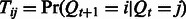, an emission probability matrix 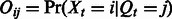and an m dimension prior distribution vector over the hidden states . With these model parameters, we can compute the joint distribution of the hidden and observed variables as and the distribution of the observed variables as .

We define the latent feature at position t of the sequence as the posterior distribution of the hidden variable Q_t, given the sequence up to position t:

(1)

This is also called the forward belief of the hidden variable Q_t, which captures the uncertainty about the ‘clean’ signal given the observed sequence up to position t (We can easily extend the approach to use the posterior distribution of Q_t given the entire sequence as features by involving both a forward and a backward recursion.) Note that is an m-dimensional vector that sums to 1. The latent features for the entire sequence according to the HMM are thus the concatenation of features at all positions, i.e. . Calculating requires us to marginalize over all previous hidden variables , which can be carried out in a recursive fashion:

(2)

Reexpressing the above relation in matrix form gives

(3)

where denotes the x_t-th row of the emission probability matrix . This matrix multiplication effectively implements the marginalization over variable .

Let and be a vector of all ones of size m. Equation (3) suggests a recursive algorithm that efficiently extracts the latent features.

(4)

which requires time, once we have learned the HMM parameters, i.e. the set of quantities . We note that we learn two HMMs and from training sequences, one for those with positive labels and the other for those with negative labels. Then for a new test sequence, we can extract two latent feature vectors, and , and use the concatenation of these two features as the sequence features.

One straightforward but computationally intensive way to learn the HMM is by using the EM. However, EM has the problem of slow convergence and convergence only to a local minimum. These two problems will affect the efficiency and efficacy of these latent feature extractions. To overcome the shortcomings of the EM algorithm, we use a fast and local-minimum-free spectral algorithm to learn an alternative parameterization of HMMs, which is described next.

3.2 Efficient spectral algorithm for latent features

Traditional HMM learning algorithms try to recover the parameters and . The resulting maximum-likelihood estimation problem is not convex and algorithms can only find a local optimum. These parameters and characterize the relations between hidden and observed variables that cannot be directly observed during training and are usually not uniquely identifiable. However, we may not need to recover them exactly to extract latent features. Instead, it is sufficient to recover them up to some invertible transformation if we subsequently learn a linear classifier such as a support vector machine. More specifically, suppose matrix of size is invertible. Define the transformed HMM parameters

(5)

Then we can compute the transformed latent feature as

(6)

since the invertible matrix cancels with during matrix multiplication. Then, the latent features of the final sequence that we use in our experiments are by concatenating the transformed features from positive and negative HMMs. It is easy to see that the transformed feature will achieve the same performance as the original one with a linear classifier because the transformation matrix can be incorporated into the classifier weight vector. That is, if we learn a binary classifier , then with will achieve the same classification accuracy.

A natural question is how to choose an such that the transformed parameters can be easier to estimate without using an EM algorithm. To solve this problem, we use a construction of by Hsu et al. (2012), which allows these transformed parameters to be estimated from just tri-gram information of the observed sequences. Formally, let be a triple of adjacent variables in the HMM and define the marginal probabilities of observation singletons, pairs and triples as

(7)

(8)

(9)

is an n dimensional vector, is an matrix and is a series of matrices indexed by x. Hsu et al. (2012) showed that setting directly links the above three quantities to the transformed parameters in (5), where is the leading m principal left singular vectors of . Specifically, the transformed parameters can be directly recovered from single sequence statics as

(10)

(11)

where computes the pseudo-inverse of a matrix.

Algorithm 1 Spectral learning of transformed HMM parameters.

Require: m—the number of hidden states, k—the number of nt to combine. Ensure: transformed HMM parameters .

• 1: Transform all training sequences by combining k consecutive nt into a ‘mega-observation’.

• 2: Use all triples from the transformed sequences to estimate and according to (12), (13) and (14).

• 3: Compute the Singular Value Composition (SVD) of , and let be the matrix of left singular vectors corresponding to the m largest singular values.

• 4: Compute transformed model parameters using (10) and (11).

The learning algorithm for HMMs is summarized in Algorithm 1. It first estimates the quantities in (7), (8) and (9) using training data

(12)

(13)

(14)

where D is the number of training sequences. These estimates are subsequently used to compute the transformed HMM model parameters according to (10) and (11). The algorithm has two parameters m and k that can be tuned by cross-validation. The major computation is an SVD of and hence the name ‘spectral algorithm’. We note that we learn two HMMs, one for the positive class and the other for the negative class. Then, we use both HMMs to extract features for each test sequence and concatenate the features, which are summarized in Algorithm 2.

Algorithm 2 Spectral latent feature extraction algorithm.

Require: —a test sequence, k—the number of nt to combine, and —learned HMM models for positive and negative classes. Ensure: spectral latent features .

• 1: Transform the input sequence by combining k adjacent nt into a ‘mega-observation’.

• 2: For , compute .

• 3: For , compute .

• 4: Concatenate features .

3.2.1 Fast implementation

The runtime of algorithm 1 is dominated by the SVD computation of an matrix , and the memory requirement is dominated by storing the tri-gram statistics for each x. One technical challenge is that n, the number of possible values of ‘mega-observation’, can grow as , exponential in k. It seems, at first sight, that we may need to decompose a huge matrix , and the memory requirement for is prohibitively large. However, most entries in these matrices are zero because some k-mers do not exist in the training sequences. Moreover, the total number of non-zero entries is at most the number of ‘mega-observations’ in the training set. Taking advantage of this property, we can do sparse matrix SVD and store all the tri-gram statistics in a sparse matrix, thus facilitating efficient computation and manipulation. The computational complexity thus grows linearly with the number of ‘mega-observations’ in the worst case.

3.3 Visualizing the importance of k-mers and positions

Besides accurately classifying the sequences, we are also interested in k-mers and positions that are most informative for motif classification. Sonnenburg et al. (2008) proposed positional oligomer importance matrices (POIMs) for WD kernels to analyze the importance of substrings in different locations of the sequence. Here, we also develop a technique for visualizing the importance of the k-mer at each position t for the classification problem based on our spectral latent features.

Intuitively, we want to use the contribution of the k-mer at position t to the support vector classifier as its importance score. In particular, we make use of the margin of a training sequence in the support vector machine. For example, if most positive sequences with large positive margins all contain k-mer AAGC at position t, then this k-mer is important for correct classifications. More formally, let the support vector classifier learned from our spectral latent features be and let the margin corresponding to a sequence be , where we use to indicate that the features are extracted from sequence . Then, we define the importance of k-mer at position t as

(15)

That is, given the sequences that have at position t, we compute the importance as the weighted sum of the margin of these sequences. In practice, we only have a finite number of training sequences, and we will use the finite sample average to estimate the importance score. That is, , where denotes the set of training sequences with k-mer occurring at position t.

Once we have computed the importance score for every k-mer at every position t, we can visualize it in a few different ways. One way is to visualize scores as a heatmap of k-mer versus sequence position. For longer k-mers, there are possible values that cannot be easily visualized. Instead, we sum the absolute values of all k-mer importance scores at each position, as is done in Sonnenburg et al. (2008), and visualize the importance score as a function of the position t. That is, .

4 RESULTS

4.1 Datasets

The proposed method was tested on the benchmark set proposed in Kalkatawi et al. (2012). The dataset contains 14 740 sequences (7370 with true poly(A) motifs—positive samples, and 7370 with false poly(A) motifs—negative samples) for the 12 main variants of human poly(A) motifs (see Table 1 for these variants and their respective sizes). For each variant, the number of positive sequences is equal to the number of negative sequences. Furthermore, for each variant, the positive motifs with the surrounding sequences were extracted from human mRNA and mapped back to the human genome, whereas the same numbers of negative motifs were randomly selected from human chromosome 21. Each sample is a candidate 6 nt poly(A) motif surrounded by 100 nt upstream and downstream. This represents a comprehensive benchmark set for poly(A) motifs in human DNA sequences. The goal is to predict which candidate motifs are true poly(A) motifs.

Table 1.

Comparison of the error rates of our method (HMM) with PPK, SPE and WD

Variants	Size	Error rate (%)					False-negative rate (%)					False-positive rate (%)
		PPK	SPE	WD	HMM	Rel	PPK	SPE	WD	HMM	Rel	PPK	SPE	WD	HMM	Rel
AATAAA	5190	—	23.08	23.72	18.59	19.45	—	21.93	23.70	18.54	15.47	—	24.24	23.74	18.65	23.05
ATTAAA	2400	27.13	20.17	18.29	16.21	19.63	32.50	22.83	21.50	18.17	20.44	21.75	17.50	15.08	14.25	18.57
AAGAAA	1250	31.28	14.72	16.72	9.36	36.41	37.12	14.08	19.68	11.36	19.32	25.44	15.36	13.76	7.36	52.08
AAAAAG	1230	15.04	13.25	7.80	5.45	58.90	25.20	8.94	8.46	6.02	32.73	4.88	17.56	7.15	4.88	72.22
AATACA	880	31.48	18.98	23.18	15.34	19.16	35.91	19.55	30.68	19.09	2.33	27.05	18.41	15.68	11.59	37.04
TATAAA	780	29.87	16.28	18.46	11.15	31.50	34.36	22.31	21.54	15.64	29.89	25.38	10.26	15.38	6.67	35.00
ACTAAA	690	40.72	24.35	30.29	16.96	30.36	43.48	28.41	39.42	20.00	29.59	37.97	20.29	21.16	13.91	31.43
AGTAAA	670	31.19	20.90	23.88	14.33	31.43	33.73	30.75	25.67	20.60	33.01	28.66	11.04	22.09	8.06	27.03
GATAAA	460	25.43	17.39	14.13	9.57	45.00	35.22	21.74	16.96	10.43	52.00	15.65	13.04	11.30	8.70	33.33
AATATA	410	29.51	15.85	18.78	9.27	41.54	31.22	23.90	25.85	14.63	38.78	27.80	7.80	11.71	3.90	50.00
CATAAA	410	32.68	18.78	22.20	12.68	32.47	40.98	22.93	27.80	20.49	10.64	24.39	14.63	16.59	4.88	66.67
AATAGA	370	24.05	8.11	14.86	5.14	36.67	22.16	6.49	9.73	6.49	0.00	25.95	9.73	20.00	3.78	61.11
Average	—	—	19.56	20.22	14.42	28.09	—	20.60	22.47	16.26	20.75	—	18.52	17.96	12.59	34.17

‘Average’ denotes the weighted average of the corresponding column. ‘Size’ denotes the number of samples for the corresponding motif variant. ‘Error rate’ is the proportion of false results in the dataset, which equals one minus accuracy. ‘False-negative rate’ is the proportion of true poly(A) motifs that are predicted to be false, which equals one minus sensitivity. ‘False-positive rate’ is the proportion of false poly(A) motifs that are predicted to be true, which equals one minus specificity. ‘Rel’ denotes the relative improvement of HMM with respect to SPE. The lowest error rate for each motif variant is indicated in bold. PPK could not finish running within 48 h on AATAAA.

4.2 Experimental settings

The proposed method was tested on each of the 12 datasets using 5-fold cross-validation. Each dataset was randomly partitioned into five subsets, four of which were used for training and validation, and the remaining one was used for testing in each fold.

We then searched for and using cross-validations (Supplementary Fig. S1). For each parameter combination and each dataset, two HMMs were learned for the positive samples and the negative ones in the training data. For each HMM, the parameters, , were learned by Algorithm 1. For each training sequence of 206 nt, the spectral latent feature vectors, , were then calculated for the positive and negative HMMs and concatenated (Algorithm 2). A linear Support Vector Machine (SVM) was then trained using these spectral latent features.

Given a testing sequence of 206 nt, the spectral latent feature vectors were extracted by Algorithm 2 using the learned HMMs for the same poly(A) motif. The concatenated feature vector was then given to the corresponding SVM model to predict whether it was a true poly(A) motif or a false one. The grid search for different parameters with respect to the training and testing errors indicated that the parameter ranges that had highest accuracy on the training set were and (Supplementary Fig. S1).

4.3 Comparison to other string kernels

We first compare the classification performance of the proposed method (HMM) with the previous state-of-the-art string kernels, namely, the PPK, SPE kernel and WD kernel. The best k for these alternative kernels, except PPK, was also searched using the cross-validation between three and seven, and we report here the best results. In Table 1, all reported errors are the average over the 5-fold cross-validation. It can be seen that the WD kernel compares favorably with the SPE kernel, with slightly higher false-negative rate and slightly lower false-positive rate. Our method, which simultaneously takes into account location information, sequence uncertainty and training labels, performs consistently and significantly better than PPK, SPE and WD. The PPK kernel has the worst results. As discussed in Section 2, PPK can suffer from severe overfitting by fitting each sequence to a separate HMM and it discards important discriminative information by not using the training labels.

Next, we compare the runtime of different methods using the largest two variants, AATAAA and ATTAAA. Our method is significantly faster than alternatives at training time, while being comparable in speed at test time (Table 2). In this experiment, the training time is equal to the time for kernel (or feature) computation for training data plus that for learning SVM models; and the test time is equal to the time for kernel (or feature) computation for test data plus that for classification. At training time, PPK, SPE and WD need to compute a square kernel matrix of size , and the associated SVM models need to be trained in the dual form. In contrast, our method computes a feature matrix of size , and the associated SVM model can be trained in the primal form (usually faster than in the dual form). At test time, PPK, SPE and WD need to compute the kernel values between each support vector (the number of support vectors can be large) and each test data point. In contrast, our method only computes a feature vector of length for each data point, and then performs an inner product with the learned SVM model , a vector of length .

Table 2.

Runtime comparisons on two variants AATAAA and ATTAAA for one train/test split, with k = 3 and all other parameters set to optimal

Time (s)	AATAAA				ATTAAA
	PPK	SPE	WD	HMM	PPK	SPE	WD	HMM
Training	—	46.16	37.38	7.59	2722.81	9.46	6.47	3.86
Testing	—	6.81	0.94	1.43	674.08	1.54	0.69	0.67

Note: PPK could not finish running within 48 h on AATAAA. The values in bold indicate better results.

4.4 Comparison to state-of-the-art method: the RF model

Table 3 compares the proposed method with a state-of-the-art by 5-fold cross-validation on the 12 variants of human poly(A) motifs: the RF model using domain-specific features by Kalkatawi et al. (2012). As shown in Table 3, our method is always significantly more accurate than RF (much lower error rates) and is more sensitive than RF on 11 out of the 12 variants. In fact, our method improves the error rates by 7–72% as compared with RF on the 12 motif variants. On average, our method has an improvement over RF in terms of the error rate, false-positive rate and false-negative rate by ∼26, 15 and 35%, respectively. These percentages imply that the significant improvement on the error rate is not just the result of a better trade off between sensitivity and specificity, but it is the result of being a better method in both senses. By comparing the results in Tables 1 and 3, it can be seen that the RF model outperforms other string kernels (PPK, SPE and WD) in terms of accuracy for poly(A) motif prediction. Our method that systematically extracts spectral latent features significantly improves upon RF and other string kernels on the same task. This supports our assumption that uncertainty and diversity information is important for this problem and there is a ‘clean’ DNA signal hidden in the observed sequences.

Table 3.

Comparison of our method (HMM) with RF

Variants	Size	Error rate (%)			False-negative rate (%)			False-positive rate (%)
		RF	HMM	Rel	RF	HMM	Rel	RF	HMM	Rel
AATAAA	5190	20.06	18.59	7.31	19.74	18.54	6.10	20.37	18.65	8.44
ATTAAA	2400	18.42	16.21	12.01	18.68	18.17	2.75	18.15	14.25	21.49
AAAAAG	1250	16.64	9.36	43.75	16.53	11.36	31.28	16.75	7.36	56.06
AAGAAA	1230	11.06	5.45	50.75	11.92	6.02	49.53	10.15	4.88	51.94
TATAAA	880	19.55	15.34	21.53	18.10	19.09	−5.47	20.87	11.59	44.46
AATACA	780	19.36	11.15	42.39	18.13	15.64	13.73	20.49	6.67	67.46
AGTAAA	690	27.83	16.96	39.07	25.24	20.00	20.76	29.92	13.91	53.50
ACTAAA	670	22.09	14.33	35.14	20.69	20.60	0.45	23.36	8.06	65.50
GATAAA	460	20.00	9.57	52.17	21.01	10.43	50.33	18.92	8.70	54.04
CATAAA	410	18.54	9.27	50.01	16.92	14.63	13.51	20.00	3.90	80.49
AATATA	410	24.88	12.68	49.02	24.12	20.49	15.06	25.59	4.88	80.94
AATAGA	370	18.38	5.14	72.06	19.37	6.49	66.51	17.32	3.78	78.15
Average	—	19.19	14.42	25.62	18.83	16.26	14.81	19.48	12.59	35.40

Note: The performance of both RF and HMM is evaluated on the same 5-fold cross-validation. ‘Rel’ denotes the relative improvement of HMM with respect to RF. The lowest value for each criterion of each motif variant is indicated in bold.

4.5 Visualizing importance scores of dimers and positions

Another advantage of our method over previous state-of-the-art poly(A) motif predictors is that our method can be used to visualize the importance of k-mers or positions to the prediction task. This can provide researchers or users a direct and intuitive way to study the patterns and characteristics of DNA sequences. More importantly, most previous studies on poly(A) motifs try to reveal statistics of the surrounding regions of true motifs. Our method, in contrast, can reveal patterns for false motifs at the same time.

In Figure 1, we present the importance scores for dimers (subsequences of 2 nt, e.g. AG) in determining whether or not a candidate poly(A) motif is a true motif. A number of interesting observations can be made about this figure:

Fig. 1.

Visualization of the importance of different dimers at different positions for the 12 variants of human poly(A) motifs. The x-axis gives the positions in the sequence. The y-axis lists all 16 possible dimers. The colors denote the levels of importance: the light green color for the positions 0–6 is the background color, which indicates that no effects differentiate true and false motifs; the darker the red, the more important the dimer at that position is to identifying true motifs; the darker the blue, the more important the dimer at that position is to identifying false motifs.

AA is an informative subsequence to differentiate true poly(A) motifs from false ones in all 12 variants of human poly(A) motifs. When AA appears frequently within 30 nt downstream of the candidate poly(A) motif, this strongly suggests that it is a true poly(A) motif. This is expected because the mRNA cleavage site is often 15–25 nt downstream of the poly(A) motif, and the region between the cleavage site and the motif is known to be A-rich (Retelska et al., 2006). Interestingly, when AA appears frequently within 100 nt upstream of the candidate motif, the candidate is likely to be a false motif.

CG is an interesting dimer. Its positions carry important information for determining both true and false poly(A) motifs. When CG appears beyond 40 nt upstream of the motif, this suggests that the motif is a true poly(A) motif. On the other hand, CG serves as a strong sign for false predictions in the immediate 20 nt downstream and then becomes a sign for true predictions for further downstream sequences. In Hu et al. (2005), it was found that −100/−41 and +41/+100 regions of poly(A) motifs are C- and G-rich regions. Our results suggest that looking at CG together rather than individually may capture more informative patterns.

TA or AT is one of the characteristics for false poly(A) motifs among all 12 variants. No matter if it appears frequently in downstream or upstream nt sequences of the candidate poly(A) motif, TA or AT suggests that the candidate is a false one. Between them, TA is more informative than AT to specify false motifs. On the one hand, our findings coincide with previous studies that TA and AT are important features around the poly(A) motifs and TA is more frequent than AT [e.g. the TATATA oligonucleotide is more over-represented than the ATATAT oligonucleotide (Hu et al., 2005; van Helden et al., 2000)]. On the other hand, our findings reveal that TA and AT appear much more often in sequences around the false motifs than around the true motifs. In van Helden et al. (2000); Hu et al. (2005), it was found that TATATA and ATATAT are the most over-represented oligonucleotides downstream of the poly(A) motifs. However, by analyzing the negative motifs, our results imply that although TA and AT appear often in positive motifs, they appear even more often in negative ones.

TG can determine false motifs at alternate positions upstream or downstream of the candidate motif of AATAGA (Fig. 1(l)). This is not the case for the two most frequent motifs, AATAAA and ATTAAA, which partially supports our hypothesis that the intrinsic characteristics of the frequent motifs and rare motifs are different. Thus, a good poly(A) motif predictor should have different models for different motif variants.

Figure 2 shows the importance scores for different positions with k from 1 to 5. Again, the 6 nt positions for the candidate motifs offer no information to the prediction. However, because the k-mers overlapping with the motif regions contain subsequences of the motifs, the motif regions do not have absolutely ‘zero’ importance. Again, we list key observations here:

Fig. 2.

Visualization of the importance of different positions for the 12 motif variants. The x-axis gives the position in the sequence. For each k from 1 to 5, the y-axis is the importance score of a position by summing over the absolute values of the importance for all possible k-mers at that position

The longer the subsequences are (bigger k), the smoother the importance curves are. This is expected because considering more nt at the same time will average the effects caused by individual positions.

In almost all the variants, the 50 nt downstream of the candidate motifs are informative. Specifically, motif variants AATAAA, CATAAA and AATATA have important information at the positions around the 25th nt downstream of the candidate motifs (Fig. 2a, j and k). This coincides with the fact that the mRNA cleavage site is 15–25 nt downstream of poly(A) motifs (van Helden et al., 2000; Retelska et al., 2006).

5 CONCLUSION AND FUTURE WORKS

In this article, we proposed a novel method to extract features from upstream and downstream regions of candidate poly(A) motifs in human DNA sequences. Our proposed spectral latent feature-based method achieves state-of-the-art results. The proposed method systematically explores the information encoded in nucleotide sequences by learning sequence dynamics and matching latent distributions on each position, and it can be easily extended to visualize the importance of subsequences and positions, thus providing a general method for sequence-based classification problems in bioinformatics. Our method can be directly applied to other sequence classification problems and achieve state-of-the-art results, such as the transcription start-site prediction and splice-site prediction (Supplementary Material S1 and Supplementary Table S1).

Our method, currently, requires a fixed length of upstream and downstream sequences for the training and testing data. Such prior knowledge has to be given as input. We are trying to generalize and extend our method to take varying lengths of sequences for different samples. Furthermore, there may be longer-range dependency between the latent variables, and HMMs of higher orders may be needed for the feature extraction purpose, for which junction tree-type algorithms can be applied (Parikh et al., 2012). Similar to the WD kernel with shifts (Rätsch et al., 2005), our method can also be straightforwardly extended to take shifted matches into account.

REFERENCES

- Ahmed F, et al. Prediction of polyadenylation signals in human DNA sequences using nucleotide frequencies. In Silico Biol. 2009;9:135–148. [PubMed] [Google Scholar]
- Akhtar MN, et al. Polyar, a new computer program for prediction of poly(a) sites in human sequences. BMC Genomics. 2010;11:646. doi: 10.1186/1471-2164-11-646. [DOI] [PMC free article] [PubMed] [Google Scholar]
- Beaudoing E, et al. Patterns of variant polyadenylation signal usage in human genes. Genome Res. 2000;10:1001–1010. doi: 10.1101/gr.10.7.1001. [DOI] [PMC free article] [PubMed] [Google Scholar]
- Bernstein P, Ross J. Poly(a), poly(a) binding protein and the regulation of mRNA stability. Trends Biochem. Sci. 1989;14:373–377. doi: 10.1016/0968-0004(89)90011-x. [DOI] [PubMed] [Google Scholar]
- Chang TH, et al. Characterization and prediction of mRNA polyadenylation sites in human genes. Med. Biol. Eng. Comput. 2011;49:463–472. doi: 10.1007/s11517-011-0732-4. [DOI] [PubMed] [Google Scholar]
- Cheng Y, et al. Prediction of mRNA polyadenylation sites by support vector machine. Bioinformatics. 2006;22:2320–2325. doi: 10.1093/bioinformatics/btl394. [DOI] [PubMed] [Google Scholar]
- Das AT, et al. A conserved hairpin motif in the r-u5 region of the human immunodeficiency virus type 1 RNA genome is essential for replication. J. Virol. 1997;71:2346–2356. doi: 10.1128/jvi.71.3.2346-2356.1997. [DOI] [PMC free article] [PubMed] [Google Scholar]
- Dempster AP, et al. Maximum likelihood from incomplete data via the EM algorithm. J. R. Stat. Soc. B. 1977;39:1–22. [Google Scholar]
- Graber JH, et al. In silico detection of control signals: mRNA 3′-end-processing sequences in diverse species. Proc. Natl Acad. Sci. USA. 1999;96:14055–14060. doi: 10.1073/pnas.96.24.14055. [DOI] [PMC free article] [PubMed] [Google Scholar]
- Hsu D, et al. A spectral algorithm for learning hidden Markov models. J. Comput. Syst. Sci. 2012;78:1460–1480. [Google Scholar]
- Hu J, et al. Bioinformatic identification of candidate cis-regulatory elements involved in human mrna polyadenylation. RNA. 2005;11:1485–1493. doi: 10.1261/rna.2107305. [DOI] [PMC free article] [PubMed] [Google Scholar]
- Jebara T, et al. Probability product kernels. J. Mach. Learn. Res. 2004;5:819–844. [Google Scholar]
- Ji G, et al. A classification-based prediction model of messenger rna polyadenylation sites. J. Theor. Biol. 2010;265:287–296. doi: 10.1016/j.jtbi.2010.05.015. [DOI] [PubMed] [Google Scholar]
- Kalkatawi M, et al. Dragon PolyA Spotter: predictor of poly(A) motifs within human genomic DNA sequences. Bioinformatics. 2013 doi: 10.1093/bioinformatics/btt161. [Epub ahead of print, doi: 10.1093/bioinformatics/btt161, April 15, 2013] [DOI] [PubMed] [Google Scholar]
- Kim KM, et al. Polya deletions in hereditary nonpolyposis colorectal cancer: mutations before a gatekeeper. Am. J. Pathol. 2002;160:1503–1506. doi: 10.1016/S0002-9440(10)62576-X. [DOI] [PMC free article] [PubMed] [Google Scholar]
- Langemeier J, et al. A complex immunodeficiency is based on u1 snrnp-mediated poly(a) site suppression. EMBO J. 2012;31:4035–4044. doi: 10.1038/emboj.2012.252. [DOI] [PMC free article] [PubMed] [Google Scholar]
- Legendre M, Gautheret D. Sequence determinants in human polyadenylation site selection. BMC Genomics. 2003;4:7. doi: 10.1186/1471-2164-4-7. [DOI] [PMC free article] [PubMed] [Google Scholar]
- Leslie C, et al. 2002. The spectrum kernel: A string kernel for svm protein classification. In Proceedings of the Pacific Symposium on Biocomputing, Vol. 7, pp 566–575. Hawaii, USA. [Google Scholar]
- Leslie C, et al. Mismatch string kernels for discriminative protein classification. Bioinformatics. 2004;20:467–476. doi: 10.1093/bioinformatics/btg431. [DOI] [PubMed] [Google Scholar]
- Leung AK, et al. Poly(adp-ribose) regulates stress responses and microrna activity in the cytoplasm. Mol. Cell. 2011;42:489–499. doi: 10.1016/j.molcel.2011.04.015. [DOI] [PMC free article] [PubMed] [Google Scholar]
- Liu H, et al. Dnafsminer: a web-based software toolbox to recognize two types of functional sites in dna sequences. Bioinformatics. 2005;21:671–673. doi: 10.1093/bioinformatics/bth437. [DOI] [PubMed] [Google Scholar]
- Lukashin A, Borodovsky M. Genemark.hmm: new solutions for gene finding. Nucleic Acids Res. 1998;26:1107–1115. doi: 10.1093/nar/26.4.1107. [DOI] [PMC free article] [PubMed] [Google Scholar]
- Parikh A, et al. Uncertainty in Artificial Intelligence. Catalina Island, USA: AUAI Press; 2012. A spectral algorithm for latent junction trees. [Google Scholar]
- Pastrello C, et al. Stability of bat26 in tumours of hereditary nonpolyposis colorectal cancer patients with msh2 intragenic deletion. Eur. J. Hum. Genet. 2006;14:63–68. doi: 10.1038/sj.ejhg.5201517. [DOI] [PubMed] [Google Scholar]
- Proudfoot NJ. Ending the message: poly(a) signals then and now. Genes Dev. 2011;25:1770–1782. doi: 10.1101/gad.17268411. [DOI] [PMC free article] [PubMed] [Google Scholar]
- Rätsch G, Sonnenburg S. Kernel Methods in Computational Biology. MIT press; 2004. Accurate splice site detection for caenorhabditis elegans; p. 277. [Google Scholar]
- Rätsch G, et al. Rase: recognition of alternatively spliced exons in c. elegans. Bioinformatics. 2005;21(Suppl. 1):i369–i377. doi: 10.1093/bioinformatics/bti1053. [DOI] [PubMed] [Google Scholar]
- Retelska D, et al. Similarities and differences of polyadenylation signals in human and fly. BMC Genomics. 2006;7:176. doi: 10.1186/1471-2164-7-176. [DOI] [PMC free article] [PubMed] [Google Scholar]
- Salamov AA, Solovyev VV. Recognition of 3′-processing sites of human mrna precursors. Comput. Appl. Biosci. 1997;13:23–28. doi: 10.1093/bioinformatics/13.1.23. [DOI] [PubMed] [Google Scholar]
- Sonnenburg S, et al. Arts: accurate recognition of transcription starts in human. Bioinformatics. 2006;22:e472–e480. doi: 10.1093/bioinformatics/btl250. [DOI] [PubMed] [Google Scholar]
- Sonnenburg S, et al. Accurate splice site prediction using support vector machines. BMC Bioinformatics. 2007;8(Suppl. 10):S7. doi: 10.1186/1471-2105-8-S10-S7. [DOI] [PMC free article] [PubMed] [Google Scholar]
- Sonnenburg S, et al. POIMs: positional oligomer importance matrices–understanding support vector machine-based signal detectors. Bioinformatics. 2008;24:i6–i14. doi: 10.1093/bioinformatics/btn170. [DOI] [PMC free article] [PubMed] [Google Scholar]
- Stanke M, Waack S. Gene prediction with a hidden Markov model and a new intron submodel. Bioinformatics. 2003;19(Suppl. 2):ii215–ii225. doi: 10.1093/bioinformatics/btg1080. [DOI] [PubMed] [Google Scholar]
- Tabaska JE, Zhang MQ. Detection of polyadenylation signals in human DNA sequences. Gene. 1999;231:77–86. doi: 10.1016/s0378-1119(99)00104-3. [DOI] [PubMed] [Google Scholar]
- van Helden J, et al. Statistical analysis of yeast genomic downstream sequences reveals putative polyadenylation signals. Nucleic Acids Res. 2000;28:1000–1010. doi: 10.1093/nar/28.4.1000. [DOI] [PMC free article] [PubMed] [Google Scholar]
Associated Data
This section collects any data citations, data availability statements, or supplementary materials included in this article.