Influence of a priori Information, Designs, and Undetectable Data on Individual Parameters Estimation and Prediction of Hepatitis C Treatment Outcome

Abstract

Hepatitis C viral kinetic analysis based on nonlinear mixed effect models can be used to individualize treatment. For that purpose, it is necessary to obtain precise estimation of individual parameters. Here, we evaluated by simulation the influence on Bayesian individual parameter estimation and outcome prediction of a priori information on population parameters, viral load sampling designs, and methods for handling data below detection limit (BDL). We found that a precise estimation of both individual parameters and treatment outcome could be obtained using as few as six measurements in the first month of therapy. This result remained valid even when incorrect a priori information on population parameters was set as long as the parameters were identifiable and BDL data were properly handled. However, setting wrong values for a priori population parameters could lead to severe estimation/prediction errors if BDL data were ignored and not properly accounted in the likelihood function.

Chronic infection with hepatitis C virus (HCV) is a liver disease that affects about 150 million people worldwide and is directly responsible of about 350,000 deaths every year.¹ The goal of anti-HCV treatment is to achieve a sustained virologic response (SVR), defined as undetectable serum HCV RNA 24 weeks after treatment cessation.² HCV is classified into six major genotypes (GT) with HCV GT-2/3 being the second cause of chronic hepatitis C (after GT-1), accounting for ~15–20% of infection in Western countries.³

Since 2001, the combination of pegylated interferon (peg-IFN) and ribavirin (RBV) is the backbone of anti-HCV treatment with SVR rate of ~50 and 80% in patients infected with GT-1 and GT-2/3, respectively.^4,5,6 In 2011, the approval of two protease inhibitors marked a new era of HCV therapy with a dramatic improvement in SVR rates in patients infected with HCV GT-1.^{7,8,9,10,11,12,13} However, there is no clear evidence that PIs are beneficial in GT-2/3 patients.^14,15,16,17 Even though new treatment, such as nucleotide analogs may be effective against GT-2/3,¹⁸ their cost and the fact that peg-IFN/RBV is already efficient makes bitherapy likely to remain essential in the treatment against HCV GT-2/3.^15,17 Because peg-IFN/RBV therapy is associated with several significant side effects and high costs,¹⁹ several efforts have been made to evaluate the possibility of treatment individualization.²⁰

For that purpose, one can use viral kinetic models whose parameters have a high predictive value of treatment outcome.^21,22 However, the use of these models is limited by the fact that frequent viral load data in the first weeks following treatment initiation are required to obtain precise estimation of the parameters. One way to improve the precision of individual parameter is to consider that the population parameters are known a priori and to perform Bayesian estimation of individual parameters. Thus, this method combines a priori information of population parameters gathered from previous studies and individual viral load data prospectively obtained in a patient. This approach is similar to what is done in therapeutic drug monitoring using population pharmacokinetic models.^23,24

However, the relevance of this approach is still contingent on the study design.²⁵ In practice, the difficulty to frequently assess viral load levels often gives predictions based on a limited number of viral load data within each patient. We would therefore like to evaluate the quality of individual parameter estimation and treatment outcome prediction using a realistic design based on a small number of short-term observations.

A common challenge in analyzing HCV kinetic data is the fact that a large proportion of viral load data are below the detection limit (BDL). Several studies have shown that naive approaches that omit or impute BDL data at an arbitrary value led to biased population parameter estimates, and this can be corrected by taking BDL data into account in the likelihood function.^26,27,28,29 However, these studies focused on the population parameters and did not evaluate whether and how these methods improved Bayesian individual parameter estimation.

Here, our goal is to evaluate, by simulation and in the context of HCV GT-2/3, the influence of a priori population model, of viral load sampling designs and of methods for handling BDL data when estimating individual parameters and treatment response.

Results

Description of the simulated data

The percentages of BDL data were equal to 57.4, 27.8, 37.7, and 38.5 with designs D_24w, D_4w, D_{4w_sparse}, and D_{4w_challenge}, respectively (see “Methods”). The SVR rate was equal to 78.4%, consistent with the rate of 80% reported in the literature for HCV GT-2/3.^5,6 Of note, 53.6% of the simulated patients had already eradicated the virus by week 12 (W12) of treatment. Non-SVR patients were classified as relapsers (undetectable HCV RNA at the end of treatment becomes detectable 24 weeks later), null-responders (HCV RNA declines from baseline <1 log₁₀ at all time), or rebounders (HCV RNA declines from baseline >1 log₁₀ then rebounds under treatment), accounting for 7.6, 2.3, and 11.7% of our simulated population, respectively. Furthermore, two types of rebounders were considered: patients having a breakthrough (rebounds after a period being undetectable) or a partial virologic response (rebounds after a declining period but never being undetectable), accounting for 3.3 and 8.4% of the simulated population, respectively.

Individual parameter estimation

Table 1 gives the mean relative bias (MRE), relative root mean square error (RRMSE), and shrinkage of the parameters β, δ, c, and ε obtained for each design using true (M_true) or false population models (M_δε, M_β) and methods that omit (OMIT) or handle BDL data in the likelihood function (LBA).

Table 1. Mean relative bias, RRMSE, and shrinkage (in %) of β, δ, c, ε for different scenarios^a.

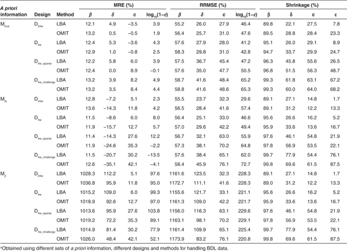
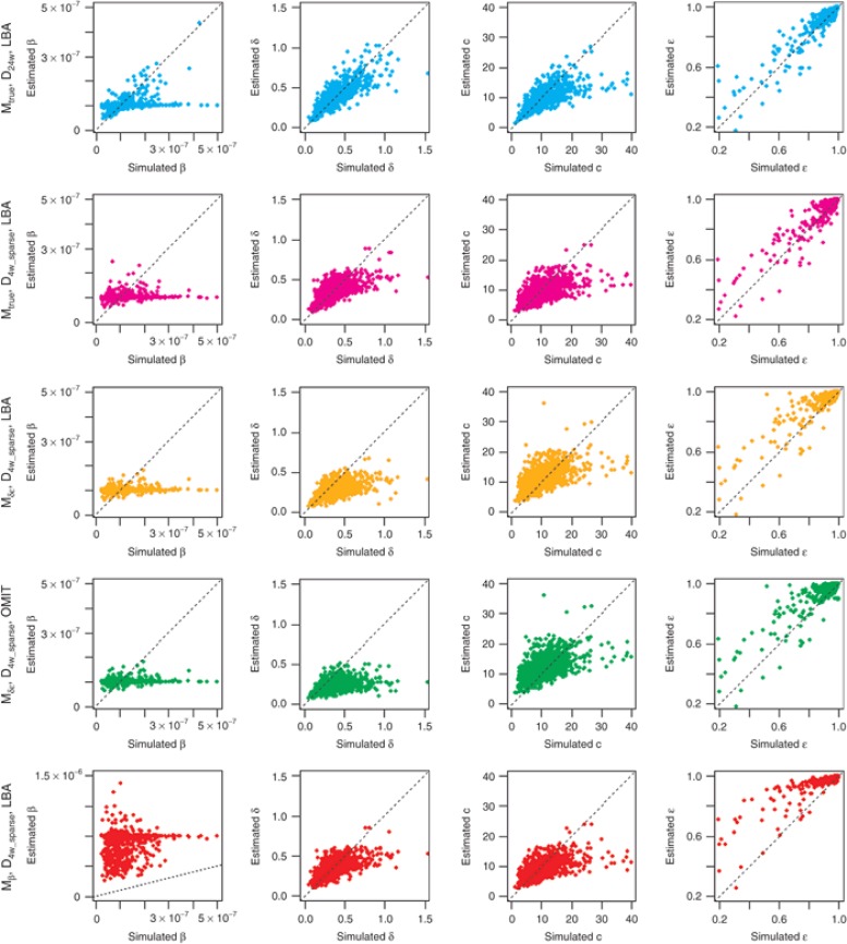
Even when the a priori information on population parameters was correct (i.e., M_true), individual parameters were estimated with some bias and with the most informative design (D_24w), RRMSE for the infectivity rate β was still equal to 55.4%. Moreover, β consistently had an extremely high shrinkage, >80% regardless of designs (Table 1 and Figure 1). This is due to the fact that this parameter can be precisely estimated only if there is a virologic rebound, a feature that was observed in only 11.7% of patients. The three other parameters c, δ, and ε could be estimated with a shrinkage and a RRMSE <50% as long as viral load data in the first week of treatment were available. As expected, the precision of parameter estimation deteriorates with less frequent sampling designs and the RRMSE for δ, c, and log₁₀(1-ε), increased by ~30, 60, and 15%, respectively, when using the D_{4w_sparse} as opposed to the D_4w design. Similarly, the shrinkage for δ, c, and ε increased by ~80, 90, and 300%, respectively, when using the D_{4w_sparse} as opposed to the D_4w design. Surprisingly, a correct handling of BDL data did not critically improve the estimation of individual parameters when true a priori population parameters were set: for all parameters, only a small difference was found between LBA and OMIT methods using MRE (<6%) and RRMSE (<4%) as evaluation criteria, regardless of designs.

Figure 1.

Scatter plots of estimated values vs. simulated values for β, δ, c, ε under five selected cases (top to bottom): M_true_D_24w_LBA, M_true_D_{4w_sparse}_LBA, M_δε_D_{4w_sparse}_LBA, M_δε _D_{4w_sparse}_OMIT, and M_β _D_{4w_sparse}_LBA. The dotted line is the identity line. Lower left corner graph has a different scale on the y-axis compared to the other plots as in this scenario, β was fixed at a value that was 10 times higher than the true value to estimate individual parameters.

Setting the fixed effect of δ and ε at false values (M_δε) naturally led to larger estimation errors, especially for δ and c. Since in this model the a priori value for δ was less than half of the true value (0.14 vs. 0.32 day⁻¹, respectively), the individual values for this parameter were consistently underestimated with an increasing relative bias, compared with that obtained with true information: for instance, using the design D_{4w_challenge}, relative bias going from 3.9% with true a priori population parameters up to 20.7% with false a priori information even when correctly handling BDL data. As the rate of the first phase of viral decline is proportional to c × ε (see “Methods”), the estimates of these two parameters were correlated. This explains why setting a lower ε than the one used to generate the data (90% instead of 99.6%) led to an overestimation of c. This was particularly visible when considering designs without frequent samplings where c is poorly identifiable. For instance, the relative bias increased from 6% to 28% and RRMSE increased from 45% to 63% when comparing the D_{4w_sparse} design under the true and false model. However, the quality of parameter estimates remained reasonable (RRMSE < 50%) when using designs with frequent sampling in the first week, at least as long as BDL data were correctly handled. Indeed, and unlike what was seen when using the true population parameters, omission of BDL data dramatically deteriorated parameter precision. This was particularly noticeable for δ where MRE doubled when omitting instead of correctly handling BDL data: for instance, using D_4w design, MRE increased from −8.6% with LBA method to −15.7% when BDL data were omitted.

However, the result that setting false population parameters is not critical to achieve precise parameter estimates (at least as long as BDL data are correctly handled) becomes wrong if parameters are poorly identifiable. Indeed, extremely high errors were obtained for all parameters when setting β to a value 10-fold larger than the true one (M_β, Table 1).

Prediction of treatment outcome

We then investigated the impact of individual parameter estimation on treatment outcome prediction for the simulated patients. Results are presented in Figure 2. The influence of simulated individual parameters on treatment outcome was assessed in Supplementary Material 1 online.

Figure 2.

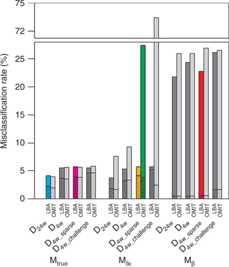
Misclassification rates (sum of false-positive (filled with pattern) and false-negative rates) of prediction of treatment outcome for a 24-week treatment in different scenario.

In case of correct a priori information, the prediction of individual treatment outcome was very good: even with the most challenging design where individual parameter estimates were biased, the misclassification rate was lower than 6%. The choice of designs did not have much impact on the prediction of treatment outcome although a slightly better prediction was obtained with rich design. With less information (by shortening or reducing sampling frequency), more false-positive (FP) responses were obtained as the prediction tended to be influenced by the response of the profile using the mean parameter values, i.e., SVR with this parameter regime (Supplementary Material 2 online) Of note, the relevance of this approach can be examined by comparing misclassification rate using viral kinetic model with what would be obtained if no information was available. In that case, one would predict SVR in all patients, leading to an error rate of 21.6%, in which all are FP.

In case of false a priori information about δ and ε, we found, as previously, that a correct handling of BDL data was necessary to obtain good prediction and omitting BDL data dramatically increased false-negative (FN) responses (Supplementary Material 2 online), especially when designs become less informative: for instance, in comparison with a correct handling of BDL data, FN increased from 1.6% to 23.5% and 0.5% to 71.5% when omitting BDL data in designs D_{4w_sparse} and D_{4w_challenge}.

If one would predict SVR using rapid virologic response (RVR), defined as undetectable HCV RNA at W4 after treatment initiation, the misclassification rate would be still very good (6.9%). This, actually, means that the use of a viral kinetic model and data in the first month improved treatment outcome prediction by only 1.4% and 1.2% if a priori information was true or not, respectively. Thus the use of viral kinetic models does not bring, with this parameter regime, a critical benefit. This may be due to the fact that we evaluated the ability of treatment outcome prediction in a very favorable case where treatment outcome was highly correlated with the virologic response at W4. This is why we also compared the predictive ability of RVR and modeling in the case of shorter treatment duration of 12 weeks. In this more challenging case, the superiority of modeling approach was clear, with misclassification rates of only 14.6% and 19.2% when using correct or false a priori information, respectively, as compared with 50% when using RVR (Supplementary Material 3 online).

Whereas using M_δε did not much deteriorate the prediction quality, assuming false a priori information on β led to very high error rates (>20%) for all designs, even when BDL data were correctly handled, which is the consequence of a poor estimation of all individual parameters (see Supplementary Material 1 online).

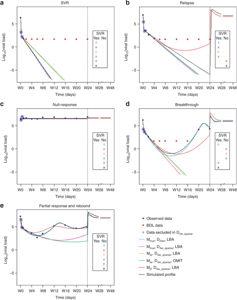
We illustrated the influence of different factors on individual estimation and outcome prediction using examples of five typical patterns of virologic responses found in the simulated population (Figure 3). As expected, long design allowed obtaining individual fits close to the true, i.e., simulated profiles, especially when a virologic rebound occurred. With lower δ and ε, it is not surprising that M_δε predicted higher treatment duration to achieve SVR, compared to the true model. This explained high rate of FN obtained with this false information (Supplementary Material 2 online). Similarly, a larger number of treatment failures were predicted with higher β, which is associated with more chances of virologic rebound.

Figure 3.

Examples of some individual fits for the different patterns of virologic responses obtained with different models, designs and BDL data handling methods:(a) SVR, (b) relapse, (c) null-response, (d) breakthrough, (e) partial response and rebound. The solid lines represent the predicted trajectories with the designs M_true_D_24w_LBA (blue), M_true_D_{4w_sparse}_LBA (magenta), M_δε_D_{4w_sparse}_LBA (orange), M_δε_D_{4w_sparse}_OMIT (green), and M_β_D_{4w_sparse}_LBA (red) and the true profile (black). Vertical line indicates the end of treatment (24 weeks). Observed and BDL data are presented as blue and red diamonds, respectively. Data that were not included in sparse designs are circled. 4-week designs do not contain measurements after W4. Simulation is stopped when the cure boundary is achieved, indicating that the patient has SVR.

Discussion

Here we evaluated the role of a priori information, designs, and methods for handling BDL data in the prediction of individual virologic response and thus the ability of using viral kinetic models to individualize therapy in HCV GT-2/3 infected patients. Unlike what is usually done, we focused on individual parameters and assumed that the population parameters (i.e., the mean and the between-patient variability) were known to estimate individual parameters using Bayesian approach.

Using true a priori population parameters, precise estimation of individual parameters and good prediction of treatment outcome were obtained. Obviously, a major limitation of Bayesian approaches is that a priori values of the population parameters are required. This a priori information could be wrong, for instance if coming from a set of patients with different characteristics. This is why we also evaluated the robustness of this approach when the population parameters were different from the “true” parameters, i.e., those used for data simulation. Our results showed that setting wrong population parameters did not dramatically deteriorate individual parameters estimation as long as the parameters were identifiable (such as δ and ε). Importantly, satisfactory parameter estimation was obtained using a clinically relevant design with a limited number of data points (<6) and a last data point at W4. Therefore, the estimation of viral kinetic parameters with this approach could allow for a rapid prediction of treatment outcome. In the case of β, a parameter that can be correctly estimated at individual level only in patients who have a virologic rebound (11.7% of our simulated population), assuming a higher value led to very large estimation errors in all individual parameters. The combination of these largely biased parameters led to high prediction errors for treatment response (see Supplementary Material 1 online).

BDL data is another factor that could lead to substantial bias. Interestingly, ignoring BDL data did not lead to significant bias as long as a priori population parameters were true. However, a correct handling of undetectable data became critical when population parameters were wrong, and we showed that this can be achieved by likelihood-based approaches that rigorously calculate the information contained in BDL data.

Here we predicted the treatment outcome in a patient using the individual parameter estimates, which are the modes of a posteriori distribution, and therefore defining a yes/no response. In order to apply this approach to clinical practice, one would need to evaluate uncertainty of treatment outcome prediction by using the whole a posteriori distribution of individual parameters, i.e., by incorporating uncertainty on individual parameter estimates. This could be done by reconstructing the a posteriori distribution, for instance using MCMC methods.

The ultimate goal of viral kinetic modeling is to allow for individual parameter estimation and treatment tailoring. To achieve this goal, pharmacometricians will need reliable models and appropriate sampling designs that can provide precise parameter estimation. The information contained in a design can be a priori evaluated and optimized using the Fisher information matrix. This approach became a standard tool for pharmacokinetic/pharmacodynamic studies using NLMEM and was implemented in several software such as PFIM, PopED, POPDES, and POPT.³⁰ However, viral kinetic models have specific features that are not always properly addressed in these software such as the large proportion of BDL data^31,32 and the need to achieve a good level of precision of both population and individual parameters.^33,34 Clearly, optimal design at population and individual levels may differ, and theoretical studies are needed to provide relevant designs at both levels.

Here we studied the ability of modeling approach in the prediction of IFN-based treatment outcome in HCV GT2/3 patients using a standard viral kinetic model. More sophisticated models are now being developed to explain complex viral kinetic patterns observed with new direct acting antiviral agents.³⁵ Further studies will be necessary to suggest relevant designs to precisely estimate treatment outcome with this new generation of treatments and models.

Methods

Viral kinetic model. In this study, we used a standard HCV model with liver regeneration^36,37 given by the following set of equations:

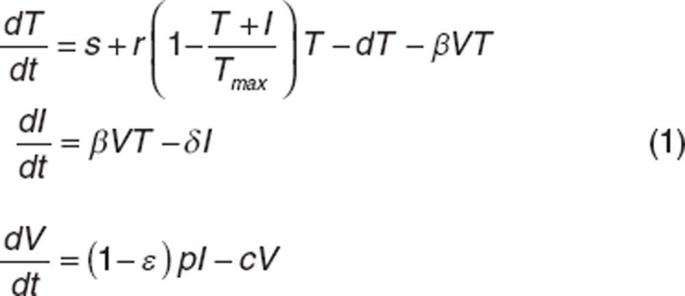The model considers target cells T, infected cells I, and free virus V. Targets cells are produced at rate s, proliferate with rate r, die at rate d and become infected at rate β. Infected hepatocytes die at rate δ and release virions at rate p per cell. Virions are cleared from serum with rate c. Peg-IFN acts by blocking virion production, p, with effectiveness ε varying between 0 and 1. We assumed that the viral infection system before treatment initiation (t = 0) is at steady state. If only viral load data are measured, the parameters s, r, d, T_max, p cannot be identified individually and therefore were usually set to values found in literature in parameter estimation.^22,25,38 In this study, we investigated only four identifiable parameters β, δ, c and ε, which are also the most clinical relevant parameters. Indeed, in most patients treated with peg-IFN, viral load initially declines in a biphasic manner. This biphasic decline is captured by c, δ and ε. The first phase has a rate c × ε and leads to a viral load decline equal to log₁₀(1−ε), which reflects drug effectiveness. Subsequently, viral load declines with a slower but persistent rate approximately equal to δ × ε. If ε is high enough, viral load will continuously decrease during treatment. Otherwise, a virologic rebound may occur,³⁷ and the kinetics of viral rebound will depend on the value of β: higher values of β give earlier rebounds.

Statistical model. Let i denote the ith individual (i = 1,…,N) and j the jth measurement of an individual (j = 1,…, n_i where n_i is the number of observations for individual i). The statistical model for the viral load y_ij measured in individual i at time t_ij is given by:

where f : nonlinear viral kinetic model, identical for all individuals,

θ_i: individual parameters vector,

e_ij: residual error supposed to follow normal distribution N(0,^σ2).

Because viral kinetics is simulated on long time period, it can happen that viral load takes values very close to 0. In that case, numerical errors may give a negative value for the viral load. This is why, unlike what is usually done, we evaluated the viral load in its natural scale and not in the log₁₀ scale.

The individual parameters θ_i can be decomposed into fixed effects µ = {β, δ, c, ε} representing mean effects of the population and random effects η_i specific for each individual. It is assumed that η_i ~ N(0, Ω) with Ω defined as the variance–covariance matrix in which, each diagonal elements ω_q representing the variance of the qth component of the random effect vector _ηi. We assumed log-distribution for β, δ, c (qth parameter):

and logit-distribution for ε:

The population parameters vector ψ is composed of {µ, Ω, σ }

Bayesian individual parameter estimation. In NLMEM, individual parameters are estimated using Bayesian approach. They are calculated as the Maximum a posteriori (MAP), i.e., the mode of the posterior distribution. Let ψ be the known population parameters vector and let be the conditional distribution of _ηi. The MAP estimate of _ηi is given by

As µ is known, once is estimated, can be easily calculated.

In presence of data below limit of detection (LOD), the distribution is calculated by:

where is the probability density function, and is the cumulative density function of normal distribution with mean m, variance v, evaluated at x.

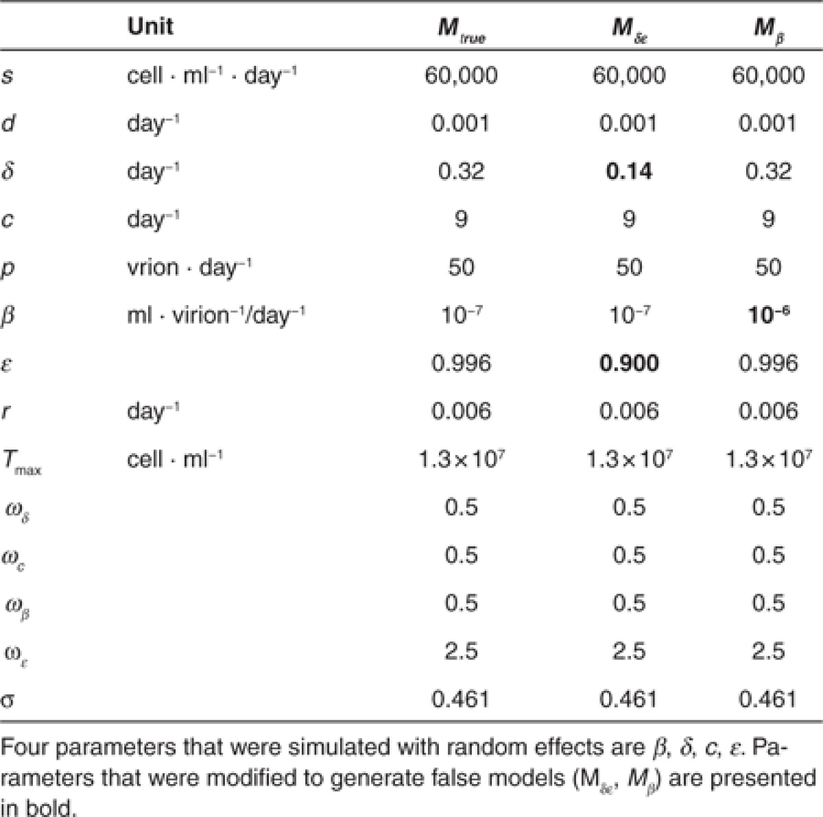
Simulation study. This simulation study aimed at mimicking the viral response observed in HCV GT-2/3 infected patients during peg-IFN/RBV. The values for ε, δ, and c in GT-2/3 infected patients are based on literature.³⁹ For β, this parameter has never been estimated in this population, and therefore we use a value being in the range of possible values and close to those estimated in HCV GT-1 infected patients.^36,40 We used population parameters presented in the M_true column (Table 2) for data simulation.

Table 2. Parameter values of the different viral kinetic models in response to treatment (M_true, M_δε, M_β).

Four nested designs D_{4w_challenge} ⊂ D_{4w_sparse} ⊂ D_4w ⊂ D_24w were considered. The richest design, D_24w, contains 12 sampling times until the end of the treatment (days 0, 1, 4, 7, W2, 4, 6, 8, 12, 16, 20, 24). D_4w (days 0, 1, 4, 7, W2, 4) does not have any data after W4, D_{4w_sparse} (days 0, 7, W2, 4) does not have any data after W4 and during the first week and D_{4w_challenge} has only one measurement at baseline and W4 (day 0, W4).

We simulated N = 1,000 vectors of random effects _ηi to calculate individual parameters θ_i from the population parameters of the true model. We then predicted the viral kinetics in these 1,000 in silico patients using the mathematical model (Eq.1). Residual errors were then simulated and added to viral load data for all sampling times of D_24w to obtain dataset for D_24w design. As the four designs are nested, to generate datasets for other designs, we selected the simulated viral loads corresponding to the sampling times of the design of interest (Supplementary Material 4 online). As the same data of the same 1,000 simulated individuals were used to generate all the datasets, all the differences obtained in results were not due to Monte Carlo errors.

We considered a limit of detection LOD = 45 IU/ml. Since successful therapy leads to SVR, i.e., the eradication of HCV, we hypothesized the existence of a threshold, called “cure boundary,” under which infection is considered eradicated. Following what has been done previously, we assumed that this threshold corresponds to having <1 infected cell in the whole extracellular body fluid, assumed to be 15 L.²² Although this cure boundary has not yet proven biologically correct, prediction of treatment outcome using this threshold has been shown to match SVR rate observed during peg-IFN based therapy.²² If the course of infected cells crossed the cure boundary, we considered that SVR was achieved and no viral relapse could occur afterwards. All viral loads obtained after achieving the cure boundary are considered undetectable.

To evaluate the impact of a priori information on individual parameter estimation and outcome prediction, we modified fixed effects of some parameters to generate two false models (Table 2): for M_δε, we set δ and ε to the values obtained in GT-1 infected patients; for M_β we set β to the upper limit of possible values found in literature.⁴⁰

To estimate individual parameters for 1,000 simulated patients, individual random effects η_i were first estimated and then used to calculate individual parameters. We supposed that population parameters were already known and fixed them at different sets of a priori values corresponding to M_true, M_δε, M_β to perform MAP. BDL data were handled using two approaches: taking into account BDL data in the likelihood function (likelihood-based approach or LBA) or omitting all BDL observations in the dataset (OMIT).

To evaluate the ability of estimation of the component q of an individual parameter, we used the following criteria: Mean Relative Error (MRE) and Relative Root Mean Square Error (RRMSE) defined by:t

For ε, we evaluate the MRE and RRMSE of log₁₀(1−ε).

We also used shrinkage (Shr) to evaluate the quality of individual parameter estimates (Eq. 9). A low shrinkage (<50%) indicates that individual parameter is correctly estimated.

Once estimated, individual parameters were then used to simulate the individual predicted profiles of target cells, infected cells, and viral loads assuming a 24- or 12-week treatment. If infected cells were predicted to achieve the cure boundary during treatment, the predicted treatment outcome is having SVR and vice versa.

By comparing the predicted treatment outcome with the true (simulated) response, we calculated the percentage of false-negative FN (patients having SVR predicted to remain infected), false-positive FP (uncured patients predicted to have SVR) and of misclassification MC (sum of FN and FP). Using these criteria, we compared the quality of treatment outcome prediction between different scenarios and with the case where no individual observation is available. To evaluate the gain of using modeling approach compared to empirical rules used in clinics, we also evaluated the predictive ability for SVR of “rapid virologic response,” RVR—defined as undetectable viral load at W4. We also considered a shorter treatment that was stopped at W12 in order to evaluate the ability of outcome prediction in a challenging case.

All simulation was done using R 2.14.0. Parameter estimation (Supplementary Material 5 online) was performed using MONOLIX 4.1.2.

Conflict of Interest

T.H.T.N. has a research grant from Novartis. J.Y. and M.L. are working for Novartis, in Modeling and Simulation department. As an associate editor for CPT: PSP, F.M. was not involved in the review or decision process for this paper.

Study Highlights

References

- World Health Organization Hepatitis C. Fact sheet No. 164., < ., < http://www.who.int/mediacentre/factsheets/fs164/en/index.html >( Revised July 2012 [Google Scholar]
- Maylin S., et al. Eradication of hepatitis C virus in patients successfully treated for chronic hepatitis C. Gastroenterology. 2008;135:821–829. doi: 10.1053/j.gastro.2008.05.044. [DOI] [PubMed] [Google Scholar]
- Mangia A., Mottola L., Piazzolla V. Update on the treatment of patients with non-genotype 1 hepatitis C virus infection. Clin. Infect. Dis. 2013;56:1294–1300. doi: 10.1093/cid/cis1195. [DOI] [PubMed] [Google Scholar]
- Manns M.P., et al. Peginterferon alfa-2b plus ribavirin compared with interferon alfa-2b plus ribavirin for initial treatment of chronic hepatitis C: a randomised trial. Lancet. 2001;358:958–965. doi: 10.1016/s0140-6736(01)06102-5. [DOI] [PubMed] [Google Scholar]
- Zeuzem S., et al. Peginterferon alfa-2b plus ribavirin for treatment of chronic hepatitis C in previously untreated patients infected with HCV genotypes 2 or 3. J. Hepatol. 2004;40:993–999. doi: 10.1016/j.jhep.2004.02.007. [DOI] [PubMed] [Google Scholar]
- von Wagner M., et al. Peginterferon-alpha-2a (40KD) and ribavirin for 16 or 24 weeks in patients with genotype 2 or 3 chronic hepatitis C. Gastroenterology. 2005;129:522–527. doi: 10.1016/j.gastro.2005.05.008. [DOI] [PubMed] [Google Scholar]
- Bacon B.R., HCV RESPOND-2 Investigators et al. Boceprevir for previously treated chronic HCV genotype 1 infection. N. Engl. J. Med. 2011;364:1207–1217. doi: 10.1056/NEJMoa1009482. [DOI] [PMC free article] [PubMed] [Google Scholar]
- Flamm S.L., et al. Boceprevir with peginterferon alfa-2a-ribavirin is effective for previously treated chronic hepatitis C genotype 1 infection. Clin. Gastroenterol. Hepatol. 2013;11:81–87.e4; quiz e5. doi: 10.1016/j.cgh.2012.10.006. [DOI] [PubMed] [Google Scholar]
- Kwo P.Y., SPRINT-1 investigators et al. Efficacy of boceprevir, an NS3 protease inhibitor, in combination with peginterferon alfa-2b and ribavirin in treatment-naive patients with genotype 1 hepatitis C infection (SPRINT-1): an open-label, randomised, multicentre phase 2 trial. Lancet. 2010;376:705–716. doi: 10.1016/S0140-6736(10)60934-8. [DOI] [PubMed] [Google Scholar]
- McHutchison J.G., PROVE1 Study Team et al. Telaprevir with peginterferon and ribavirin for chronic HCV genotype 1 infection. N. Engl. J. Med. 2009;360:1827–1838. doi: 10.1056/NEJMoa0806104. [DOI] [PubMed] [Google Scholar]
- McHutchison J.G., PROVE3 Study Team et al. Telaprevir for previously treated chronic HCV infection. N. Engl. J. Med. 2010;362:1292–1303. doi: 10.1056/NEJMoa0908014. [DOI] [PubMed] [Google Scholar]
- Poordad F., SPRINT-2 Investigators et al. Boceprevir for untreated chronic HCV genotype 1 infection. N. Engl. J. Med. 2011;364:1195–1206. doi: 10.1056/NEJMoa1010494. [DOI] [PMC free article] [PubMed] [Google Scholar]
- Zeuzem S., REALIZE Study Team et al. Telaprevir for retreatment of HCV infection. N. Engl. J. Med. 2011;364:2417–2428. doi: 10.1056/NEJMoa1013086. [DOI] [PubMed] [Google Scholar]
- Lenz O., et al. Virologic response and characterisation of HCV genotype 2-6 in patients receiving TMC435 monotherapy (study TMC435-C202). J. Hepatol. 2013;58:445–451. doi: 10.1016/j.jhep.2012.10.028. [DOI] [PubMed] [Google Scholar]
- Mangia A., Mottola L. Treatment of non-genotype 1 hepatitis C virus patients. Curr. Gastroenterol. Rep. 2012;14:87–93. doi: 10.1007/s11894-011-0235-3. [DOI] [PubMed] [Google Scholar]
- Reiser M., et al. Antiviral efficacy of NS3-serine protease inhibitor BILN-2061 in patients with chronic genotype 2 and 3 hepatitis C. Hepatology. 2005;41:832–835. doi: 10.1002/hep.20612. [DOI] [PubMed] [Google Scholar]
- Wartelle-Bladou C., Le Folgoc G., Bourlière M., Lecomte L. Hepatitis C therapy in non-genotype 1 patients: the near future. J. Viral Hepat. 2012;19:525–536. doi: 10.1111/j.1365-2893.2012.01634.x. [DOI] [PubMed] [Google Scholar]
- Gane E.J., et al. Nucleotide polymerase inhibitor sofosbuvir plus ribavirin for hepatitis C. N. Engl. J. Med. 2013;368:34–44. doi: 10.1056/NEJMoa1208953. [DOI] [PubMed] [Google Scholar]
- Fried M.W. Side effects of therapy of hepatitis C and their management. Hepatology. 2002;36:S237–S244. doi: 10.1053/jhep.2002.36810. [DOI] [PubMed] [Google Scholar]
- Mihm U., Herrmann E., Sarrazin C., Zeuzem S. Review article: predicting response in hepatitis C virus therapy. Aliment. Pharmacol. Ther. 2006;23:1043–1054. doi: 10.1111/j.1365-2036.2006.02863.x. [DOI] [PubMed] [Google Scholar]
- Arends J.E., et al. Plasma HCV-RNA decline in the first 48 h identifies hepatitis C virus mono-infected but not HCV/HIV-coinfected patients with an undetectable HCV viral load at week 4 of peginterferon-alfa-2a/ribavirin therapy. J. Viral Hepat. 2009;16:867–875. doi: 10.1111/j.1365-2893.2009.01143.x. [DOI] [PubMed] [Google Scholar]
- Snoeck E., et al. A comprehensive hepatitis C viral kinetic model explaining cure. Clin. Pharmacol. Ther. 2010;87:706–713. doi: 10.1038/clpt.2010.35. [DOI] [PubMed] [Google Scholar]
- Williams P.J., Ette E.I. The role of population pharmacokinetics in drug development in light of the Food and Drug Administration's ‘Guidance for Industry: population pharmacokinetics'. Clin. Pharmacokinet. 2000;39:385–395. doi: 10.2165/00003088-200039060-00001. [DOI] [PubMed] [Google Scholar]
- Rousseau A., Marquet P. Application of pharmacokinetic modelling to the routine therapeutic drug monitoring of anticancer drugs. Fundam. Clin. Pharmacol. 2002;16:253–262. doi: 10.1046/j.1472-8206.2002.00086.x. [DOI] [PubMed] [Google Scholar]
- Guedj J., Bazzoli C., Neumann A.U., Mentré F. Design evaluation and optimization for models of hepatitis C viral dynamics. Stat. Med. 2011;30:1045–1056. doi: 10.1002/sim.4191. [DOI] [PubMed] [Google Scholar]
- Bergstrand M., Karlsson M.O. Handling data below the limit of quantification in mixed effect models. AAPS J. 2009;11:371–380. doi: 10.1208/s12248-009-9112-5. [DOI] [PMC free article] [PubMed] [Google Scholar]
- Samson A., Lavielle M., Mentré F. Extension of the SAEM algorithm to left-censored data in nonlinear mixed-effects model: application to HIV dynamics model. Comput. Stat. Data. An. 2006;51:1562–1574. [Google Scholar]
- Thiébaut R., et al. Estimation of dynamical model parameters taking into account undetectable marker values. BMC Med. Res. Methodol. 2006;6:38. doi: 10.1186/1471-2288-6-38. [DOI] [PMC free article] [PubMed] [Google Scholar]
- Yang S., Roger J. Evaluations of Bayesian and maximum likelihood methods in PK models with below-quantification-limit data. Pharm. Stat. 2010;9:313–330. doi: 10.1002/pst.400. [DOI] [PubMed] [Google Scholar]
- Mentré F, et al. Current use and developments needed for optimal design in pharmacometrics: a study performed amongst DDMoRe's EFPIA members. CPT Pharmacometrics Syst. Pharmacol. 2013;2:e46. doi: 10.1038/psp.2013.19. [DOI] [PMC free article] [PubMed] [Google Scholar]
- Dumont C., Mentré F., Gaynor C., Brendel K., Gesson C., Chenel M. Optimal sampling times for a drug and its metabolite using SIMCYP(®) simulations as prior information. Clin. Pharmacokinet. 2013;52:43–57. doi: 10.1007/s40262-012-0022-9. [DOI] [PubMed] [Google Scholar]
- Vong C., Ueckert S., Nyberg J, Hooker A.C.Handling below limit of quantification data in optimal trial designAnnual Meeting of the Population Approach Group in Europe. 2012Abstract 2578; < http://www.page-meeting.org/?abstract=2578 >. [Google Scholar]
- Combes F., Retout S., Frey N., Mentré F.Prediction of shrinkage of individual parameters using the Bayesian information matrix in non-linear mixed effect models with evaluation in pharmacokinetics Pharm. Resdoi:10.1007/s11095-013-1079-3. [DOI] [PubMed]
- Merlé Y., Mentré F. Bayesian design criteria: computation, comparison, and application to a pharmacokinetic and a pharmacodynamic model. J. Pharmacokinet. Biopharm. 1995;23:101–125. doi: 10.1007/BF02353788. [DOI] [PubMed] [Google Scholar]
- Chatterjee A., Guedj J., Perelson A.S. Mathematical modelling of HCV infection: what can it teach us in the era of direct-acting antiviral agents. Antivir. Ther. (Lond.) 2012;17:1171–1182. doi: 10.3851/IMP2428. [DOI] [PMC free article] [PubMed] [Google Scholar]
- Dahari H., Ribeiro R.M., Perelson A.S. Triphasic decline of hepatitis C virus RNA during antiviral therapy. Hepatology. 2007;46:16–21. doi: 10.1002/hep.21657. [DOI] [PubMed] [Google Scholar]
- Dahari H., Lo A., Ribeiro R.M., Perelson A.S. Modeling hepatitis C virus dynamics: liver regeneration and critical drug efficacy. J. Theor. Biol. 2007;247:371–381. doi: 10.1016/j.jtbi.2007.03.006. [DOI] [PMC free article] [PubMed] [Google Scholar]
- Wu H., Zhu H., Miao H., Perelson A.S. Parameter identifiability and estimation of HIV/AIDS dynamic models. Bull. Math. Biol. 2008;70:785–799. doi: 10.1007/s11538-007-9279-9. [DOI] [PubMed] [Google Scholar]
- Bochud P.Y., et al. IL28B polymorphisms predict reduction of HCV RNA from the first day of therapy in chronic hepatitis C. J. Hepatol. 2011;55:980–988. doi: 10.1016/j.jhep.2011.01.050. [DOI] [PubMed] [Google Scholar]
- Dahari H., Shudo E., Cotler S.J., Layden T.J., Perelson A.S. Modelling hepatitis C virus kinetics: the relationship between the infected cell loss rate and the final slope of viral decay. Antivir. Ther. (Lond.) 2009;14:459–464. [PMC free article] [PubMed] [Google Scholar]
Associated Data
This section collects any data citations, data availability statements, or supplementary materials included in this article.