

Abstract
Summary: Non-linear calibration is a widely used method for quantifying biomarkers wherein concentration-response curves estimated using samples of known concentrations are used to predict the biomarker concentrations in the samples of interest. The R package nCal fills an important gap in the open source, stand-alone software for performing non-linear calibration. For curve fitting, nCal provides a new implementation of a robust, Bayesian hierarchical five-parameter logistic model. nCal supports a simple graphical user interface that can be used by laboratory scientists, and contains functionality for importing data from the multiplex bead array assay instrumentation.
Availability: The R package ‘nCal’ is available from http://cran.r-project.org/web/packages/nCal/ under GPL-2 or later.
Contact: yfong@fhcrc.org
Supplementary information: Supplementary information is available in the form of an R package vignette at the above repository and an FAQ at http://research.fhcrc.org/youyifong/en/resources/ncal.html.
1 INTRODUCTION
Non-linear calibration is a widely used method for quantifying biomarkers in biomedical studies. There are two stages in non-linear calibration. In the first stage, a concentration-response curve is estimated for each assay run using observed outcome for standard samples with known concentrations. An assay run refers to a batch of samples run closely in time and space, e.g. all samples run on a single microplate. In the second stage, point estimates and confidence bounds are estimated for the biomarker concentrations in the samples of interest.
Many laboratories use commercial software for performing non-linear calibration. These include general purpose programs like GraphPad Prism and StatLIA, as well as assay-specific programs like MasterPlex and Bio-Plex Manager for the multiplex bead array assay, which is becoming a common assay for quantifying protein concentrations. Besides being expensive and hard to automate, these programs provide relatively simple single-curve fitting methods. Furthermore, they often lack proper precision estimates for the estimated concentrations.
The R package nCal provides two sets of curve-fitting methods. The first, implemented through another R package drc (Ritz and Streibig, 2005), is an estimating equation-based method that is equivalent to those available from most existing non-linear calibration software. The second, implemented within nCal, is a robust Bayesian random effects model-based approach (Fong et al., 2012). It allows borrowing of information across multiple assay runs for the same biomarker, incorporates prior information regarding the curve-to-curve variability and provides flexible models for the experimental noise. After obtaining a curve fit via either approach, nCal estimates the biomarker concentrations in the samples of interest and computes variance estimates for the estimated concentrations.
nCal does not have as extensive a graphical user interface as its commercial counterparts do, but it does contain a simple graphical user interface based on the R package gWidgets that allows non-R users to perform non-linear calibration. nCal also provides a function that imports data from the Excel files of Luminex® results that have been output by a Bio-Plex instrument’s software.
2 METHODS
Sigmoid-shaped concentration-response curves can be approximated well by five-parameter logistic (5PL) curves. Let Yik denote the experimental outcome, where i indexes assay runs and k indexes standard samples. Let  denote the 5PL function with parameter
  . Estimating equation-based methods solve the following optimization problem for each assay run:
where g is a penalty function. For least square method,  ; for robust method,
  can be
  , a trim function or a winsorization function (Ritz and Streibig, 2005). The estimated concentration for a sample with observation y is then
  .
.
A Bayesian random effects 5PL model was considered by Fong et al. (2012) and Davidian and Giltinan (1995) and can be described as follows.
 is assumed to have a multivariate normal distribution with mean
  and precision Ω. The experimental noise
  can be modeled as having a normal distribution; for robust methods, it can be modeled as having a Student’s t-distribution, a mixture of two normal distributions or a latent first-order autoregressive process (Fong et al., 2012). We assume weakly informative priors on
  and the parameters of the noise distribution, and substantive priors on Ω (Fong et al., 2012). The hyperparameters are listed in the Supplementary Information. Posterior samples are drawn using Just Another Gibbs Sampler (JAGS) (Plummer, 2003). We take the median of the posterior samples of
  to be its point estimate, and the median of the posterior samples of
  to be the estimated concentration for a sample with observation y.
As in Davidian and Giltinan (1995), the variance of the estimated concentration can be decomposed into two components. The first component assumes that the concentration-response curve is perfectly known and the variability comes from the variability of y. It can be estimated as  for both sets of curve fitting methods, where
  is the estimated variance of the experimental noise. The second component assumes that y is perfectly measured and the variability comes from the variability of the curve estimate. For the estimating equation-based methods, it can be estimated by
  , where
  is the estimated variance–covariance matrix of
  . For the Bayesian random effects model-based methods, it can be estimated by the variance of the posterior samples of
  .
.
3 EXAMPLE SESSIONS
We illustrate the use of nCal through two examples (see Supplementary Information for the complete R code and more detailed explanation of the output). In the first example, we simulate a dataset with one assay run and four samples of interest. To perform non-linear calibration, we call
> res=ncal(log(fi) ∼expected_conc, dat, bcrm.fit=TRUE)
The Boolean argument bcrm.fit controls whether to use bcrm, which implements the Bayesian random effects model, or drm from the drc package, which implements the estimating equation methods for curve fitting. res is a data frame, each row of which corresponds to one sample of interest. ncal also creates a plot with four panels (Supplementary Information nCal vignette Supplementary Fig. S1 and S2), showing the curve fit, the estimated concentrations for the samples of interest and the precision profiles. From the two figures, we see that both curve fitting methods lead to similar calibration results for this example.
In the second example, we analyze a dataset containing four assay runs, one of which is affected by multiple outliers.
> fit.bcrm=bcrm(log(fi) ∼expected_conc, dat, error.model=”gh_t4”, informative.prior=T) > for (i in 1:4) { fit.drm=drm(log(fi) ∼expected_conc, data= dat, subset=assay_id==paste(”Run”,i), fct=LL.5(),robust=”median”) plot(fit.drm, type=”all”, main=p) plot(get.single.fit(fit.bcrm, paste(”Run”, i)),add=T) }
Figure 1 shows that the two methods produce similar results for Runs 1, 3 and 4, but differs significantly for Run 2. Figure 1 also shows the curve fits by Prism with the robust option. By borrowing information across assay runs, bcrm appears more successful at reducing the influence of multiple outlying observations than drm and Prism.
Fig. 1.
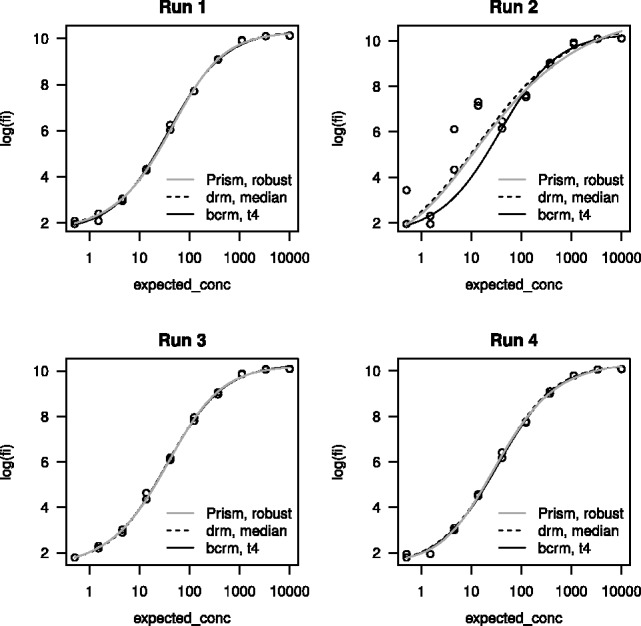
Example II. Robust curve fits from Prism, drm and bcrm
ACKNOWLEDGEMENTS
The authors thank members of the Lab Data Operations at SCHARP for assay data quality control. They also thank the members of the CRAN team for testing and distributing the package. The authors are grateful to the editor, the associate editor and the referees for their constructive comments.
Funding: This work was supported by the National Institute of Allergy and Infectious Diseases (NIAID) [UM1-AI-068618] to the HIV Vaccine Trials Network, the Bill and Melinda Gates Foundation [OPP1032317] to the Collaboration for AIDS Vaccine Discovery and the NIAID [AI104370-01] to Y.F.
Conflict of interest: none declared.
REFERENCES
- Davidian M, Giltinan D. Nonlinear models for repeated measurement data. Vol. 62. USA: Chapman & Hall/CRC, Boca Raton, FL; 1995. [Google Scholar]
- Fong Y, et al. A robust Bayesian random effects model for nonlinear calibration problems. Biometrics. 2012;68:1103–1112. doi: 10.1111/j.1541-0420.2012.01762.x. [DOI] [PMC free article] [PubMed] [Google Scholar]
- Plummer M. Proceedings of the 3rd International Workshop on Distributed Statistical Computing. 2003. JAGS: a program for analysis of Bayesian graphical models using Gibbs sampling. 2003, p. 20–22. Vienna, Austria. [Google Scholar]
- Ritz C, Streibig J. Bioassay analysis using R. J. Stat. Software. 2005;12:1–22. [Google Scholar]