

Significance
Social ties are more common between individuals with similar traits, a feature known as homophily. Ties are also known to be stronger between individuals with multiple common acquaintances. Both of these two properties constrain the flow of information and ideas in social networks. We study time-dependent communication patterns in a large mobile phone communication dataset and show that both of these two properties are in fact stronger than can be observed in any static snapshot of a communication network. The methods developed to obtain these results can be used more generally to study various time-dependent networks.
Keywords: social networks, human dynamics
Abstract
Recent studies on electronic communication records have shown that human communication has complex temporal structure. We study how communication patterns that involve multiple individuals are affected by attributes such as sex and age. To this end, we represent the communication records as a colored temporal network where node color is used to represent individuals’ attributes, and identify patterns known as temporal motifs. We then construct a null model for the occurrence of temporal motifs that takes into account the interaction frequencies and connectivity between nodes of different colors. This null model allows us to detect significant patterns in call sequences that cannot be observed in a static network that uses interaction frequencies as link weights. We find sex-related differences in communication patterns in a large dataset of mobile phone records and show the existence of temporal homophily, the tendency of similar individuals to participate in communication patterns beyond what would be expected on the basis of their average interaction frequencies. We also show that temporal patterns differ between dense and sparse neighborhoods in the network. Because also this result is independent of interaction frequencies, it can be seen as an extension of Granovetter’s hypothesis to temporal networks.
Social networks have been studied since the early 20th century, and their significance to the performance and well-being of individuals is now widely recognized (1, 2). The availability of electronic communication records—data on mobile phone calls, e-mails, tweets, and messages in social networking sites—has, however, created unprecedented opportunities for studying social networks (3, 4), allowing the analyzing of human interaction networks at the societal scale (5–7), studying their mesoscale structure (8), and carrying out experiments with tens of millions of subjects (9).
Communication records are typically studied by constructing an “aggregate network” where the nodes correspond to people, edges denote their relations as inferred from the communication data, and tie strengths are accounted for by edge weights representing communication frequency. Although this approach has been immensely successful, it disregards all information contained in the detailed timings of communication events. As an example, individuals who appear highly connected in the aggregate network might only interact with a small number of acquaintances at a time (10).
Human communication has been shown to have rich temporal structure (11–13), and one of the challenges of computational social science is to understand this rich behavior. Although temporal inhomogeneities can be partially attributed to circadian and weekly patterns (12, 14), detailed analysis has shown that they have more fundamental origins (13, 15–17). Human communication is known to be intrinsically bursty (11, 13, 18, 19) and contain strong pairwise correlations of interaction times (13).
“Homophily” refers to the well-documented tendency of individuals to interact with others similar to them with respect to various social and demographic factors (20–22). Because social networks act as conduits of information, homophily limits the information that individuals can receive. Although sex homophily is known to be less strong than homophily by age, race, or education (22), sex-related differences in communication have been documented at least in instant messaging (23), Facebook (24), and the use of both domestic (25) and mobile phones (26). However, not much is known about patterns involving multiple individuals, or the influence of factors such as sex or age on communication patterns. This is the focus of the present article.
Increased awareness about the importance of temporal information in various empirical datasets has led to the emergence of the concept of “temporal networks,” a general framework for studying time-dependent interactions between nodes (27). Here, we study communication patterns of multiple individuals within this framework. We represent communication records as a “colored” temporal network where node colors are used to refer to individuals’ attributes. We then identify “temporal motifs” in these data to summarize their mesoscale temporal structure (28) and develop a null model that identifies differences between the relative occurrence of node colors in temporal motifs so that these differences are independent of the structure of the aggregate network. This choice of null model assures that all results presented in this article are independent of any previous results obtained by studying static communication networks where link weights correspond to communication frequency.
Using a large dataset of mobile phone calls, we find significant differences in the occurrence of mesoscale communication patterns. We identify “temporal homophily,” overrepresentation of temporal patterns that contain similar nodes beyond that predicted by the structure of the aggregate network. By using event colors in addition to node colors, we also find consistent and robust differences between events occurring in dense and sparse neighborhoods of the aggregate network. Because this result is independent of the aggregate network, it can be seen as a temporal extension of Granovetter’s hypothesis about the correlation of local density and edge weights (29).
Temporal Motifs in Colored Networks
Temporal motifs are analogous to “network motifs” introduced by Milo and coworkers in 2002 (30, 31) as classes of isomorphic subgraphs more common in the empirical network than in some “null model.” Because the use of a null model to define motifs has proven problematic (32) (see also the discussion in SI Text), we adopt the practice of Onnela et al. (33) and use the term “motif” more generally to denote a class of equivalent subgraphs, independent of their statistical significance in comparison with some reference.
As defined by Kovanen et al. (28), temporal motifs are equivalence classes of valid temporal subgraphs. To understand what this means, consider a temporal network 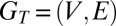 where the events E represent interactions between the nodes V: An event
 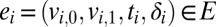 from node
  to
to  starts at time
  and has duration
  . (We only consider directed events, but the changes needed to handle undirected events are negligible.) In this article, we also presume that the temporal network is colored: There is a mapping
  from nodes to the set of possible colors C. Colors can be used to distinguish different node types.
Given a time window  , two events are “
 -adjacent” if they share at least one node and the time difference between them is no longer than
  . With adjacency, we can define connectivity: Two events are “
 -connected” if there exists a sequence of
  -adjacent events between them. A connected “temporal subgraph” can now be defined as a set of events where any two events are
  -connected. If the events in this set are also consecutive for each node, the temporal subgraph is “valid.” [This constraint is needed to restrain motif counts. Consider an out-star with n events that all take place within
  . This out-star contains
  temporal subgraphs with k events, but only
  valid temporal subgraphs. The same problem is also encountered with static motifs, but in that case no equally natural solution is available (34).]
Finally, a temporal motif m is an equivalence class of valid temporal subgraphs when two subgraphs are considered equivalent if their underlying colored graphs are isomorphic and their events occur in the same order (Fig. 1B). Given a temporal network, “motif count”  is the number of valid temporal subgraphs in equivalence class m. Algorithms described in ref. 28 allow calculating
  for small motifs in colored temporal networks with up to 109 events. In the rest of this article, we will use the term “motif” to refer to colored temporal motifs.
Fig. 1.
(A) A schematic presentation of two temporal networks. The upper one has clear temporal structure, whereas the lower one is random; however, both give rise to the same aggregate network. (B) Two examples on identifying temporal motifs. Starting from a temporal network (Left), we first identify temporal subgraphs (Center), and then the temporal motif corresponding to each subgraph (Right). Note that temporal motifs do not contain information about the identities of nodes or the exact times of events, but do retain information about node colors and the temporal order of events. (C) The six possible uncolored two-event temporal motifs whose colored variants are used in our analysis.
Null Model for Differences Between Node Types
Unfortunately, just knowing motif counts is not very informative: With nothing to compare with, it is impossible to say whether a given count is high or low. The approach suggested by Milo et al.—and the de facto standard in motif analysis—is to compare motif counts to those in a null model, a suitably randomized version of the empirical data. It is, however, far from obvious what exactly can be learned from such comparison (see ref. 32 and SI Text). We argue that the key to using null models is to craft the difference between the empirical data and the null model so that it is explicitly known and matches the research question at hand. It is this difference that gives an interpretation for the deviation between  and
and  .
.
Thus, to quantify the effect of node types, we construct a null model where the reference count  can be interpreted as the weighted average of untyped motif counts, with weighting done by the structure of the aggregate network (Materials and Methods). This null model tests the null hypothesis that motif counts do not depend on node types, given the structure of the weighted aggregate network. Conditioning on the aggregate network is crucial, as it means that any difference observed between
  and
and  cannot be explained by differences in the number of nodes of each type, variations in the activity of node types, or preferred connectivity patterns. In other words, the results are purely temporal: They are independent of anything observable in the aggregate network.
Evaluating Deviation from the Null Model.
To tell whether the null hypothesis is true—that there are no differences between node types given the aggregate network—we calculate the z scores as follows:
 |
where  and
and  are the mean and SD of the count in the null model. If the null hypothesis is true, z scores are expected to have zero mean and unit variance.
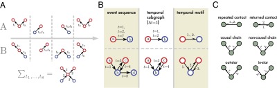
One should be cautious in making conclusions based on z scores beyond falsifying the null hypothesis. As z scores depend on data size, it is not uncommon to find motifs with  in large datasets; this only means that the null hypothesis is even more unlikely to be true. Neither should one conclude that motifs with
  are “explained” by the null model—the null model was just proven to be false, so it cannot explain our observations (SI Text).
However, because we can interpret the deviation between the null model and the empirical data, we can use the null model to measure effect size. We do this by calculating the ratio  . (The ratio score is an unstandardized measure of effect size. Such measures are generally considered to be the best practice in reporting results; see, e.g., ref. 35.) Because
  is the motif count under the null hypothesis that node types have no effect,
  reveals how much more or less common a motif is because of node types.
Synthetic Data.
To illustrate what this null model can reveal, we first apply it to synthetic data where we know exactly what there is to find. These synthetic data have two types of nodes, red and blue, with events occurring in such a fashion that those causal chains are more common where the first event takes place between nodes of the same color (see Materials and Methods for details). This pattern, however, is only visible in the event data; the weighted aggregate network shows no difference between red and blue nodes.
Fig. 2 shows the z-score distribution for all two-event motifs in these synthetics data. As expected, the null hypothesis is false: There are two peaks at  corresponding to the causal two chains. The motifs with
  are those where the first two nodes have the same color, and these motifs have
  : They are 18% more common than expected if there were no difference between node types.
Fig. 2.

The null model correctly identifies temporal differences in synthetic data. The figure shows the distribution of z scores for all two-event motifs, averaged over 50 datasets. For most motifs  because there are no differences between node colors. The peak at
  corresponds to the four causal chains where the first event occurs between nodes of the same color. Because expected motif count is defined by the average count of uncolored motifs, the peak at
  contains the four remaining causal chains where the first event occurs between nodes of different color.
Results
We now turn to study a mobile phone dataset that contains 600 million calls during a period of 6 mo between 6.3 million anonymized customers (Materials and Methods). As the data include information on the time and duration of calls, it can be represented as a temporal network. Node types are formed by combining the sex, age group, and payment type (prepaid or postpaid mobile subscription plan; Materials and Methods) of customers.
Our analysis focuses on two-event motifs for simplicity (Fig. 1C). Larger motifs are not only more demanding computationally but also more laborious to analyze: There are already 56,448 different two-event motifs with the 24 node types created by combining sex, age group, and payment type. All results have been calculated with  min, which allows reasonable time for intentional reactions but should not include too many serendipitously simultaneous events. The results are not, however, particularly sensitive to the value of
  (see SI Text for details).
Node Types Affect Motif Counts.
We first check whether the null hypothesis is true or false—whether node types affect motifs counts beyond what can be expected based on the aggregate network—by plotting the distribution of z scores (Fig. 3A). The distribution does not have zero mean or unit variance; instead, about 35% of motifs have  . The null hypothesis is clearly false, and we can conclude that motif counts are not independent of node types.
Fig. 3.

The empirical data contain temporal differences between node types that are destroyed by randomizing the data. The plots show the distribution of z scores for all two-event motifs with  in (A) the first month of empirical data, (B) the same data after shuffling node types, and (C) after shuffling event times. The gray curve shows a Gaussian distribution with zero mean and unit variance for reference.
For comparison, Fig. 3B shows the same distribution after shuffling node types, and Fig. 3C after shuffling event types (Materials and Methods). In both cases, the distributions suggest that the null hypothesis is true. Indeed, after randomizing node types there can be no differences between them even though the data still contain the same “untyped” temporal subgraphs as the original data. The time-shuffled data, on the other hand, have exactly the same aggregate network as the original data. However, because event times are now uncorrelated, all differences between node types are explained by the structure of the aggregate network.
There Is Temporal Homophily.
There is temporal homophily in interaction patterns beyond the homophily observed in the aggregate network.
Fig. 3A shows that there are differences between node types; we will now look at what these differences are. We first investigate whether homophily also manifests at the level of contact sequences, i.e., whether there is temporal homophily, a tendency of similar individuals to jointly participate in interaction patterns beyond the homophily observed in the aggregate network.
To this end, we calculate the average  of two-event motifs where all nodes have the same age group, sex, or payment type, or agree for all of these attributes. This average is then compared with the average
  of all other motifs. The results are presented in Table 1. Note that the values shown in this table are averages over a large number of motifs; as we will soon show, individual motifs often exhibit significantly larger variations. For motifs involving only two individuals, the only statistically significant difference is an underexpression of the returned-call motif for participants of the same payment type. This is due to frequent patterns where a prepaid customer calls a postpaid customer, who then immediately calls back, as illustrated in Fig. 4A.
Table 1.
Temporal motifs reveal the existence of temporal homophily
| Motif | A | G | P | A ∧ G ∧ P |
| Repeated call | 1.08, 1.11 | 1.12, 1.09 | 1.09, 1.13 | 1.09, 1.11 |
| Returned call | 1.04, 1.01 | 1.02, 1.01 | 0.98, 1.06 | 1.02, 1.02 |
| Noncausal chain | 1.05, 1.03 | 1.05, 1.03 | 1.05, 1.01 | 1.18, 1.03 |
| Causal chain | 1.03, 1.02 | 1.04, 1.02 | 1.05, 0.98 | 1.16, 1.02 |
| Out-star | 1.12, 1.03 | 1.06, 1.03 | 1.07, 1.01 | 1.32, 1.04 |
| In-star | 1.09, 1.04 | 1.07, 1.04 | 1.03, 1.06 | 1.16, 1.04 |
The columns correspond to motifs where all participants are similar with respect to different attributes: age (A), sex (G), payment type (P), or all three (A ∧ G ∧ P). The first value in each cell is the mean  for motifs where all nodes have the same attribute value (for example, all have the same age in column A). The second value gives the mean for all other motifs. If the first value is larger than the second, the motif has homophily with respect to that attribute: Motifs where all nodes have the same value are relatively more common than others. Welch’s t test was used to test for equality; bold denotes
  and italic denotes
  (with Bonferroni correction for 42 hypotheses, including those only shown in SI Text).
Fig. 4.

The most common temporal motifs exhibit shared properties. (A) The four most common returned-call motifs. The numbers inside the nodes denote the age group (18–26, 27–32, 33–38, 39–45, 46–55, or 56–80; the value shown is the weighted average rounded to closest integer). The open nodes denote postpaid and filled prepaid customers; red denotes female, and blue, male. The arrows denote events, and the numbers next to them show their temporal order. In all four cases, the first call takes place from the prepaid (filled node) to the postpaid (open node) customer. The number below each motif shows the relative occurrence compared with the null model. (B) The four most common out-star motifs. In all four cases, the two receivers have the same age, a pattern that is typical for the most common out-stars.
More complex motifs—chains and stars—exhibit more evidence of temporal homophily. Motifs where the participants agree with respect to all three attributes are significantly more common, and star-like motifs are overrepresented also when the participants agree with respect to only one attribute. As illustrated in Fig. 4B, out-stars also exhibit an interesting pattern where the ages of the two recipients are correlated. The strongest effect is typically observed for similarity of payment type; note, however, that payment type is likely to correlate with various other socioeconomic factors. Results for text messages are qualitatively similar (SI Text).
Chains and Stars are Overexpressed for Females.
To analyze sex differences in temporal motifs, we calculate the average  separately for motifs where all participants are either male or female. The results are presented in Table 2. No difference is observed for repeated and returned calls, but for all other motifs the all-female case is overexpressed, and all-male case slightly underexpressed.
Table 2.
All-female star and chain motifs are more common than respective all-male motifs
| Motif | Female | Male |
| Repeated calls | 1.11, 1.11 | 1.13, 1.10 |
| Returned calls | 1.02, 1.01 | 1.02, 1.02 |
| Noncausal chain | 1.08, 1.02 | 1.01, 1.04 |
| Causal chain | 1.08, 1.01 | 0.98, 1.03 |
| Out-star | 1.10, 1.03 | 1.01, 1.04 |
| In-star | 1.11, 1.03 | 1.01, 1.05 |


Local Edge Density Correlates with Temporal Motifs.
The algorithm used for identifying temporal motifs also allows distinguishing between different event types (28). Here, we use event types to study the correlation between local network density and temporal patterns. This is closely related to Granovetter’s hypothesis (29) that states that in social networks there is a positive correlation between edge weights and local network density, where the latter can be measured for example by the number of triangles around an edge. Granovetter’s hypothesis has already been verified in mobile phone call data (5). Because our analysis factors out the entire structure of the weighted aggregate network, the results presented here are independent of this classic hypothesis.
We use clique percolation (36) to create a dichotomy for local edge density: Event  is a “dense event” if the edge
  of the aggregate network is inside a four-clique community, and otherwise
  is a “sparse event.” We find clear and robust differences in temporal behavior between dense and sparse edges, as summarized in Table 3. Single-edge motifs—repeated and returned calls—are more common on sparse edges, whereas all other two-event motifs follow an opposite pattern and are relatively more common in dense parts of the network. One possible explanation is that sparse parts of the network offer less opportunities for motifs that occur on two edges. Were this the case, one would expect motifs with one dense and one sparse event to lie between the other cases; this is, however, not what we observe. The order of these four cases is also very robust: If we also include node types, the same pattern is observed for nearly all combinations of node types. This is remarkable, as each combination of node types essentially constitutes an independent sample.
Table 3.
The median  over all months for different two-event motifs when the events occur on either dense (D) or sparse (S) edge
| Motif | D-D | S-S | S-D | D-S |
| Repeated calls | 0.88 | 1.063 | — | — |
| Returned calls | 0.905 | 1.052 | — | — |
| Noncausal chain | 1.110 | 0.994 | 0.890 | 0.875 |
| Causal chain | 1.082 | 1.005 | 0.903 | 0.892 |
| Out-star | 1.123 | 1.015 | 0.844 | 0.838 |
| In-star | 1.121 | 0.970 | 0.886 | 0.879 |
An edge is denoted dense if it is contained inside a four-clique community; all other edges are sparse. For the first two motifs, both events take place on the same edge, so they necessarily have the same type.
Granovetter’s hypothesis says that dense edges have on average higher weights. However, in addition to having higher weights, we find that dense edges are more commonly related to “group talk,” temporal patterns involving more than two individuals.
Discussion
Human relations are inherently dynamic, and at the highest time resolution they manifest as sequences of interactions. Electronic communication records have proven especially useful for studying behavioral patterns of single individuals and relating this to the functioning of the social system as a whole; one example is the ubiquity of burstiness in human communication (11) and its effect on spreading dynamics (15, 16, 18, 37). In this article, we begin to assess “mesoscale” temporal patterns, group interactions that cannot be observed in the static network representation.
The mobile phone data were found to have rich mesoscale temporal structure. Although some results are easy to explain, such as the relative prevalence of repeated calls between prepaid and postpaid users, other equally robust and consistent results are less easy to account for, such as the correlation of recipients’ ages observed for out-stars. The connection between temporal motifs and local edge density was also found to be very robust—the same pattern is observed for nearly all combinations of node types—and shows that dense and sparse edges have different roles in communication.
Both homophily and Granovetter’s hypothesis work to constrain the flow of information and ideas in social networks. The results presented in this article suggest that this constraining effect is in fact stronger than can be observed in any static network representation alone.
Finally, we note that the framework introduced in this article is not limited to social systems but can be applied to other complex systems for which time resolution data are available, for example to study human mobility (38). The primary constraint is that the concepts introduced in ref. 28 are currently applicable only to data where nodes are involved in at most one event at a time, or where events have no duration. What makes the analysis particularly useful is the fact that any temporal differences identified are independent of the aggregate network, and therefore complementary to any existing information on the weighted aggregate network.
Materials and Methods
Mobile Phone Data.
The data used in this article consist of 6 mo of anonymized mobile phone records with a total of 625 million calls and 207 million short message service (SMS) messages. We divide the data into 6 consecutive months (periods of 30 d) and repeat the analysis separately in each period to make sure the results are consistent in time. The number of calls (SMS) in these periods ranges from 99.8 to 108.5 million (32.8–37.0 million).
Node types are based on customer metadata, and a type is a combination of three factors. The first two factors are sex and age, with age represented by six intervals with ∼1 million users in each: 18–26, 27–32, 33–38, 39–45, 46–55, and 56–80. The third factor is payment type, which can be either “postpaid” or “prepaid.” Postpaid users are billed for past calls, whereas prepaid users pay for their calling time beforehand. Prepaid services have limited calling time and are typically more expensive, and prepaid customers therefore tend to make fewer and shorter calls. Even though studying the effect of payment type is not our main interest, we include it in the node type because it can be expected to affect customer behavior, and to be correlated with various socioeconomic factors.
Combining sex, payment type, and age gives a total of  different node types. The results have been calculated for the 6.22 million users with fully known type and with contract assigned to only one phone number. (The data contain a total of 10 million unique users. The metadata are, however, based on contract records, and in cases where there are multiple phone numbers per contract we cannot uniquely assign the metadata to single person. Therefore, we discard all users connected to such contracts. Of the remaining 7.81 million users, 6.29 million have valid sex and age information. A further 68,000 users were discarded because their age was under 18 or over 80.)
Shuffling Node Types and Event Times.
We use two different kinds of shuffled data to illustrate that the null model correctly identifies a true negative result. The “node-type shuffled data” is created by shuffling node types. That is, if  is the type (color) of node
  in the empirical data, in the shuffled data this node has type
  , where σ is a random permutation of node indices.
The “time-shuffled data” are created in a similar fashion: If σ is a permutation of event indices, in the shuffled data event  occurs at time
  and has duration
  . Because we need to enforce the constraint that nodes have no more than one event at a time, a standard shuffling algorithm cannot be used to create the time-shuffled data. Instead, we use a Markov chain Monte Carlo algorithm that switches the times of two randomly selected events if the switch does not result in some node having overlapping events.
Synthetic Temporal Network Data.
To construct the synthetic data, we first create an undirected regular graph with  nodes, each connected to
  random nodes, and assign node colors independently of network topology so that there are N/2 red and N/2 blue nodes.
Events between the nodes are generated with the following process. On every time step, a “sporadic event” occurs on an edge with probability  . If the sporadic event takes place between two nodes of the same color, say from i to j, then for the next 100 time steps the recipient j has an additional probability of P to initiate a “triggered event” toward a random neighbor other than i. Event durations are drawn from a geometric distribution with mean
  , and nodes may only participate in one event at a time. New events are generated from this process until there are on average 100 events per edge. Motifs are identified with
  .
.
Note that the distinction between sporadic and triggered events is only made when generating the data; the final data have only one kind of events. Because the underlying network is random and regular, and because the occurrence of neither sporadic nor triggered events on a given edge depends on node colors, this process results in a temporal network where all edges have on average the same number of events.
Null Model for Assessing the Influence of Node Types.
Let  be the aggregate network, and let
  denote a location, an ordered sequence of edges of the aggregated network, where
 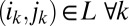 . If we presume that events take place on these edges in the order given, there is a unique temporal motif
  that corresponds to location
  . We take into account the structure of the aggregate network by modeling the motif count
  on
on  as a random variable under the null hypothesis
  that motif count at
  does not depend on node types.
What can the motif count depend on if not node types? There are two possible factors: the weights of the edges in  , and the network structure outside
  . We approximate the latter effect to be negligible: The occurrence of a motif on
  does not depend on events taking place on other edges. (The largest approximation comes from not taking into account events on adjacent edges that could render temporal subgraphs on
  invalid.)
Edge weights, however, are likely to correlate strongly with motif counts. Let  denote a sequence of edge weights in the aggregate network, and
  , the weight sequence of the edges in
  . Assuming
  is true and given the above approximation,
  is independent of node types and depends only on
  . We thus write
  , where
  is motif m without node types—in other words,
  follows a distribution parameterized by
  and
and  . The distributions
  are estimated from data. By summing over all locations for which
  , we obtain the total motif count under the null hypothesis:
 |
In SI Text, we present an algorithm for generating samples of  , and also prove that
  is an unbiased estimate of
  when
when  is true.
Because each distribution  is estimated from the data, large dataset is a necessity. In addition, edge weights for different nodes types should not be too disparate: If the edge weights are significantly higher for some node types,
  will be estimated using only these node types and therefore sampling will always produce
  . However, this means that the estimates produced by the null model are conservative, erring on the side of smaller effect. For the same reason, the results are not biased by rare high-weight edges: If there is only one location with weight sequence w, the distribution
  is a δ function and sampling will always produce
  .
.
Source Code.
The program used to enumerate temporal motifs and calculate the null model is available as free software: https://github.com/lkovanen/TMFinder.
Supplementary Material
Acknowledgments
We thank Albert-László Barabási of Northeastern University for providing access to the mobile phone dataset. The project ICTeCollective acknowledges financial support by the Future and Emerging Technologies (FET) program within the Seventh Framework Program for Research of the European Commission, under FET-Open Grant 238597. L.K. is supported by the Doctoral Program Brain and Mind. J.K. is partially supported by the Finland Distinguished Professor Program of Tekes. J.S. is supported by Academy of Finland Project 260427. We acknowledge the computational resources provided by Aalto Science-IT Project.
Footnotes
The authors declare no conflict of interest.
This article contains supporting information online at www.pnas.org/lookup/suppl/doi:10.1073/pnas.1307941110/-/DCSupplemental.
References
- 1.Borgatti SP, Mehra A, Brass DJ, Labianca G. Network analysis in the social sciences. Science. 2009;323(5916):892–895. doi: 10.1126/science.1165821. [DOI] [PubMed] [Google Scholar]
- 2.Wasserman S, Faust K. Social Network Analysis: Methods and Applications. Cambridge, UK: Cambridge Univ Press; 1994. [Google Scholar]
- 3.Kossinets G, Watts DJ. Empirical analysis of an evolving social network. Science. 2006;311(5757):88–90. doi: 10.1126/science.1116869. [DOI] [PubMed] [Google Scholar]
- 4.Lazer D, et al. Social science. Computational social science. Science. 2009;323(5915):721–723. doi: 10.1126/science.1167742. [DOI] [PMC free article] [PubMed] [Google Scholar]
- 5.Onnela J-P, et al. Structure and tie strengths in mobile communication networks. Proc Natl Acad Sci USA. 2007;104(18):7332–7336. doi: 10.1073/pnas.0610245104. [DOI] [PMC free article] [PubMed] [Google Scholar]
- 6. Ugander J, Karrer B, Backstrom L, Marlow C (2011) The anatomy of the Facebook social graph. arXiv:1111.4503.
- 7.Takhteyev Y, Gruzd A, Wellman B. Geography of Twitter networks. Soc Networks. 2012;34(1):73–81. [Google Scholar]
- 8.Fortunato S. Community detection in graphs. Phys Rep. 2010;486(3–5):75–174. [Google Scholar]
- 9.Bond RM, et al. A 61-million-person experiment in social influence and political mobilization. Nature. 2012;489(7415):295–298. doi: 10.1038/nature11421. [DOI] [PMC free article] [PubMed] [Google Scholar]
- 10.Braha D, Bar-Yam Y. In: Adaptive Networks: Theory, Models and Applications. Gross T, Sayama H, editors. Heidelberg: Springer; 2009. pp. 39–50. [Google Scholar]
- 11.Barabási A-L. The origin of bursts and heavy tails in human dynamics. Nature. 2005;435(7039):207–211. doi: 10.1038/nature03459. [DOI] [PubMed] [Google Scholar]
- 12.Wu Y, Zhou C, Xiao J, Kurths J, Schellnhuber HJ. Evidence for a bimodal distribution in human communication. Proc Natl Acad Sci USA. 2010;107(44):18803–18808. doi: 10.1073/pnas.1013140107. [DOI] [PMC free article] [PubMed] [Google Scholar]
- 13. Karsai M, Kaski K, Barabási AL, Kertész J (2012) Universal features of correlated bursty behaviour. Sci Rep 2:397. [DOI] [PMC free article] [PubMed]
- 14.Malmgren RD, Stouffer DB, Motter AE, Amaral LAN. A Poissonian explanation for heavy tails in e-mail communication. Proc Natl Acad Sci USA. 2008;105(47):18153–18158. doi: 10.1073/pnas.0800332105. [DOI] [PMC free article] [PubMed] [Google Scholar]
- 15.Karsai M, et al. Small but slow world: How network topology and burstiness slow down spreading. Phys Rev E Stat Nonlin Soft Matter Phys. 2011;83(2 Pt 2):025102. doi: 10.1103/PhysRevE.83.025102. [DOI] [PubMed] [Google Scholar]
- 16.Miritello G, Moro E, Lara R. Dynamical strength of social ties in information spreading. Phys Rev E Stat Nonlin Soft Matter Phys. 2011;83(4 Pt 2):045102. doi: 10.1103/PhysRevE.83.045102. [DOI] [PubMed] [Google Scholar]
- 17.Jo H-H, Karsai M, Kertész J, Kaski K. Circadian pattern and burstiness in human communication activity. New J Phys. 2012;14(1):013055. [Google Scholar]
- 18.Iribarren JL, Moro E. Impact of human activity patterns on the dynamics of information diffusion. Phys Rev Lett. 2009;103(3):038702. doi: 10.1103/PhysRevLett.103.038702. [DOI] [PubMed] [Google Scholar]
- 19.Jiang Z-Q, et al. Calling patterns in human communication dynamics. Proc Natl Acad Sci USA. 2013;110(5):1600–1605. doi: 10.1073/pnas.1220433110. [DOI] [PMC free article] [PubMed] [Google Scholar]
- 20.Kandel DB. Homophily, selection, and socialization in adolescent friendships. Am J Sociol. 1978;84(2):427–436. [Google Scholar]
- 21.Moody J. Race, school integration, and friendship segregation in America. Am J Sociol. 2001;107(3):679–716. [Google Scholar]
- 22.McPherson M, Smith-Lovin L, Cook JM. Birds of a feather: Homophily in social networks. Annu Rev Sociol. 2001;27(1):415–444. [Google Scholar]
- 23. Leskovec J, Horvitz E (2008) Planetary-scale views on a large instant-messaging network. Proceedings of the 17th International Conference on World Wide Web, WWW ’08 (ACM, New York), pp 915–924.
- 24.Lewis K, Kaufman J, Gonzalez M, Wimmer A, Christakis N. Tastes, ties, and time: A new social network dataset using Facebook.com. Soc Networks. 2008;30(4):330–342. [Google Scholar]
- 25.Smoreda Z, Licoppe C. Gender-specific use of the domestic telephone. Soc Psychol Q. 2000;63(3):238–252. [Google Scholar]
- 26.Palchykov V, Kaski K, Kertész J, Barabási A-L, Dunbar RIM. Sex differences in intimate relationships. Sci Rep. 2012;2:370. doi: 10.1038/srep00370. [DOI] [PMC free article] [PubMed] [Google Scholar]
- 27.Holme P, Saramäki J. Temporal networks. Phys Rep. 2012;519(3):97–125. [Google Scholar]
- 28.Kovanen L, Karsai M, Kaski K, Kertész J, Saramäki J. Temporal motifs in time-dependent networks. J Stat Mech. 2011;2011(11):P11005. [Google Scholar]
- 29.Granovetter M. The strength of weak ties. Am J Sociol. 1973;78(6):1360–1380. [Google Scholar]
- 30.Milo R, et al. Network motifs: Simple building blocks of complex networks. Science. 2002;298(5594):824–827. doi: 10.1126/science.298.5594.824. [DOI] [PubMed] [Google Scholar]
- 31.Shen-Orr SS, Milo R, Mangan S, Alon U. Network motifs in the transcriptional regulation network of Escherichia coli. Nat Genet. 2002;31(1):64–68. doi: 10.1038/ng881. [DOI] [PubMed] [Google Scholar]
- 32.Artzy-Randrup Y, Fleishman SJ, Ben-Tal N, Stone L. Comment on “Network motifs: Simple building blocks of complex networks” and “Superfamilies of evolved and designed networks”. Science. 2004;305(5687):1107. doi: 10.1126/science.1099334. author reply 1107. [DOI] [PubMed] [Google Scholar]
- 33.Onnela J-P, Saramäki J, Kertész J, Kaski K. Intensity and coherence of motifs in weighted complex networks. Phys Rev E Stat Nonlin Soft Matter Phys. 2005;71(6 Pt 2):065103. doi: 10.1103/PhysRevE.71.065103. [DOI] [PubMed] [Google Scholar]
- 34.Ciriello G, Guerra C. A review on models and algorithms for motif discovery in protein–protein interaction networks. Brief Funct Genomics Proteomics. 2008;7(2):147–156. doi: 10.1093/bfgp/eln015. [DOI] [PubMed] [Google Scholar]
- 35.Friston K. Ten ironic rules for non-statistical reviewers. Neuroimage. 2012;61(4):1300–1310. doi: 10.1016/j.neuroimage.2012.04.018. [DOI] [PubMed] [Google Scholar]
- 36.Palla G, Derényi I, Farkas I, Vicsek T. Uncovering the overlapping community structure of complex networks in nature and society. Nature. 2005;435(7043):814–818. doi: 10.1038/nature03607. [DOI] [PubMed] [Google Scholar]
- 37.Vazquez A, Rácz B, Lukács A, Barabási A-L. Impact of non-Poissonian activity patterns on spreading processes. Phys Rev Lett. 2007;98(15):158702. doi: 10.1103/PhysRevLett.98.158702. [DOI] [PubMed] [Google Scholar]
- 38.Schneider CM, Belik V, Couronné T, Smoreda Z, González MC. Unravelling daily human mobility motifs. J R Soc Interface. 2013;10(84):20130246. doi: 10.1098/rsif.2013.0246. [DOI] [PMC free article] [PubMed] [Google Scholar]
Associated Data
This section collects any data citations, data availability statements, or supplementary materials included in this article.