MODEL-BASED MR PARAMETER MAPPING WITH SPARSITY CONSTRAINT

Abstract

MR parameter mapping (e.g., T₁ mapping, T₂ mapping, or $T_2^{*}$ mapping) is a valuable tool for tissue characterization. However, its practical utility has been limited due to long data acquisition time. This paper addresses this problem with a new model-based parameter mapping method, which utilizes an explicit signal model and imposes a sparsity constraint on the parameter values. The proposed method enables direct estimation of the parameters of interest from highly undersampled, noisy k-space data. An algorithm is presented to solve the underlying parameter estimation problem. Its performance is analyzed using estimation-theoretic bounds. Some representative results from T₂ brain mapping are also presented to illustrate the performance of the proposed method for accelerating parameter mapping.

1. INTRODUCTION

MR parameter mapping (e.g., T₁ mapping, T₂ mapping, and $T_2^{*}$ mapping) often involves collecting a sequence of images {I_m (x) } with variable parameter-weightings. The parameter-weighted images I_m(x) are related to the measured k-space data by

$$d_m(\mathbf{k})=\int I_m(\mathbf{x})\text{exp}(-i2\pi \mathbf{k}·\mathbf{x})d\mathbf{x}+n_m(\mathbf{k})$$ (1)

where n_m(k) denotes complex white Gaussian noise. Conventional parameter mapping methods sample k-space at the Nyquist rate in the acquisition of each d_m(k) from which the I_m(x) are reconstructed, which are followed by parameter estimation from I_m(x). One major practical limitation of these parameter mapping methods is long data acquisition time. To alleviate this problem, a number of methods have been proposed to enable parameter mapping from undersampled data. One approach to parameter mapping with sparse sampling is to reconstruct I_m(x) from undersampled data using various constraints (e.g., sparsity constraint [1] or partial separability constraint (PS) [2]), which is followed by parameter estimation from I_m(x). Several successful examples of this approach are described in [3–7]. Another approach is to directly estimate the parameter map from the undersampled k-space data, bypassing the image reconstruction step completely [8–10]. This approach formulates the parameter mapping problem as a statistical parameter estimation problem, which allows for easier performance characterization. Our proposed method uses this approach but also allows sparsity constraint to be effectively used for improved parameter estimation. The advantages of using the sparsity constraint in this context are analyzed theoretically and demonstrated empirically in this paper.

The rest of paper is organized as follows: Section 2 describes the proposed method in detail, including problem formulation, optimization algorithm, and estimation-theoretic characterization; Section 3.1 illustrates the potential benefits of applying sparsity constraint directly to the parameter domain with an example of T₂ brain mapping; Section 4 contains the conclusion of the paper.

2. PROPOSED METHOD

We assume that the parameter-weighted image sequence consists of M image frames, for each of which, a finite number of measurements, denoted as d_m ∈ ℂ ^P_m, are collected. For convenience, we use a discrete image model, in which I_m is an N × 1 vector. In this setting, the imaging equation (1) can be written as

$${\mathbf{d}}_m={\mathbf{F}}_m{\mathbf{I}}_m+{\mathbf{n}}_m,$$ (2)

m = 1, … , M, where F_m ∈ ℂ^P_m×N denotes the Fourier encoding matrix, and n_m ∈ ℂ^P_m denotes the complex white Gaussian noise with variance σ².

2.1. Problem Formulation

2.1.1. Signal model

In parameter mapping, the parameter-weighted images I_m(x) can be written as [8–10]

$$I_m(\mathbf{x})=\rho (\mathbf{x})\varphi (\theta (\mathbf{x}),{\mathbf{\gamma }}_m),$$ (3)

where ρ(x) represents the spin density distribution, θ(x) is the desired parameter map (e.g., T₁-map, T₂-map, or $T_2^{*}$-map), and γ_m contains the user-specified parameters for a given data acquisition sequence (e.g., echo time T_E, repetition time T_R, flip angle α, etc.). The exact mathematical form of (3) is known for a chosen parameter mapping experiment. For example, for a variable flip angle T₁-mapping experiment, (3) can be written as

$$I_m(\mathbf{x})=\rho (\mathbf{x})\frac{\text{sin}{\alpha }_m(1-e^{-T_R/T_1(\mathbf{x})})}{1-\text{cos}{\alpha }_m{e}^{-T_R/T_1(\mathbf{x})}},$$ (4)

where T₁(x) is the parameter map of interest, α_m and T_R are pre-selected data acquisition parameters. We can, therefore, assume that ϕ is a known function in (3). After discretization, it can be written as

$${\mathbf{I}}_m={\mathbf{\Phi }}_m(\mathbf{\theta })\mathbf{\rho },$$ (5)

where Φ_m ∈ ℂ^{N × N} is a diagonal matrix with [Φ_m]_n,n = ϕ(θ_n, γ_m), θ_n denotes the parameter value at the nth voxel, and ρ ∈ ℂ^{N × 1} contains the spin density values. Note that in (5), I_m linearly depends on ρ, but nonlinearly depends on θ.

Substituting (5) into (2) yields the following observation model

$${\mathbf{d}}_m={\mathbf{F}}_m{\mathbf{\Phi }}_m(\mathbf{\theta })\mathbf{\rho }+{\mathbf{n}}_m.$$ (6)

We can determine θ and ρ from the measured data, {d_m}, directly based on (6) without reconstructing {I_m(x)}. Under the assumption that n_m are white Gaussian noise, the maximum likelihood (ML) estimate of ρ and θ is given by [8–10]

$$\{{\mathbf{\rho ̂}}_{\mathrm{M}\mathrm{L}},{\mathbf{\theta ̂}}_{\mathrm{M}\mathrm{L}}\}=\underset{\mathbf{\rho },\mathbf{\theta }}{\text{argmin}}\sum _{m=1}^M{\Vert {\mathbf{d}}_m-{\mathbf{F}}_m{\mathbf{\Phi }}_m(\mathbf{\theta })\mathbf{\rho }\Vert }_2^2.$$ (7)

This is a standard nonlinear least squares problem, which can be solved using a number of numerical algorithms [11], although it may have multiple local minima.

2.1.2. Sparsity constraint

It is well known that in parameter mapping, the values of θ are tissue-dependent. Since the number of tissue types is relatively small compared to the number of voxels, we can apply a sparsity constraint to θ with an appropriate sparsifying transform. Incorporating the sparsity constraint into the ML estimation framework in (7) yields:

$$\{{\mathbf{\rho ̂}}_{\mathrm{s}\mathrm{M}\mathrm{L}},{\mathbf{\theta ̂}}_{\mathrm{s}\mathrm{M}\mathrm{L}}\}=\underset{\mathbf{\rho },\mathbf{\theta }}{\text{argmin}}\sum _{m=1}^M{\Vert {\mathbf{d}}_m-{\mathbf{F}}_m{\mathbf{\Phi }}_m(\mathbf{\theta })\mathbf{\rho }\Vert }_2^2,\mathrm{s}.\mathrm{t}.{\Vert \mathbf{W}\mathbf{\theta }\Vert }_0\le K,$$ (8)

where W is a chosen sparsifying transform (e.g., wavelet transform), ∥·∥₀ represents the ℓ₀ pseudo norm, and K is a given sparsity level. For simplicity, we assume that W is an orthonormal transform in this paper. Under this assumption, we can solve the following equivalent formulation:

$$\{{\mathbf{\rho ̂}}_{\mathrm{s}\mathrm{M}\mathrm{L}},{\mathbf{ĉ}}_{\mathrm{s}\mathrm{M}\mathrm{L}}\}=\underset{\mathbf{\rho },\mathbf{c}}{\text{argmin}}\sum _{m=1}^M{\Vert {\mathbf{d}}_m-{\mathbf{F}}_m{\mathbf{\Phi }}_m({\mathbf{W}}^H\mathbf{c})\mathbf{\rho }\Vert }_2^2,\mathrm{s}.\mathrm{t}.{\Vert \mathbf{c}\Vert }_0\le K,$$ (9)

where c = W θ contains the transform domain coefficients.

2.2. Optimization Algorithm

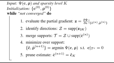
We present a practical and efficient algorithm to solve (9). Note that (9) is a nonlinear optimization problem with a smooth, non-convex cost function and an explicit sparsity constraint. A number of greedy pursuit algorithms have recently been developed to address this type of problems (e.g., [12–14]). These algorithms are mostly generalizations of greedy algorithms for compressive sensing with linear measurements. Here we adapt one efficient algorithm, the Gradient Support Pursuit (GraSP) algorithm [14], to solve (9).

GraSP is an iterative algorithm that utilizes the gradient of the cost function to identify the candidate support of the sparse coefficients, and then solves the nonlinear optimization problem constrained to the identified support. Specifically, the procedure for solving (9) can be summarized in Algorithm 1. We denote the cost function in (9) as Ψ(c, ρ), and the solution at the nth iteration as

Algorithm 1.

The Gra SP Algorithm for Solving (9).

{ ĉ⁽ⁿ⁾,ρ̂⁽ⁿ⁾}. At the (n+1)th iteration, we first compute the partial derivative of Ψ with respect to c at { ĉ⁽ⁿ⁾,ρ̂⁽ⁿ⁾}:

$$\mathbf{z}=\frac{\partial \mathrm{\Psi }}{\partial \mathbf{c}}=\mathbf{W}\sum _{m=1}^M\frac{\partial {\mathbf{\Phi }}_m}{\partial \mathbf{\theta }}\mathrm{R}\mathrm{e}\{{\mathbf{F}}_m^H[{\mathbf{F}}_m{\mathbf{\Phi }}_m(\mathbf{\theta })\mathbf{\rho }-{\mathbf{d}}_m]\},$$ (10)

where $\frac{\partial {\mathbf{\Phi }}_m}{\partial \mathbf{\theta }}$ is a diagonal matrix with ${\left[\frac{\partial {\mathbf{\Phi }}_m}{\partial \mathbf{\theta }}\right]}_{n,n}=\frac{\partial \varphi ({\mathbf{\theta }}_n,{\mathbf{\gamma }}_m)}{\partial {\mathbf{\theta }}_n}.$ Secondly, we identify a support set Ƶ associated with the 2K largest entries of z, i.e., Ƶ = supp(z_2K) (Intuitively, minimization over Ƶ would lead to the most effective reduction in the cost function value). Then we merge Ƶ with supp(ĉ⁽ⁿ⁾) to form a combined support set Ƭ , over which we minimize Ψ. Finally, after obtaining the solution c̃, we only keep its largest K entries and set other entries to zero, i.e., ĉ⁽ⁿ⁺¹⁾ = c̃_K. The above procedure is repeated until the relative change between two consecutive iterations is smaller than some pre-specified threshold.

The algorithm is computationally efficient: at each iteration it only involves gradient evaluation and the solution of a support constrained problem. For the support-constrained optimization problem, its computational complexity is much smaller than (7) due to the reduced number of unknowns. It has been shown in [14] that under certain theoretical conditions (the generalization of restricted isometry property in linear measurement model), GraSP has guaranteed convergence. However, note that verifying these theoretical conditions for a specific problem is typically NP-hard. In solving (9), we estimate the initial solution {c⁽⁰⁾, ρ⁽⁰⁾} from a low-resolution image sequence, which have consistently yielded good empirical results.

2.3. Estimation-Theoretic Characterization

The formulation (8) or (9) performs parameter estimation with sparsity constraint. In this subsection, we derive the sparsity-constrained Cramer-Rao lower bound (CRLB) [15,16] on θ, which provides useful insights into the benefits of incorporating the sparsity constraint into the parameter estimation problem. Furthermore, it can also be used as a benchmark to evaluate our solution algorithm.

We first derive the sparsity-constrained CRLB on c, from which we can obtain a bound on θ. Assume that c is K-sparse, i.e., c ∈Ω = {c ∈ ℝ^N supp(c) ≤ K} and K is given. Based on (6) and c = Wθ, the sparsity constrained CRLB for any locally unbiased estimator ĉ can be expressed as

$$\text{Cov}(\mathbf{ĉ})\ge {\mathbf{Z}}_{\mathrm{s}},$$ (11)

where

$${\mathbf{Z}}_{\mathrm{s}}=[{\mathbf{E}}_N{\mathbf{0}}_N]\mathbf{A}{({\mathbf{A}}^T\mathbf{J}\mathbf{A})}^{†}{\mathbf{A}}^T\left[\begin{array}{c}{\mathbf{E}}_N\hfill \\ {\mathbf{0}}_N\hfill \end{array}\right]\in {ℝ}^{N\times N},$$ (12)

J ∈ ℝ^{2N × 2N} is the Fisher information matrix (FIM), $\mathbf{A}=\left[\begin{array}{cc}{\mathbf{Ẽ}}_K\hfill & \mathbf{0}\hfill \\ \mathbf{0}\hfill & {\mathbf{E}}_N\hfill \end{array}\right]$, E_N is the N × N identity matrix, Ẽ_K is an N × K sub-matrix of E_N whose columns are selected based on the support of c. We can simplify the expression of Z_s in (12). Let the partitioned FIM be $\mathbf{J}=\left[\begin{array}{cc}{\mathbf{J}}_{\mathbf{c},\mathbf{c}}\hfill & {\mathbf{J}}_{\mathbf{c},\mathbf{\rho }}\hfill \\ {\mathbf{J}}_{\mathbf{\rho },\mathbf{c}}\hfill & {\mathbf{J}}_{\mathbf{\rho },\mathbf{\rho }},\hfill \end{array}\right]\text{and}{\mathbf{A}}^T\mathbf{J}\mathbf{A}=\left[\begin{array}{cc}{\mathbf{G}}_{11}\hfill & {\mathbf{G}}_{12}\hfill \\ {\mathbf{G}}_{21}\hfill & {\mathbf{G}}_{22}\hfill \end{array}\right],$ where ${\mathbf{G}}_{11}={\mathbf{Ẽ}}_K^T{\mathbf{J}}_{\mathbf{c}\mathbf{c}}{\mathbf{Ẽ}}_K,{\mathbf{G}}_{12}={\mathbf{Ẽ}}_K^T{\mathbf{J}}_{\mathbf{c}\mathbf{\rho }},{\mathbf{G}}_{21}={\mathbf{G}}_{12}^T,$ and G₂₂ = J_{ρ ρ}. Using the pseudo-inverse of the partitioned Hermitian matrix [17], it can be shown that¹

$${\mathbf{Z}}_{\mathrm{s}}={\mathbf{Ẽ}}_K({\mathbf{G}}_{11}^{†}+{\mathbf{G}}_{11}^{†}{\mathbf{G}}_{12}{\mathbf{Q}}_{\mathbf{s}}^{†}{\mathbf{G}}_{21}{\mathbf{G}}_{11}^{†}){\mathbf{Ẽ}}_K^T,$$ (13)

where ${\mathbf{Q}}_s={\mathbf{G}}_{22}-{\mathbf{G}}_{21}{\mathbf{G}}_{11}^{†}{\mathbf{G}}_{12}.$

With θ̂ = W^H ĉ, the bound on θ̂ can be written as

$$\text{Cov}(\mathbf{\theta ̂}\text{)}\ge {\mathbf{W}}^H{\mathbf{Z}}_s\mathbf{W}.$$ (14)

Taking the diagonal entries of the covariance matrix, we can obtain the bound on the variance of θ̂ at each voxel as

$$\text{Var}({\mathbf{\theta ̂}}_n\text{)}\ge {[{\mathbf{W}}^H{\mathbf{Z}}_s\mathbf{W}]}_{n,n}.$$ (15)

Under the assumption that θ̂_sML is locally unbiased in (8), the righthand side of (14) also provides a lower bound on Cov(θ̂_sML). Note that this assumption can approximately hold with a finite number of measurements and a reasonable signal-to-noise ratio.

Excluding the sparsity constraint, we can calculate the unconstrained CRLB as follows:

$$\text{Cov}(\mathbf{\theta ̂}\text{)}\ge {\mathbf{W}}^H\mathbf{Z}\mathbf{W},$$ (16)

where $\mathbf{Z}=({\mathbf{J}}_{\mathbf{c},\mathbf{c}}^{†}+{\mathbf{J}}_{\mathbf{c},\mathbf{c}}^{†}{\mathbf{J}}_{\mathbf{c},\mathbf{\rho }}{\mathbf{Q}}^{†}{\mathbf{J}}_{\mathbf{\rho },\mathbf{c}}{\mathbf{J}}_{\mathbf{c},\mathbf{c}}^{†})$ and $\mathbf{Q}={\mathbf{J}}_{\mathbf{\rho },\mathbf{\rho }}-{\mathbf{J}}_{\mathbf{\rho },\mathbf{c}}{\mathbf{J}}_{\mathbf{c},\mathbf{c}}^{†}{\mathbf{J}}_{\mathbf{c},\mathbf{\rho }}.$ It has been shown in [15, 16] that W^HZW ≥ W^HZ_sW. Therefore, incorporating sparsity constraint can be theoretically demonstrated to be beneficial. In the next section, we will calculate the above bounds in a numerical brain phantom to illustrate the potential benefits of using the sparsity constraint in (8).

3. RESULTS

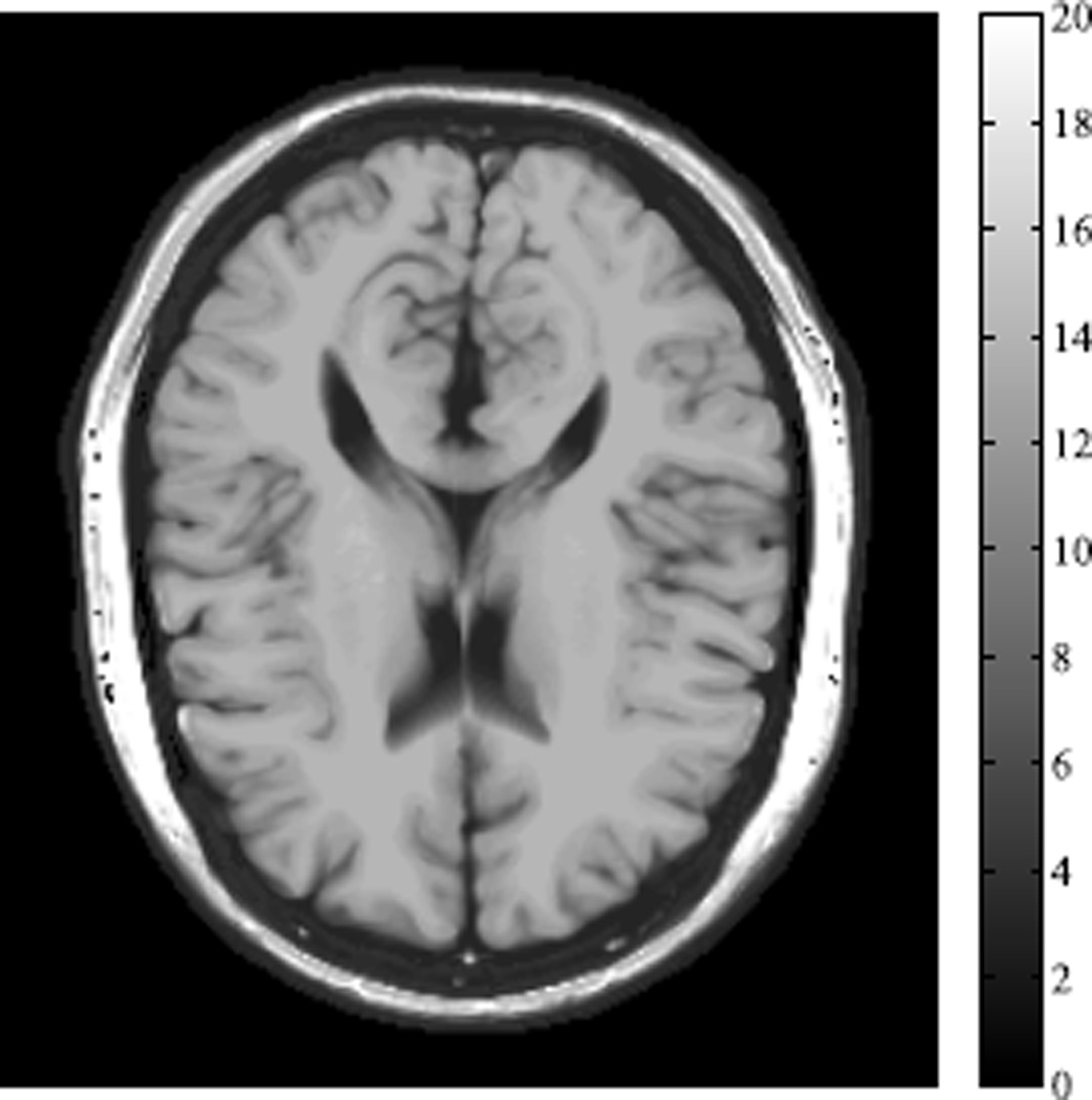
In this section, we use a T₂ mapping example with a numerical brain phantom [18] to illustrate the estimation-theoretic bounds and empirical performance of the proposed method. In this example, ϕ(θ, γ_m) = exp(−γ_mR₂), where R₂ is the relaxation rate (i.e., the reciprocal of T₂), and γ_m = T_E,m is the echo time. The R₂ map of the brain phantom is illustrated in Fig. 1. We used a multi-echo spin echo acquisition with a total number of 16 echoes and 10 ms echo spacing. We define the acceleration factor (AF) as $NM/({\sum }_{m=1}^M{P}_m),$ and the signal to noise ratio (SNR) as the ratio of the signal intensity (in a region of the white matter) to the noise standard deviation.

Fig. 1.

The R₂ map of the numerical brain phantom.

3.1. Performance Bounds

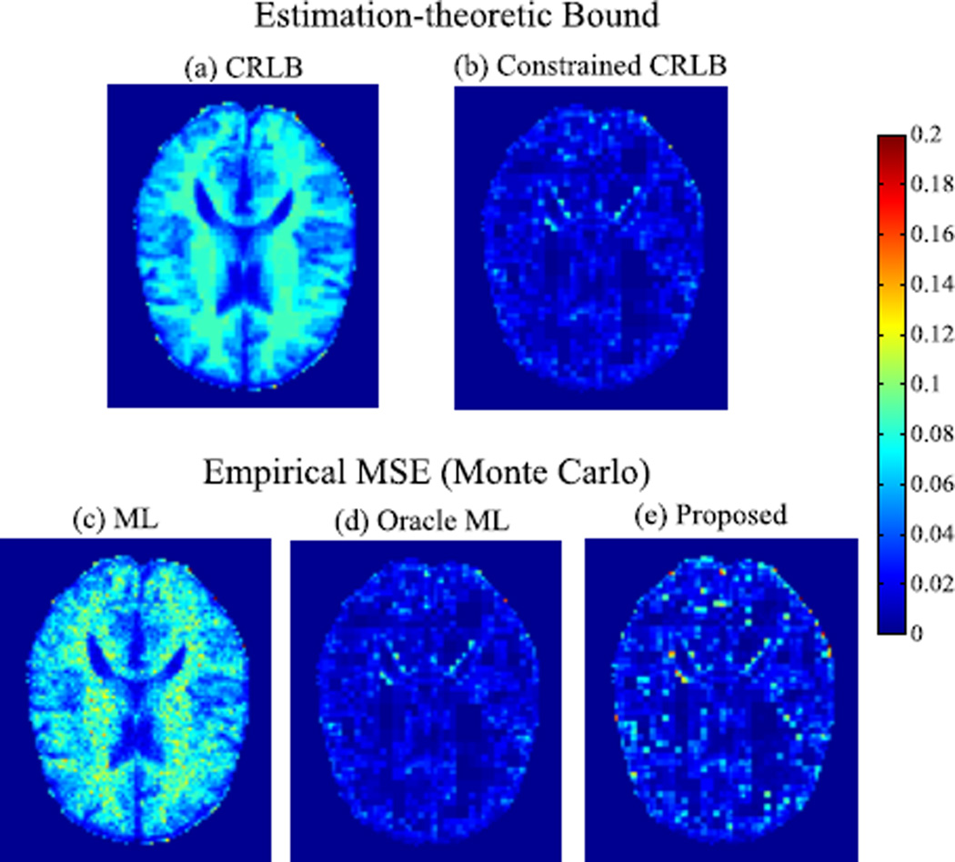
We compute the estimation-theoretic bounds in (14) and (16) to analyze the potential benefits of incorporating the sparsity constraint. Specifically, we take the diagonal entries of the covariance matrix to extract the bounds on the variances for each voxel. We simulated a data set that has 1) a mono-exponential signal model, and 2) a R₂ map that is sparse in the wavelet domain². Data acquisition was performed at AF = 4 and SNR = 28dB. To reduce the memory burden, we resized the original brain phantom to a smaller scale.

In addition to evaluating the performance bounds, we also performed a Monte Carlo study (with 300 trials) to compute the empirical MSE of the ML estimator in (7) and the proposed estimator in (9), respectively. The true sparsity level was used to set the parameter K for (9). Furthermore, we considered an oracle ML estimator that assumes complete knowledge of the exact sparse support of the R₂ map. The MSE of the proposed estimator in (8) should be bounded below by that of the oracle estimator.

The performance bound and empirical MSE³ are shown in Fig.2. As can be seen, the CRLB varies with respect to different brain tissues. With the wavelet domain sparsity constraint, the constrained CRLB is significantly lower than the CRLB and it becomes much less tissue-dependent. The theoretical prediction matches well with the simulation results. The proposed method yields much lower MSE than the ML estimator, demonstrating again the benefits of introducing the sparsity constraint for improving parameter estimation. Note that the performance of the proposed method is very close to that of the oracle estimator, which matches well with the constrained CRLB.

Fig. 2.

Estimation-theoretic bounds and empirical MSE of the ML, oracle ML, and proposed estimators. Note that the background, skull, and the scalp are are not region of interest for our study, and thus they were set to zero.

3.2. Empirical performance

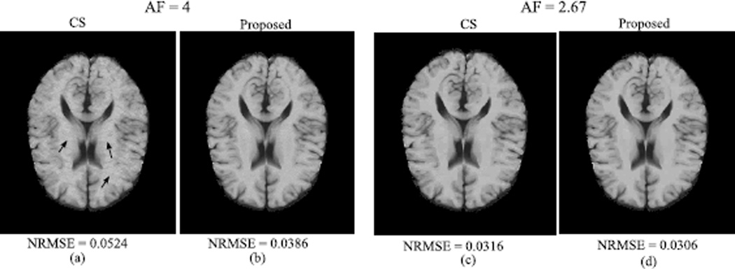
To demonstrate the empirical performance of the proposed method, we simulated the phantom in a way that both signal model mismatch (multi-exponential model caused by partial volume effect) and sparsity model mismatch (wavelet coefficients are approximately sparse) exist. We acquired two sets of k-space measurements at AF = 2.67 and 4, both of which had SNR = 24dB. Here, we manually chose the sparsity level K = 0.2N for the proposed method. Note that selecting K in a more principled way is worth of further study.

We compared the proposed method with a dictionary learning-based compressed sensing reconstruction [3] (referred to as CS), which only takes into account the temporal relaxation process. The reconstructed R₂ maps are shown in Fig.3, along with the normalized root-mean-square-error (NRMSE) listed below the reconstructions. As can be seen, when AF = 4, the CS reconstruction shows several artifacts (marked by arrows), although these artifacts were significantly reduced at the lower AF. In contrast, the proposed method produced higher-quality parameter maps at both high and low acceleration levels. The observations are consistent with the values of NRMSE.

Fig. 3.

(a)–(b) Reconstructed R₂ maps at AF = 4; (c)–(d) Reconstructed R₂ maps at AF = 2.67.

4. CONCLUSION

This paper presented a new method to directly reconstruct parameter maps from highly undersampled, noisy k-space data, utilizing an explicit signal model while imposing a sparsity constraint on the parameter values. A greedy pursuit algorithm was described to solve the underlying optimization problem. The benefit of incorporating sparsity constraint is analyzed theoretically using estimation-theoretic bounds and also illustrated empirically in a T₂ mapping example. The proposed method should prove useful for fast MR parameter mapping with sparse sampling.

REFERENCES

- 1.Lustig M, Donoho D, Pauly JM. Sparse MRI: The application of compressed sensing for rapid MR imaging. Magn. Reson. Med. 2007;58:1182–1195. doi: 10.1002/mrm.21391. [DOI] [PubMed] [Google Scholar]
- 2.Liang Z-P. Spatiotemporal imaging with partially separable functions. Proc. IEEE Int. Symp. Biomed. Imaging. 2007:988–991. [Google Scholar]
- 3.Doneva M, Bornert P, Eggers H, Stehning C, Senegas J, Mertins A. Compressed sensing reconstruction for magnetic resonance parameter mapping. Magn. Reson. Med. 2010;64:1114–1120. doi: 10.1002/mrm.22483. [DOI] [PubMed] [Google Scholar]
- 4.Feng L, Otazo R, Jung H, Jensen JH, Ye JC, Sodickson DK, Kim D. Accelerated cardiac T2 mapping using breath-hold multiecho fast spin-echo pulse sequence with k-t FOCUSS. Magn. Reson. Med. 2011;65(6):1661–1669. doi: 10.1002/mrm.22756. [DOI] [PMC free article] [PubMed] [Google Scholar]
- 5.Petzschner FH, Ponce IP, Blaimer M, Jakob PM, Breuer FA. Fast MR parameter mapping using k-t principal component analysis. Magn. Reson. Med. 2011;66:706–716. doi: 10.1002/mrm.22826. [DOI] [PubMed] [Google Scholar]
- 6.Huang C, Graff CG, Clarkson EW, Bilgin A, Altbach MI. T2 mapping from highly undersampled data by recon- struction of principal component coefficient maps using compressed sensing. Magn. Reson. Med. 2012;67(5):1355–1366. doi: 10.1002/mrm.23128. [DOI] [PMC free article] [PubMed] [Google Scholar]
- 7.Zhao B, Lu W, Liang Z-P. Highly accelerated parameter mapping with joint partial separability and sparsity constraints. Proc. Int. Symp. Magn. Reson. Med. 2012:2233. [Google Scholar]
- 8.Haldar JP, Hernando D, Liang Z-P. Super-resolution reconstruction of MR image sequences with contrast modeling. Proc. IEEE Int. Symp. Biomed. Imaging. 2009:266–269. [Google Scholar]
- 9.Block K, Uecker M, Frahm J. Model-based iterative reconstruction for radial fast spin-echo MRI. IEEE Trans. Med Imaging. 2009;28:1759–1769. doi: 10.1109/TMI.2009.2023119. [DOI] [PubMed] [Google Scholar]
- 10.Sumpf TJ, Uecker M, Boretius S, Frahm J. Model-based nonlinear inverse reconstruction for T2 mapping using highly undersampled spin-echo MRI. J Magn Reson Imaging. 2011;34:420–428. doi: 10.1002/jmri.22634. [DOI] [PubMed] [Google Scholar]
- 11.Nocedal J, Wright SJ. Numerical Optimization. (2nd Edition) New York: NY: Springer; 2006. [Google Scholar]
- 12.Beck A, Eldar YC. Sparsity constrained nonlinear optimization: Optimality conditions and algorithms. 2012 preprint. [Google Scholar]
- 13.Blumensath T. Compressed sensing with nonlinear observations and related nonlinear optimization problems. 2012 preprint. [Google Scholar]
- 14.Bahmani S, Raj B, Boufounos P. Greedy sparsity-constrained optimization. 2012 preprint. [Google Scholar]
- 15.Gorman JD, Hero AO. Lower bounds for parametric estimation with constraints. IEEE Trans. Inf. Theory. 1990;(6):1285–1301. [Google Scholar]
- 16.Ben-Haim Z, Eldar YC. The Cramer-Rao bound for es- timating a sparse parameter vector. IEEE Trans. Signal Process. 2010;(6):3384–3389. [Google Scholar]
- 17.Rohde CA. Generalized inverses of partitioned matrices. J. Soc. Indust. Appl. Math. 1965;13:1033–1035. [Google Scholar]
- 18.Collins DL, Zijdenbos AP, Kollokian V, Sled JG, Kabani NJ, Holmes CJ, Evans AC. Design and construction of a realistic digital brain phantom. IEEE Trans. Med Imaging. 1998;17:463–468. doi: 10.1109/42.712135. [DOI] [PubMed] [Google Scholar]