Promoter-mediated Transcriptional Dynamics

Abstract

Genes in eukaryotic cells are typically regulated by complex promoters containing multiple binding sites for a variety of transcription factors, but how promoter dynamics affect transcriptional dynamics has remained poorly understood. In this study, we analyze gene models at the transcriptional regulation level, which incorporate the complexity of promoter structure (PS) defined as transcriptional exits (i.e., ON states of the promoter) and the transition pattern (described by a matrix consisting of transition rates among promoter activity states). We show that multiple exits of transcription are the essential origin of generating multimodal distributions of mRNA, but promoters with the same transition pattern can lead to multimodality of different modes, depending on the regulation of transcriptional factors. In turn, for similar mRNA distributions in the models, the mean ON or OFF time distributions may exhibit different characteristics, thus providing the supplemental information on PS. In addition, we demonstrate that the transcriptional noise can be characterized by a nonlinear function of mean ON and OFF times. These results not only reveal essential characteristics of promoter-mediated transcriptional dynamics but also provide signatures useful for inferring PS based on characteristics of transcriptional outputs.

Introduction

Gene expression involves transcription, translation, chromatin remodeling, histone modifications, alternative splicing, and recruitment of transcription factors (TFs), and polymerases. These biochemical processes inevitably lead to stochastic fluctuations (or the noise) in expression levels (1–4). This noise is essential for many cellular functions (5,6) and has been identified as a key factor underlying the observed phenotypic variability of genetically identical cells in homogeneous environments (7). Although recent advances in experimental methods allow direct observations of real-time fluctuations in gene expression levels in individual live cells (8–12), there is considerable interest in theoretically understanding how different molecular mechanisms of gene expression affect variations in mRNA and protein levels across a population of cells. Quantifying the contributions of different sources of noise using stochastic models of gene expression is an important step toward understanding fundamental cellular processes and variations in cell populations (13–30).

Transcription is a key step during gene expression, where the transcription machinery is responsible for transcribing DNA to RNA and initiating mRNA transcripts (31). Biochemical processes associated with transcription often involve a variety of TFs, which bind to multiple sites on regulatory DNA in response to intracellular or extracellular signals. When bound to these sites, the TFs either inhibit or enhance transcription through interactions with RNA polymerase and other TFs. Most regulatory sequences called as “promoters” contain several operator sequences, each of which is often recognized with different affinities by more than one type of TF. For bacterial cells, the promoters that are viewed as simple can exist in a surprisingly large number of regulatory states. For example, the PRM promoter of phage lambda in E. coli is regulated by two different TFs binding to two sets of three operators that can be brought together by looping out the intervening DNA. As a result, the number of regulatory states of the PRM promoter is 128 (32). In contrast, eukaryotic promoters are more complex, involving nucleosomes competing with or being removed by TFs (33). In addition to the conventional regulation by TFs, the eukaryotic promoters can be also epigenetically regulated via histone modifications (34–36). Such regulation may lead to very complex promoter structure (PS) (37). To help readers understand how a PS is formed, we simply introduce three molecular mechanisms (38): 1) nucleosome occupancy that promoter-DNA condensation into chromatin may lead to long-lived, silenced or OFF, promoter states, which are followed by rapid, short-lived initiation events; 2) TATA box that activates the promoter by helping assemble the pre-initiation complex; 3) TF binding sites for which the molecular mechanism has not been well understood.

Transcription takes place often in a bursting manner. Single-cell experimental measurements have provided evidence for transcriptional bursting both in bacteria (8) and in eukaryotic cells (9,39). Although the sources of the transcriptional burst remain poorly understood (40), several lines of evidence (3,4,10,11,41–45) point to transitions among the ON and OFF states of the promoter as an important source of noise in gene expression, which is responsible for generating cell-to-cell heterogeneity in the response of genetically identical cells to the same stimulus. Complex promoters with more than two activity states are not the exception but the rule as combinatorial control of gene regulation by multiple TFs is widespread (46). In two relevant studies, an experiment in yeast cells demonstrated that high levels of cell-to-cell variability, originated by promoter state fluctuations, may confer cell colonies with an enhanced probability of cell survival when subjected to external stress (47); another experiment showed that a stable transcription scaffold that regulates the rate of transitions between ON and OFF states of the promoter can result in “bursts” of gene expression beneficial to increasing cell-to-cell variability (5). In particular, all three of the molecular mechanisms (described above) for the formation of PS can lead to transcriptional bursting. In fact, rapid, short-lived initiation events taking place in nucleosome occupancy can lead to bursting synthesis of mRNA (4); in the TATA box case, it was experimentally demonstrated that mutations that weaken the strength of the TATA box of the PHO5 gene in yeast cells result in a reduction in gene expression noise (4); in the case of TF binding sites, experiments have shown that the number of binding sites for TFs can significantly affect the gene expression noise (10,48).

Given the complexity of most PSs, quantitative models play an important role in testing molecular mechanisms of transcriptional regulation, helping to connect these biochemical models of transcription with experimental measurements of gene expression in vivo (26). Thus far, many theoretical models have been developed. A class of gene models developed in response to bulk experiments focused on computing the steady-state occupancies of different operators by TFs (49,50) and can be used to well predict the equilibrium probability of each promoter state and therefore the average transcriptional output. These models, although very useful for computing average gene expression levels at steady state, have nothing to say about the dynamics of gene regulation, that is, which promoter states are kinetically connected, and how often the promoter makes transitions from one state to another. To address these questions, another class of gene models have been also developed during the past decade (24,25,41,51–55), which are specifically tailored to tackle transcription from arbitrarily complex promoters at the single-cell level. In particular, for analytically solvable gene models such as the common ON-OFF model (14,17,19,22,56–58), and multi-OFF models (also called as gene models of promoter progression (59,60), which are often used to model DNA looping), the mechanisms of transcriptional dynamics have been basically revealed from the analytical distributions available in these models (26). However, for multi-ON gene models for which we can find their prototypes in natural and synthetic systems (48), how promoter dynamics affect transcriptional dynamics remain poorly understood, although an experiment combined with model analysis showed that a TF can result in bursty expression, enabling rapid individual cell responses in the transient and increased cell-cell variability at steady state (47).

A related yet interesting question is how multimodality is generated in gene models. As is well known, bimodal or multimodal gene expression (i.e., the mRNA or protein distribution exhibits two or multiple peaks) is a cause of phenotypic diversity in genetically identical cell populations, and it is critical for population survival in a fluctuating environment (61,62). In some instances, the effect of noise can be amplified by the presence of multistability in a genetic network, thus leading to multiple phenotypes coexisting in a cell population. Individual cells can make transitions between those phenotypes driven by fluctuations in the expression of certain key genes in the network, so as to better adapt them to changes in environments. Given this importance, studying the mechanism of generating multimodality including bimodality is of biological significance.

In this study, we investigate a general gene model, which incorporates the complexity of PS, e.g., multiple ON states. By analysis and simulation, we find that unlike the multi-OFF mechanism (i.e., the promoter has more than one OFF states but only one ON state) that can lead to at most two peaks in the mRNA distribution, the multi-ON mechanism (i.e., the promoter has multiple ON states) can lead to mRNA multimodal distributions with different modes depending on transition and transcription rates, implying that multiple exits of transcription are the essential source of multimodality. Similar mRNA distributions do not necessarily imply that the average ON and OFF time distributions have similar characteristics; the PS can tune the mRNA noise in a nonlinear manner where the nonlinearity depends mainly on the transcriptional rates. These results not only uncover essential characteristics of promoter-mediated transcriptional dynamics but also provide signatures useful for inferring PS based on characteristics of transcriptional outputs.

Results

Multiple exits of transcription are the essential mechanism of generating multimodality

In spite of the complex nature of multistate gene models, one can learn many things from the corresponding master equations. For instance, we used a master equation for the mRNA probability density ever function to show whether multimodality (i.e., distributions with three or more modes) can emerge in a gene model of multiple OFF states; we did not find it in parameter regimes under our investigation but found that the region of parameter space (defined by the kinetic rates between promoter states) for which bimodality is observed can be made smaller by having multiple promoter states (59). In particular, slow transitions between promoter states, which can lead to a bimodal mRNA distribution in the common two-state gene model, can result in a unimodal mRNA distribution when the number of promoter states is larger than two. This might explain why bimodal protein distributions appear to be rare in nature. In addition, we also found slight differences in shape between the mRNA distribution generated by multistate promoters and the one generated by two-state promoters, e.g., the former is flatter than the latter. However, we did not find that multimodality can emerge in a gene model where the promoter has one ON state and multiple OFF states that together constitute a loop. These imply that the multi-OFF mechanism is not the main source of generating multimodality including bimodality.

To clearly show how bimodality or multimodality is generated because of PS, we consider only a simple gene model, where the promoter comprises three activity states that may be either ON or OFF but form a loop. The time-dependent distribution of the mRNA number, denoted by $P\left(m;t\right)$, can be computed according to the following:

$$P\left(m;t\right)=\sum _{n=m}^{\infty }{\left(-1\right)}^{n-m}\left(\begin{array}{l}n\\ m\end{array}\right)b_n\left(t\right)$$ (1)

where $\left(\begin{array}{l}n\\ m\end{array}\right)$ is the combinatorial number of choosing $m$ from $n$; $b_n$ represent binomial moments, seeing the Model and Method section for their computation. The numerical simulation has verified that the results obtained by Eq. 1 are in good accord with those obtained by the Gillespie algorithm (63) after the time is sufficiently large (data are not shown). Therefore, we may consider steady-state distributions only. In the Supporting Material, we derive analytical distributions in gene models with specific PS, which include all the distributions in the existing literature as their particular cases. Interestingly, we find that if all the promoter states are ON with the same transcriptional rate, then mRNA follows a Poisson distribution, independently of PS; in other cases, the mRNA distributions can be in general expressed as an algebraic sum of confluent hypergeometric functions. These results themselves are interesting facts, not shown in previous references.

By numerical simulation, we find that the presence of bimodality or multimodality is mainly because of multiple exits of transcription. Moreover, we find that modes of multimodal distribution depend on the transition rates and the transition pattern among promoter activity states. Fig. 1 shows a related example where the promoter comprises several activity states that together form a loop. This gene model can demonstrate six modes of the mRNA distribution, including one peak close to zero, one nonzero peak (hereafter by nonzero peak we mean that the mRNA number corresponding to the peak is an integer of more than one), the combination of the former two, two nonzero peaks, both one peak close to zero and two nonzero peaks, and three nonzero peaks. We observe that the mRNA distribution may exhibit one peak of two different shapes, two peaks of two different shapes, and three peaks with one peak close to zero, depending on transition rates. However, the mRNA distribution in this model cannot exhibit three nonzero peaks as observed in the gene model with three exits of transcription (comparing two distributions indicated by red in the second row of Fig. 1). In other words, the mRNA distribution in models of two ON states exhibits at most two nonzero peaks. The similar conclusion also holds for other similar gene models. All these imply that the multi-ON mechanism is the essential cause of generating multimodality including bimodality.

Figure 1.

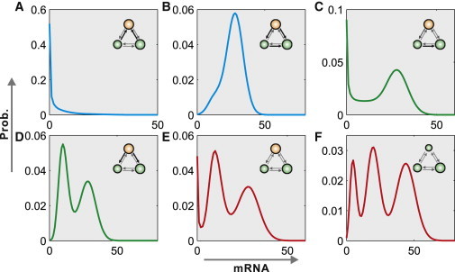
Numerical steady-state multimodal distributions of different modes in gene models with the same transition pattern between promoter activity states. The inactive state is denoted by orange whereas active states by green; thick arrows represent large transition rates whereas thin arrows represent small transition rates; large circles correspond to large transcription rates where small circles to small transcription rates. The two distributions indicated by the red imply that multiple exits of transcription are the essential source of generating multimodal distributions. The parameter values used in the computation are found in the Supporting Material. To see this figure in color, go online.

Mean waiting time distributions exhibit different characteristics albeit similar mRNA distributions

Experiments that reveal the dynamics of transcription initiation at promoters can reveal molecular mechanisms of transcription regulation (64). Several such experiments, where the synthesis of new mRNA molecules was visualized in live cells using single-molecule resolution technology, have been carried out in bacteria or eukaryotic cells (8,9,39), demonstrating that transcription occurs in a burst fashion. In these experiments, the spatial distribution of polymerases along a gene may bear the fingerprint of the time series of transcription initiation events, which is in turn determined by promoter dynamics. In response to experiments that probe transcription dynamics in single cells, in this study we consider how regulatory architecture modifies the probability distribution of mean waiting times between transcription initiation events. These times are experimentally testable. Here the goal is to provide experimental signatures predicted by theory that are capable of distinguishing between different mechanisms of transcriptional regulation.

First, we give the analytical results. Consider a gene model with the transition matrix among promoter activity states, denoted by $\mathbf{A=}\left(\begin{array}{cc}{\mathbf{A}}_{00}& {\mathbf{A}}_{10}\\ {\mathbf{A}}_{01}& {\mathbf{A}}_{11}\end{array}\right)$, where ${\mathbf{A}}_{00}$ describes the internal transitions between OFF states and the transitions from some ON states to OFF states; ${\mathbf{A}}_{10}$ and ${\mathbf{A}}_{01}$ describe transitions from ON to OFF states and from OFF to ON states, respectively; and ${\mathbf{A}}_{11}$ describes the internal transitions between ON states and the transitions from some OFF states to ON states. Then, the distribution functions for the mean ON and OFF times are computed according to the following formulae:

$$f_{off}\left(\tau \right)={\mathbf{u}}_L{\mathbf{A}}_{01}\exp \left({\mathbf{A}}_{00}\tau \right){\mathbf{A}}_{10}{\mathbf{u}}_L^T,f_{on}\left(\tau \right)={\mathbf{u}}_K{\mathbf{A}}_{10}\exp \left({\mathbf{A}}_{11}\tau \right){\mathbf{A}}_{01}{\mathbf{u}}_K^T$$ (2)

and, the mean waiting times at OFF and ON states are given by the following:

$$\langle {\tau }_{OFF}\rangle =\frac{1}{{\mathbf{u}}_L{\mathbf{A}}_{10}{\mathbf{u}}_L^T}{\mathbf{u}}_L{\mathbf{A}}_{01}{\left({\mathbf{A}}_{00}\right)}^{-2}{\mathbf{A}}_{10}{\mathbf{u}}_L^T,\langle {\tau }_{ON}\rangle =\frac{1}{{\mathbf{u}}_K{\mathbf{A}}_{01}{\mathbf{u}}_K^T}{\mathbf{u}}_K{\mathbf{A}}_{10}{\left({\mathbf{A}}_{11}\right)}^{-2}{\mathbf{A}}_{01}{\mathbf{u}}_K^T$$ (3)

where the row vectors ${\mathbf{u}}_L=\left(1,1,\cdots ,1\right)$ and ${\mathbf{u}}_K=\left(1,1,\cdots ,1\right)$ with $L$ and $K$ being the order of ${\mathbf{A}}_{00}$ and ${\mathbf{A}}_{11}$, respectively. See the Model and Method section for their derivation. The above formulae indicate that mean ON and OFF time distributions as well as mean ON and OFF times are easily computed as long as the transition matrix $\mathbf{A}$ is determined. For example, for a gene model where the promoter has two ON states and one OFF state that together constitute a loop, we have the following:

$$\langle {\tau }_{off}\rangle =\frac{1}{-a_{11}}\text{,}\langle {\tau }_{on}\rangle =\frac{1}{-a_{11}}\frac{c_2+c_3}{c_1}$$ (4)

where $c_i$ is the algebraic complement of the diagonal element $a_{ii}$ of the transition matrix $\mathbf{A}$ $\left(i=1,2,3\right)$.

Then, we perform numerical simulation. Consider two gene models with different PSs (see insets in Fig. 2 A and B) . We observe that two mRNA distributions exhibit the similar bimodal shape with two nontrivial peaks (the bimodality in Fig. 2 A is generated because of two distinct transcription exits whereas the one of two peaks in Fig. 2 B, which is closed to the y axis, is generated because of the cumulating effect of multiple inactive states and the other peak results from the transcription exit), but the mean ON and OFF times display different characteristics. Specifically, for the model in Fig. 2 A, the peak for the mean OFF time is close to zero whereas for the model in Fig. 2 B, the peak for the mean OFF time is away from zero (i.e., nontrivial peak); the mean ON time distributions exhibit different shapes for the time close to zero. Moreover, the time series of the ON states display different dynamical behaviors (compare the insets of Fig. 2 A and B).

Figure 2.

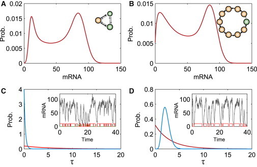
Two mRNA number distributions (A, B) look similar, but ON and OFF time distributions (C, D) exhibit different characteristics. In (C) and (D), the red lines correspond to ON whereas the blue lines to OFF. The insets show the time series of mRNAs and describe the time change of ON (red) and OFF states (green). The meaning of symbols in the inset of (A) and (B) is the same as in Fig. 1. The parameter values used in the computation are found in the Supporting Material. To see this figure in color, go online.

The above results indicate that on the one hand, the PS determines the mean ON and OFF times and their distributions; on the other hand, the characteristics of mean ON and OFF time distributions or those of the time series of ON and OFF states or both can provide the additional information on PS, thus enabling a remedy when the characteristics of mRNA distributions are insufficient to infer the PS.

Mean ON and OFF times together can characterize the transcriptional noise

For a gene model, the mRNA noise has two origins: one from the promoter fluctuations (called as the promoter noise) attributable to stochastic transitions among promoter activity states, and the other from stochastic synthesis and degradation of mRNA. The former is called the mRNA external noise whereas the latter the mRNA internal noise. The noise of the two kinds would together contribute to the generation of cell-to-cell variability.

For a multistate gene model, the mRNA internal noise is easy to describe since it can be characterized by the inverse of the mean mRNA number under our assumption. In contrast, describing the mRNA external noise is more difficult because of the complex PS. Therefore, we will focus on the promoter noise in the following.

Note that for the common ON-OFF model, the formula for computing the mRNA noise intensity, denoted by ${\eta }_m$, is the following:

$${\eta }_m^2=\frac{1}{\langle m\rangle }+\frac{{\langle {\tau }_{off}\rangle }^2}{\langle {\tau }_{on}\rangle +\langle {\tau }_{off}\rangle +\langle {\tau }_{on}\rangle \langle {\tau }_{off}\rangle }$$ (5)

where the first term on the right side of Eq. 5 represents the internal noise of mRNA from transcription, which is the inverse of the mRNA mean; the second term describes the promoter noise, denoted by ${\eta }_{promoter}^2$, which is a nonlinear function of mean ON and OFF times, denoted by $F\left(\langle {\tau }_{on}\rangle ,\langle {\tau }_{off}\rangle \right)$. In the Model and Method section, we show that for any gene model, the intensity of the noise in mRNA can be computed according to the following:

$${\eta }_m^2=\frac{1}{b_1}+\frac{2b_2-b_1^2}{b_1^2}$$ (6)

where $b_1$ and $b_2$ represent the first- and second-order binomial moments, respectively. Note that $b_1$ is the mRNA mean $\langle m\rangle$. Therefore, in analog to Eq. 5, it is reasonable to adopt the following formula to compute the intensity of the promoter noise:

$${\eta }_{promoter}^2=\frac{2b_2-b_1^2}{b_1^2}$$ (7)

According to the Model and Method section, this formula indicates that the promoter noise depends not only on transition matrix among promoter activity states but also on the transcription matrix since $b_1$ and $b_2$ depends on transition and transcription rates except in particular cases, e.g., all the transcription rates are precisely the same.

For example, consider the gene model studied in the previous subsection, i.e., the one where the promoter has two ON states and one OFF state. We can show the following:

$$b_1=\frac{\langle {\tau }_{off}\rangle }{\langle {\tau }_{on}\rangle +\langle {\tau }_{off}\rangle }\left({\mu }_1\frac{c_2}{c_1}+{\mu }_2\frac{c_3}{c_1}\right)$$ (8)

$$b_2=\frac{1}{2\det \left(\mathbf{I}-\mathbf{A}\right)\left(c_1+c_2+c_3\right)}\left[c_2{\mu }_1^2{A}_{22}^{\left(1\right)}+{\mu }_1{\mu }_2\left(c_2{A}_{23}^{\left(1\right)}+c_3{A}_{32}^{\left(1\right)}\right)+c_3{\mu }_2^2{A}_{33}^{\left(1\right)}\right]$$ (9)

where $A_{ij}^{\left(1\right)}$ are elements of the transposed matrix ${\left(\mathbf{I}-\mathbf{A}\right)}^T$, $i,j=2,3$. See the next section for their derivation. Therefore, ${\eta }_{promoter}^2$ depends in general on transcription rates ${\mu }_1$ and ${\mu }_2$ unless ${\mu }_1={\mu }_2$. Note that Eqs. 4, 8, and 9 are easily extended to the case that the promoter has one OFF and multiple ON states that together form a loop or one ON and multiple OFF states that together constitute a loop as well.

Next, we perform numerical analysis for the promoter noise. Fig. 3 plots the dependence of the promoter noise intensity $\left({\eta }^2\right)$ computed by Eq. 7 in combination with Eqs. 8 and 9 on the referred quantity $F\left(\langle {\tau }_{on}\rangle ,\langle {\tau }_{off}\rangle \right)$ with Eq. 4. In this figure, different symbols correspond to different PSs whereas the same symbols correspond to different transition patterns with the fixed promoter state number and the fixed transcription rates. More precisely, for a fixed PS and transcription rates, we have different dependences of ${\eta }^2$ on $F\left({\tau }_{ON},{\tau }_{OFF}\right)$ as the transition rates are randomly changed.

Figure 3.

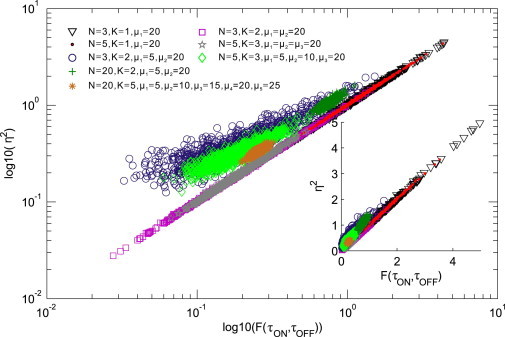
As an example of promoter structure, if all the transcription rates are precisely the same, then ${\log }_{10}\left({\eta }^2\right)$ vs. ${\log }_{10}F\left({\tau }_{ON},{\tau }_{OFF}\right)$ is located on a line and will deviate from the line otherwise. Here the abscissa represents the logarithm of the quantity $F\left({\tau }_{ON},{\tau }_{OFF}\right)$ computed according to Eq. 5, whereas the y axis represents the logarithm of the square of the promoter noise intensities computed by Eq. 7. Different symbols correspond to different promoter structures, whereas the same symbols correspond to different transition patterns with a fixed promoter state number and fixed transcription rates. The inset corresponds to the case without the logarithm. To see this figure in color, go online.

We observe that the differences among transcription rates have important influences on the deviation of the indicated symbols from the line with the slope equal to 1. Specifically, if all the promoter states are ON and all the transcription rates are precisely the same, then there is no promoter noise. In fact, in this case we can show that the corresponding mRNA number follows a Poisson distribution with the characteristic parameter being the common transcription rate, which is independent of the PS (see the Supporting Material). If a part of promoter states are ON and all the corresponding transcription rates are precisely the same, then the dependence of ${\eta }^2$ on $F\left({\tau }_{ON},{\tau }_{OFF}\right)$ is basically orientated on this slope, depending on transition rates regardless of the transition pattern among promoter activity states. This case implies that Eq. 7 can be used to quantify the promoter noise whose level is determined completely by the mean ON and OFF times. In other cases, we find that the larger the differences among transcription rates are because of, e.g., the regulation of TFs, the greater is the deviation of the indicated symbols from the line with the slope equal to 1, implying that the Eq. 7 cannot be used to approximate the promoter noise intensity. Such a nonlinear relationship can provide useful information on PS.

In other words, the promoter noise and also the mRNA noise depend in general on the transition pattern among the promoter activity states as well as the transcription exits; the mean ON and OFF times that are experimentally measurable can be used to characterize the promoter noise and the mRNA noise, thus providing signatures useful for inferring PS.

Model and Method

For the convenience of applications, in this section we consider a general gene model where the promoter has several ON and OFF states among which transitions may exist, and we give general formulae for computing steady-state mRNA distributions, mean waiting times, and waiting time distributions. These formulas are very useful and contain previous results obtained in simple gene models (e.g., the common ON-OFF model (14,17,19,22,56–58) and gene models of promoter-progression (25,26)) as their particular cases.

Model description

Assume that the promoter has $N$ states, $L$ states of which are active (denoted by ${\text{A}}_i$) and the other $K=N-L$ are inactive (denoted by $I_j$). Let matrices ${\mathbf{A}}_{11}$ and ${\mathbf{A}}_{00}$ describe transitions among the active states and among the inactive states, respectively. The matrix ${\mathbf{A}}_{10}$ describes how the active states transition to the inactive states, and similarly for matrix ${\mathbf{A}}_{01}$. These matrices, called as the transition matrices, together describe the PS partially. Denote by $m$, the number of mRNA molecules, and let $P_k\left(m\right)$ represent the distribution that mRNA has $m$ molecules at state-$k$ of the promoter and let $\mathbf{P}={\left(P_1,\cdots ,P_N\right)}^{\mathrm{T}}$ represent the column vector. Denote by ${\lambda }_{ij}$, the transition rate from state-$j$ to state-$i$ (${\lambda }_{ij}=0$ means that no transition occurs), the size of which may be regulated by TFs. Denote by $\mathbf{A}=\left({\lambda }_{ij}\right)$, the $N\times N$ transition matrix, which consist of four block matrices ${\mathbf{A}}_{11}$, ${\mathbf{A}}_{00}$, ${\mathbf{A}}_{10}$, and ${\mathbf{A}}_{01}$; and let $\mathbf{\Lambda }=\mathrm{diag}\left({\mu }_1,\cdots ,{\mu }_N\right)$ describe the exits of transcription (called transcription matrix) with ${\mu }_i$ representing the transcription rate of mRNA in state-$i$ (${\mu }_i=0$ means that no transcription takes place). Two matrices $\mathbf{A}$ and $\mathbf{\Lambda }$ together describe the PS completely. Then, the biochemical master equation describing mRNA dynamics takes the following form:

$$\frac{d\mathbf{P}\left(m;t\right)}{dt}=\mathbf{AP}\left(m;t\right)\mathbf{+\delta }\left(\mathbf{E}-\mathbf{I}\right)\left[m\mathbf{P}\left(m;t\right)\right]+\mathbf{\Lambda }\left({\mathbf{E}}^{-1}-\mathbf{I}\right)\left[\mathbf{P}\left(m;t\right)\right]$$ (10)

where $\mathbf{E}$ and ${\mathbf{E}}^{-1}$ are shift operators, and $\mathbf{I}$ is the identity operator. Clearly, the first term in Eq. 10 describes dynamics of the promoter with the transition matrix $\mathbf{A}$ that is actually an M-matrix (since the sum of every column elements is equal to zero); the second term describes the degradation dynamics of mRNA with the degradation matrix $\mathbf{\delta }$ that is a diagonal matrix (throughout this paper, we consider only the same degradation rate for simplicity, and denote it as $\delta$); and the third term describes the exits of transcription with the transcription matrix $\mathbf{\Lambda }$. We point out that the model in Eq. 10 includes all previously studied mRNA expression models as its particular cases.

Computation of mRNA distributions

To solve Eq. 10, we introduce probability-generating functions of the vector form $\mathbf{G}={\left(G_1,\cdots ,G_N\right)}^{\mathrm{T}}$ with every component $G_k\left(z;t\right)={\sum }_{m\ge 0}{z}^m{P}_k\left(m;t\right)$ for the distributions of the vector form $\mathbf{P}\left(m;t\right)$. Then, from Eq. 10, we can derive the following linear system of partial differential equations:

$$\frac{\partial }{\partial t}\mathbf{G}=\mathbf{AG}-s\frac{\partial }{\partial s}\mathbf{G}+s\mathbf{\Lambda G}$$ (11)

where $s=z-1$ is taken as a new variable, and all the system parameters are rescaled by $\delta$. Note that Eq. 11 is an equivalent version of the biochemical master equation in Eq. 10 because of the relationship between the probability distribution and the generating function. This equivalence can help us find solutions to Eq. 11. Now, we expand every generating function as $G_k\left(s\right)={\sum }_{n=0}^{\infty }{a}_n^{\left(k\right)}{s}^n$. Then, we can show the following:

$$a_k^{\left(i\right)}\left(t\right)=\sum _{m\ge k}\left(\begin{array}{c}m\\ k\end{array}\right)P_i\left(\mathit{m};t\right)$$ (12)

where $\left(\begin{array}{c}m\\ k\end{array}\right)$ represents the common binomial coefficient. Therefore, the fixed $i$,$a_k^{\left(i\right)}\left(t\right)$ are called as binomial moments (65,66) corresponding to the probability $P_i\left(\mathit{m};t\right)$. In particular, $b_k={\sum }_{i=1}^N{a}_k^{\left(i\right)}$ are the total binomial moments corresponding to the total probability $P={\sum }_{i=1}^N{P}_i$. Note that $b_0=1$ because of the conservative condition ${\sum }_{m=0}^{\infty }P\left(m\right)=1$. Denote ${\mathbf{a}}_n={\left(a_n^{\left(1\right)},a_n^{\left(2\right)},\cdots ,a_n^{\left(N\right)}\right)}^T$. Then, from Eq. 11 we attain the following:

$$\frac{d}{dt}{\mathbf{a}}_n=-\left(n\mathbf{I}-\mathbf{A}\right){\mathbf{a}}_n+\mathbf{\Lambda }{\mathbf{a}}_{n-1}$$ (13)

which is a linear ordinary differential equation that is easily solved. Once all $a_k^{\left(i\right)}\left(t\right)$ are given, then the distribution $P_i\left(\mathit{m};t\right)$ is computed according to the following:

$$P_i\left(m;t\right)=\sum _{k\ge m}{\left(-1\right)}^{k-m}\left(\begin{array}{c}k\\ m\end{array}\right)a_k^{\left(i\right)}\left(t\right)$$ (14)

In particular, we can give analytical results at steady state. In fact, if we denote the total steady-state generating function $G\left(s\right)={\sum }_{k=1}^N{G}_k\left(s\right)$ with $G\left(0\right)=1$ and Taylor expand $G\left(s\right)={\sum }_{n=0}^{\infty }{b}_n{s}^n$, then it is not difficult to show ${\mu }_1{G}_1\left(s\right)+\cdots +{\mu }_N{G}_N\left(s\right)=G^{\text{'}}\left(s\right)$ since $\mathbf{A}$ is an M-matrix. We find that $b_n$ takes the following form:

$$b_n=\frac{1}{n}{\sum }_{i=1}^N{\mu }_i{a}_{n-1}^{\left(i\right)}=\frac{1}{n}{\mathbf{u}}_N\mathbf{\Lambda }{\mathbf{a}}_{n-1}$$ (15)

which is useful for deriving analytical distributions, where ${\mathbf{u}}_N=\left(1,1,\cdots ,1\right)$ is a row vector and ${\mathbf{a}}_n={\left(a_n^{\left(1\right)},a_n^{\left(2\right)},\cdots ,a_n^{\left(N\right)}\right)}^T$ is a column vector. Substituting the expansions of $G_k\left(s\right)$ into Eq. 11 at steady state, we see that the vector ${\mathbf{a}}_n$ satisfies the following algebraic equations:

$$\left(n\mathbf{I}-\mathbf{A}\right){\mathbf{a}}_n=\mathbf{\Lambda }{\mathbf{a}}_{n-1},n=1,2,\cdots$$ (16)

where ${\mathbf{a}}_0$ can be analytically given (see the Supporting Material). When Eq. 16 is combined with Eq. 15, then $b_n$ can be formally expressed as the following:

$$b_n=\frac{1}{n!{\prod }_{k=1}^n\det \left(k\mathbf{I}-\mathbf{A}\right)}{\mathbf{u}}_N\prod _{k=n}^1\left[{\left(k\mathbf{I}-\mathbf{A}\right)}^{\ast }\mathbf{\Lambda }\right]{\mathbf{a}}_0,n=1,2,\cdots$$ (17)

where ${\left(k\mathbf{I}-\mathbf{A}\right)}^{\ast }$ and $\det \left(k\mathbf{I}-\mathbf{A}\right)$ are the adjacency matrix and the determinant of matrix $\left(k\mathbf{I}-\mathbf{A}\right)$, respectively; ${\mathbf{a}}_0$ is given in the Supporting Material. Such a formal expression of $b_n$ does not impose any condition on the transition matrix $\mathbf{A}$ and the transcription matrix $\mathbf{\Lambda }$.

Equation 17 indicates that Eq. 11 at steady state is solvable. Furthermore, Eq. 10 at steady state is also solvable. In some cases, the steady-state distributions can be expressed by confluent hypergeometric functions (67–70). Refer to the Supporting Material. In any case, $P\left(m\right)$ can be approximately computed up to a desired accuracy because $b_n\to 0$ as $n\to \infty$ (65). We point out that such a binomial moment method can be generalized to the stochastic analysis of any reaction networks. The details will be published elsewhere.

Computation of waiting time distributions and mean waiting times

Given a transition matrix $\mathbf{A}$ that is expressed as a block matrix of the form $\left(\begin{array}{cc}{\mathbf{A}}_{00}& {\mathbf{A}}_{10}\\ {\mathbf{A}}_{01}& {\mathbf{A}}_{11}\end{array}\right)$, where ${\mathbf{A}}_{00}$, ${\mathbf{A}}_{11}$, ${\mathbf{A}}_{10}$ and ${\mathbf{A}}_{01}$ are the $K\times K$, $L\times L$, $K\times L$ and $L\times K$ matrix, respectively, we derive the waiting-time distribution functions for ON and OFF states. Assume that the promoter states begin to transition from OFF (ON) to ON (OFF) at time $t=0$, and we define $Q_i^{\left(1\right)}\left(\tau \right)\left(i=1,\cdots ,L\right)$ and $Q_k^{\left(0\right)}\left(\tau \right)\left(k=1,\cdots ,K\right)$ as the subsequent “survival” probability that the promoter is still at the $i^{th}$ ON and at the $k^{th}$ OFF state at the time $t=\tau >0$, respectively. Then, the master equations for $Q_i^{\left(0\right)}\left(\tau \right)$ and $Q_i^{\left(1\right)}\left(\tau \right)$ take the following form:

$$\begin{array}{c}\frac{d{\mathbf{Q}}^{\left(0\right)}\left(\tau \right)}{d\tau }={\mathbf{A}}_{00}{\mathbf{Q}}^{\left(0\right)}\left(\tau \right)\\ \frac{d{\mathbf{Q}}^{\left(1\right)}\left(\tau \right)}{d\tau }={\mathbf{A}}_{11}{\mathbf{Q}}^{\left(1\right)}\left(\tau \right)\end{array}$$ (18)

respectively, where ${\mathbf{Q}}^{\left(0\right)}\left(\tau \right)={\left(Q_1^{\left(0\right)}\left(\tau \right),\cdots ,Q_K^{\left(0\right)}\left(\tau \right)\right)}^{\text{T}}$, ${\mathbf{Q}}^{\left(1\right)}\left(\tau \right)={\left(Q_1^{\left(1\right)}\left(\tau \right),\cdots ,Q_L^{\left(1\right)}\left(\tau \right)\right)}^{\text{T}}$. The solution to Eq. 18 can be expressed as the following:

$$\begin{array}{c}{\mathbf{Q}}^{\left(0\right)}\left(\tau \right)=\exp \left({\mathbf{A}}_{00}\tau \right){\mathbf{Q}}^{\left(0\right)}\left(0\right)\\ {\mathbf{Q}}^{\left(1\right)}\left(\tau \right)=\exp \left({\mathbf{A}}_{11}\tau \right){\mathbf{Q}}^{\left(1\right)}\left(0\right)\end{array}$$ (19)

Thus, for two given sets of initial survival probabilities $\left\{Q_1^{\left(0\right)}\left(0\right),\cdots ,Q_K^{\left(0\right)}\left(0\right)\right\}$ and $\left\{Q_1^{\left(1\right)}\left(0\right),\cdots ,Q_L^{\left(1\right)}\left(0\right)\right\}$, the distribution functions for the dwell times $\tau$ at the OFF and ON states are given by the following:

$$\begin{array}{c}{\tilde{f}}_{off}\left(\tau \right)={\mathbf{u}}_L{\mathbf{A}}_{01}{\mathbf{Q}}^{\left(0\right)}\left(\tau \right)={\mathbf{u}}_L{\mathbf{A}}_{01}\exp \left({\mathbf{A}}_{00}\tau \right){\mathbf{Q}}^{\left(0\right)}\left(0\right)\\ {\tilde{f}}_{on}\left(\tau \right)={\mathbf{u}}_K{\mathbf{A}}_{10}{\mathbf{Q}}^{\left(1\right)}\left(\tau \right)={\mathbf{u}}_K{\mathbf{A}}_{10}\exp \left({\mathbf{A}}_{11}\tau \right){\mathbf{Q}}^{\left(1\right)}\left(0\right)\end{array}$$ (20)

From Eq. 20, we can see that each of two distribution functions is in general a linear combination of exponential functions of the form $e^{{\lambda }_j\tau }$, so the result is an extension of that found in previous studies (71–73). Furthermore, the mean OFF and ON times can be computed by substituting ${\tilde{f}}_{off}\left(\tau \right),{\tilde{f}}_{on}\left(\tau \right)$ into the general expression $\langle \tau \rangle ={\int }_0^{\infty }\tau f\left(\tau \right)d\tau$, which attains the following:

$$\begin{array}{c}\langle {\tilde{\tau }}_{OFF}\rangle ={\int }_0^{\infty }\tau {\mathbf{u}}_L{\mathbf{A}}_{01}\exp \left({\mathbf{A}}_{00}\tau \right){\mathbf{Q}}^{\left(0\right)}\left(0\right)d\tau ={\mathbf{u}}_L{\mathbf{A}}_{01}{\left({\mathbf{A}}_{00}\right)}^{-2}{\mathbf{Q}}^{\left(0\right)}\left(0\right)\\ \langle {\tilde{\tau }}_{ON}\rangle ={\int }_0^{\infty }\tau {\mathbf{u}}_K{\mathbf{A}}_{10}\exp \left({\mathbf{A}}_{11}\tau \right){\mathbf{Q}}^{\left(1\right)}\left(0\right)d\tau ={\mathbf{u}}_K{\mathbf{A}}_{10}{\left({\mathbf{A}}_{11}\right)}^{-2}{\mathbf{Q}}^{\left(1\right)}\left(0\right)\end{array}$$ (21)

However, Eq. 21 is not the resulting mean waiting times at OFF and ON states since the initial survival probabilities ${\mathbf{Q}}^{\left(0\right)}\left(\tau \right)$ and ${\mathbf{Q}}^{\left(1\right)}\left(\tau \right)$ depend on the transition pattern among ON and OFF states. For a given PS, to obtain the total OFF and ON dwell times, we have to average $\langle {\tilde{\tau }}_{OFF}\rangle$ or $\langle {\tilde{\tau }}_{ON}\rangle$ over all such ON states that transition to OFF states or over all such OFF states that transition to ON states. For example, to compute the resulting $f_{on}\left(\tau \right)$, one should choose $Q_i^{\left(1j\right)}\left(0\right)=\left({\sum }_{l=1}^L{a}_{il}^{\left(0\to 1\right)}/{\sum }_{k=1}^K{\sum }_{l=1}^L{a}_{kl}^{\left(0\to 1\right)}\right){\delta }_{ij}\left(j,i=1,\cdots ,K\right)$ as the initial conditions, where ${\delta }_{ij}$ is the Kronecker delta; and for clarity and convenience, we let $a_{ik}^{\left(0\to 1\right)}$ represent the transition rate from the $k^{th}$ OFF state to the $i^{th}$ ON state (similarly, $a_{ik}^{\left(1\to 0\right)}$, $a_{ik}^{\left(0\to 0\right)}$, and $a_{ik}^{\left(1\to 1\right)}$). The resulting distribution functions for the mean ON and OFF times are computed according to the following:

$$\begin{array}{c}{f}_{off}\left(\tau \right)={\mathbf{u}}_L{\mathbf{A}}_{01}\exp \left({\mathbf{A}}_{00}\tau \right){\mathbf{A}}_{10}{\mathbf{u}}_L^T\\ f_{on}\left(\tau \right)={\mathbf{u}}_K{\mathbf{A}}_{10}\exp \left({\mathbf{A}}_{11}\tau \right){\mathbf{A}}_{01}{\mathbf{u}}_K^T\end{array}$$ (22)

whereas the resulting mean dwell times at OFF and ON states are given by the following:

$$\begin{array}{c}\langle {\tau }_{OFF}\rangle =\frac{1}{{\mathbf{u}}_L{\mathbf{A}}_{10}{\mathbf{u}}_L^T}{\mathbf{u}}_L{\mathbf{A}}_{01}{\left({\mathbf{A}}_{00}\right)}^{-2}{\mathbf{A}}_{10}{\mathbf{u}}_L^T\\ \langle {\tau }_{ON}\rangle =\frac{1}{{\mathbf{u}}_K{\mathbf{A}}_{01}{\mathbf{u}}_K^T}{\mathbf{u}}_K{\mathbf{A}}_{10}{\left({\mathbf{A}}_{11}\right)}^{-2}{\mathbf{A}}_{01}{\mathbf{u}}_K^T\end{array}$$ (23)

Conclusions and Discussions

Transcription is a complex biochemical process, involving recruitment of TFs and DNA polymerases, chromatin remodeling, and a sequence of transitions between activity states of the promoter. Previous studies have shown that transcription occur either as pulsatile bursts or as Poisson-like accumulations, but how promoter dynamics quantitatively and qualitatively affect transcriptional dynamics remains to be fully explored. In this study, we have analyzed gene models that corporate the complexity of PS, focusing on the effects of the multi-ON mechanism on transcriptional dynamics. We have shown that multiple exits of transcription are the essential source of generating multimodal mRNA distributions (Fig. 1). In addition, we have demonstrated that in the ($\log F$,${\eta }^2$) plane, the larger the differences among transcription rates are, the higher is the nonlinearity describing the dependence of the transcriptional noise on PS (Fig. 3). These qualitative characteristics that still hold in more complex gene models reveal the essential mechanism of how promoter dynamics affect transcriptional dynamics.

In a previous study (59), we demonstrated that slow transitions between promoter states that can lead to a bimodal distribution of the mRNA copy number as observed in the two-state promoter model can also result in a unimodal distribution when the number of promoter states is larger than two. In this study, we have shown that multiple exits of transcription can lead to multimodal mRNA distributions, but there are exceptions, e.g., when all the promoter states are ON with the same transcription rate, which result in a Poisson distribution independent of PS. A more careful investigation of this issue would clarify whether distributions from multistate promoters can be clearly distinguished from those produced by two-state ON/OFF promoters, and how many events would be needed to see the difference in the experimental data. If it were found that two-state and multistate promoters cannot be clearly distinguished by virtue of the distribution, it would call into the question of how seriously we should take the fitting parameters extracted from fitting experimental distributions of mRNA numbers. We would like to point out that our model cannot exhibit bistability in the deterministic case but can exhibit stochastic multimodality including bistability in the stochastic case according to the definition in a previous study (74).

For gene models with more complex PS, which would correspond to complicated mathematical forms expressed in the master equation, the first- and second-order moments of mRNA can be derived using the same simple method used to compute the moments in the two-state promoter model. In fact, the formulas for the moments apply to any other promoter model as well, regardless of the number of promoter states. In addition, the focus of the analysis in this study is on mRNA noise, but the mathematical approaches to compute mRNA statistics can be easily extended to compute protein distributions and their moments as well. For instance, for a promoter switching between two different states, in the limit when mRNA lifetime is much shorter than protein lifetime, the ratio of variance over mean for protein takes the form very similar to that for mRNA. At least in this limit, all of the conclusions about how complex promoter dynamics affect mRNA noise would be qualitatively true for protein noise. In other words, all the related extension and computation are easily carried out in the case that TFs do not temporally regulate transition rates among the promoter activity states (47). However, the regulation of TFs is often dynamic and noisy. In this case, what is the dependence relationship between transcriptional output and TFs (as inputs) or how the latter affects the former deserves further study since analytical results (e.g., analytical distributions as derived in this paper) are in general unavailable. If the gene promoter has only one ON and one OFF state (i.e., the common gene model), one can use the input-associated Signed Activation Time (iSAT) index introduced in another study (75), which concisely captures an intrinsic temporal property at either the ON or OFF state, to characterize the input-output relation including the transcriptional noise. In the case of complex PS (i.e., the promoter has multiple ON or OFF states or both), the iSAT index would be still effective in quantifying this relation but its definition seems to need modification. By analyzing this modified index, it is possible to reveal which of the multiple ON and OFF mechanisms is dominant in buffering the transcriptional noise. In particular, it is possible that there is a tradeoff between achieving good noise buffering in the ON versus the OFF states as shown in a previous study(75). The further study is under way.

Finally, as with any quantitative model, especially one attempting to describe processes within a living cell, it is important to understand the limitations of the chemical master equation description of transcription presented in this paper. Particular care has to be taken when using mathematical models in conjunction with experimental data to test specific hypotheses about biological mechanisms. Even for most informative models, there would be a discrepancy between the model predictions and experimental data. This offers the opportunity to discard incorrect assumptions about the mechanisms of interest. But to reach such strong conclusions, we must have some degree of certainty that the discrepancy between the model predictions and experimental outcomes is because of the deficiencies in our understanding of the underlying biological mechanism, and not because of spurious experimental effects that have nothing to do with the biological process of interest. This is a particularly challenging problem when using cell-to-cell or temporal variability of cellular outputs as the experimental signature of a biological process because there are typically multiple sources of this variability, and we are interested in the only one of them. For example, if the variability of the transcriptional output of a single cell is used as the experimental signature of promoter dynamics, then we must make sure that this is indeed the dominant source of the observed fluctuations.

References

- 1.Ozbudak E.M., Thattai M., van Oudenaarden A. Regulation of noise in the expression of a single gene. Nat. Genet. 2002;31:69–73. doi: 10.1038/ng869. [DOI] [PubMed] [Google Scholar]
- 2.Elowitz M.B., Levine A.J., Swain P.S. Stochastic gene expression in a single cell. Science. 2002;297:1183–1186. doi: 10.1126/science.1070919. [DOI] [PubMed] [Google Scholar]
- 3.Blake W.J., KAErn M., Collins J.J. Noise in eukaryotic gene expression. Nature. 2003;422:633–637. doi: 10.1038/nature01546. [DOI] [PubMed] [Google Scholar]
- 4.Raser J.M., O’Shea E.K. Control of stochasticity in eukaryotic gene expression. Science. 2004;304:1811–1814. doi: 10.1126/science.1098641. [DOI] [PMC free article] [PubMed] [Google Scholar]
- 5.Boettiger A.N., Levine M. Synchronous and stochastic patterns of gene activation in the Drosophila embryo. Science. 2009;325:471–473. doi: 10.1126/science.1173976. [DOI] [PMC free article] [PubMed] [Google Scholar]
- 6.Raj A., Rifkin S.A., van Oudenaarden A. Variability in gene expression underlies incomplete penetrance. Nature. 2010;463:913–918. doi: 10.1038/nature08781. [DOI] [PMC free article] [PubMed] [Google Scholar]
- 7.Eldar A., Elowitz M.B. Functional roles for noise in genetic circuits. Nature. 2010;467:167–173. doi: 10.1038/nature09326. [DOI] [PMC free article] [PubMed] [Google Scholar]
- 8.Golding I., Paulsson J., Cox E.C. Real-time kinetics of gene activity in individual bacteria. Cell. 2005;123:1025–1036. doi: 10.1016/j.cell.2005.09.031. [DOI] [PubMed] [Google Scholar]
- 9.Raj A., Peskin C.S., Tyagi S. Stochastic mRNA synthesis in mammalian cells. PLoS Biol. 2006;4:e309. doi: 10.1371/journal.pbio.0040309. [DOI] [PMC free article] [PubMed] [Google Scholar]
- 10.Suter D.M., Molina N., Naef F. Mammalian genes are transcribed with widely different bursting kinetics. Science. 2011;332:472–474. doi: 10.1126/science.1198817. [DOI] [PubMed] [Google Scholar]
- 11.Harper C.V., Finkenstädt B., White M.R. Dynamic analysis of stochastic transcription cycles. PLoS Biol. 2011;9:e1000607. doi: 10.1371/journal.pbio.1000607. [DOI] [PMC free article] [PubMed] [Google Scholar]
- 12.Spiller D.G., Wood C.D., White M.R. Measurement of single-cell dynamics. Nature. 2010;465:736–745. doi: 10.1038/nature09232. [DOI] [PubMed] [Google Scholar]
- 13.Berg O.G. A model for the statistical fluctuations of protein numbers in a microbial population. J. Theor. Biol. 1978;71:587–603. doi: 10.1016/0022-5193(78)90326-0. [DOI] [PubMed] [Google Scholar]
- 14.Peccoud J., Ycart B. Markovian modeling of gene product synthesis. Theor. Popul. Biol. 1995;48:222–234. [Google Scholar]
- 15.McAdams H.H., Arkin A. Stochastic mechanisms in gene expression. Proc. Natl. Acad. Sci. USA. 1997;94:814–819. doi: 10.1073/pnas.94.3.814. [DOI] [PMC free article] [PubMed] [Google Scholar]
- 16.Thattai M., van Oudenaarden A. Intrinsic noise in gene regulatory networks. Proc. Natl. Acad. Sci. USA. 2001;98:8614–8619. doi: 10.1073/pnas.151588598. [DOI] [PMC free article] [PubMed] [Google Scholar]
- 17.Kepler T.B., Elston T.C. Stochasticity in transcriptional regulation: origins, consequences, and mathematical representations. Biophys. J. 2001;81:3116–3136. doi: 10.1016/S0006-3495(01)75949-8. [DOI] [PMC free article] [PubMed] [Google Scholar]
- 18.Paulsson J. Summing up the noise in gene networks. Nature. 2004;427:415–418. doi: 10.1038/nature02257. [DOI] [PubMed] [Google Scholar]
- 19.Paulsson J. Models of stochastic gene expression. Phys. Life Rev. 2005;2:157–175. [Google Scholar]
- 20.Raser J.M., O’Shea E.K. Noise in gene expression: origins, consequences, and control. Science. 2005;309:2010–2013. doi: 10.1126/science.1105891. [DOI] [PMC free article] [PubMed] [Google Scholar]
- 21.Friedman N., Cai L., Xie X.S. Linking stochastic dynamics to population distribution: an analytical framework of gene expression. Phys. Rev. Lett. 2006;97:168302. doi: 10.1103/PhysRevLett.97.168302. [DOI] [PubMed] [Google Scholar]
- 22.Shahrezaei V., Swain P.S. Analytical distributions for stochastic gene expression. Proc. Natl. Acad. Sci. USA. 2008;105:17256–17261. doi: 10.1073/pnas.0803850105. [DOI] [PMC free article] [PubMed] [Google Scholar]
- 23.Pedraza J.M., Paulsson J. Effects of molecular memory and bursting on fluctuations in gene expression. Science. 2008;319:339–343. doi: 10.1126/science.1144331. [DOI] [PubMed] [Google Scholar]
- 24.Sánchez A., Kondev J. Transcriptional control of noise in gene expression. Proc. Natl. Acad. Sci. USA. 2008;105:5081–5086. doi: 10.1073/pnas.0707904105. [DOI] [PMC free article] [PubMed] [Google Scholar]
- 25.Sánchez A., Garcia H.G., Kondev J. Effect of promoter architecture on the cell-to-cell variability in gene expression. PLOS Comput. Biol. 2011;7:e1001100. doi: 10.1371/journal.pcbi.1001100. [DOI] [PMC free article] [PubMed] [Google Scholar]
- 26.Sánchez A., Choubey S., Kondev J. Stochastic models of transcription: From single molecules to single cells. Methods. 2013;62:13–25. doi: 10.1016/j.ymeth.2013.03.026. [DOI] [PubMed] [Google Scholar]
- 27.Jia T., Kulkarni R.V. Intrinsic noise in stochastic models of gene expression with molecular memory and bursting. Phys. Rev. Lett. 2011;106:058102. doi: 10.1103/PhysRevLett.106.058102. [DOI] [PubMed] [Google Scholar]
- 28.Dobrzynski M., Bruggeman F.J. Elongation dynamics shape bursty transcription and translation. Proc. Natl. Acad. Sci. USA. 2009;106:2583–2588. doi: 10.1073/pnas.0803507106. [DOI] [PMC free article] [PubMed] [Google Scholar]
- 29.Rinott R., Jaimovich A., Friedman N. Exploring transcription regulation through cell-to-cell variability. Proc. Natl. Acad. Sci. USA. 2011;108:6329–6334. doi: 10.1073/pnas.1013148108. [DOI] [PMC free article] [PubMed] [Google Scholar]
- 30.Huh D., Paulsson J. Non-genetic heterogeneity from stochastic partitioning at cell division. Nat. Genet. 2011;43:95–100. doi: 10.1038/ng.729. [DOI] [PMC free article] [PubMed] [Google Scholar]
- 31.Hager G.L., McNally J.G., Misteli T. Transcription dynamics. Mol. Cell. 2009;35:741–753. doi: 10.1016/j.molcel.2009.09.005. [DOI] [PMC free article] [PubMed] [Google Scholar]
- 32.Vilar J.M.G., Saiz L. CplexA: a Mathematica package to study macromolecular-assembly control of gene expression. Bioinformatics. 2010;26:2060–2061. doi: 10.1093/bioinformatics/btq328. [DOI] [PubMed] [Google Scholar]
- 33.Hornung G., Bar-Ziv R., Barkai N. Noise-mean relationship in mutated promoters. Genome Res. 2012;22:2409–2417. doi: 10.1101/gr.139378.112. [DOI] [PMC free article] [PubMed] [Google Scholar]
- 34.Halme A., Bumgarner S., Fink G.R. Genetic and epigenetic regulation of the FLO gene family generates cell-surface variation in yeast. Cell. 2004;116:405–415. doi: 10.1016/s0092-8674(04)00118-7. [DOI] [PubMed] [Google Scholar]
- 35.Octavio L.M., Gedeon K., Maheshri N. Epigenetic and conventional regulation is distributed among activators of FLO11 allowing tuning of population-level heterogeneity in its expression. PLoS Genet. 2009;5:e1000673. doi: 10.1371/journal.pgen.1000673. [DOI] [PMC free article] [PubMed] [Google Scholar]
- 36.Weinberger L., Voichek Y., Barkai N. Expression noise and acetylation profiles distinguish HDAC functions. Mol. Cell. 2012;47:193–202. doi: 10.1016/j.molcel.2012.05.008. [DOI] [PMC free article] [PubMed] [Google Scholar]
- 37.Stavreva D.A., Varticovski L., Hager G.L. Complex dynamics of transcription regulation. Biochim. Biophys. Acta. 2012;1819:657–666. doi: 10.1016/j.bbagrm.2012.03.004. [DOI] [PMC free article] [PubMed] [Google Scholar]
- 38.Sánchez A., Choubey S., Kondev J. Regulation of noise in gene expression. Annu. Rev. Biophys. 2013;42:469–491. doi: 10.1146/annurev-biophys-083012-130401. [DOI] [PubMed] [Google Scholar]
- 39.Chubb J.R., Trcek T., Singer R.H. Transcriptional pulsing of a developmental gene. Curr. Biol. 2006;16:1018–1025. doi: 10.1016/j.cub.2006.03.092. [DOI] [PMC free article] [PubMed] [Google Scholar]
- 40.Chubb J.R., Liverpool T.B. Bursts and pulses: insights from single cell studies into transcriptional mechanisms. Curr. Opin. Genet. Dev. 2010;20:478–484. doi: 10.1016/j.gde.2010.06.009. [DOI] [PubMed] [Google Scholar]
- 41.Boeger H., Griesenbeck J., Kornberg R.D. Nucleosome retention and the stochastic nature of promoter chromatin remodeling for transcription. Cell. 2008;133:716–726. doi: 10.1016/j.cell.2008.02.051. [DOI] [PMC free article] [PubMed] [Google Scholar]
- 42.Larson D.R. What do expression dynamics tell us about the mechanism of transcription? Curr. Opin. Genet. Dev. 2011;21:591–599. doi: 10.1016/j.gde.2011.07.010. [DOI] [PMC free article] [PubMed] [Google Scholar]
- 43.Mao C., Brown C.R., Boeger H. Quantitative analysis of the transcription control mechanism. Mol. Syst. Biol. 2010;6:431. doi: 10.1038/msb.2010.83. [DOI] [PMC free article] [PubMed] [Google Scholar]
- 44.Mariani L., Schulz E.G., Höfer T. Short-term memory in gene induction reveals the regulatory principle behind stochastic IL-4 expression. Mol. Syst. Biol. 2010;6:359. doi: 10.1038/msb.2010.13. [DOI] [PMC free article] [PubMed] [Google Scholar]
- 45.Miller-Jensen K., Dey S.S., Arkin A.P. Varying virulence: epigenetic control of expression noise and disease processes. Trends Biotechnol. 2011;29:517–525. doi: 10.1016/j.tibtech.2011.05.004. [DOI] [PubMed] [Google Scholar]
- 46.Gama-Castro S., Salgado H., Collado-Vides J. RegulonDB version 7.0: transcriptional regulation of Escherichia coli K-12 integrated within genetic sensory response units (Gensor Units) Nucleic Acids Res. 2011;39(Suppl.):D98–D105. doi: 10.1093/nar/gkq1110. [DOI] [PMC free article] [PubMed] [Google Scholar]
- 47.Blake W.J., Balázsi G., Collins J.J. Phenotypic consequences of promoter-mediated transcriptional noise. Mol. Cell. 2006;24:853–865. doi: 10.1016/j.molcel.2006.11.003. [DOI] [PubMed] [Google Scholar]
- 48.To T.-L., Maheshri N. Noise can induce bimodality in positive transcriptional feedback loops without bistability. Science. 2010;327:1142–1145. doi: 10.1126/science.1178962. [DOI] [PubMed] [Google Scholar]
- 49.Bintu L., Buchler N.E., Phillips R. Transcriptional regulation by the numbers: models. Curr. Opin. Genet. Dev. 2005;15:116–124. doi: 10.1016/j.gde.2005.02.007. [DOI] [PMC free article] [PubMed] [Google Scholar]
- 50.Bintu L., Buchler N.E., Phillips R. Transcriptional regulation by the numbers: applications. Curr. Opin. Genet. Dev. 2005;15:125–135. doi: 10.1016/j.gde.2005.02.006. [DOI] [PMC free article] [PubMed] [Google Scholar]
- 51.Coulon A., Gandrillon O., Beslon G. On the spontaneous stochastic dynamics of a single gene: complexity of the molecular interplay at the promoter. BMC Syst. Biol. 2010;4:2. doi: 10.1186/1752-0509-4-2. [DOI] [PMC free article] [PubMed] [Google Scholar]
- 52.Simpson M.L., Cox C.D., Sayler G.S. Frequency domain chemical Langevin analysis of stochasticity in gene transcriptional regulation. J. Theor. Biol. 2004;229:383–394. doi: 10.1016/j.jtbi.2004.04.017. [DOI] [PubMed] [Google Scholar]
- 53.Höfer T., Rasch M.J. On the kinetic design of transcription. Genome Inform. 2005;16:73–82. [PubMed] [Google Scholar]
- 54.Carey L.B., van Dijk D., Segal E. Promoter sequence determines the relationship between expression level and noise. PLoS Biol. 2013;11:e1001528. doi: 10.1371/journal.pbio.1001528. [DOI] [PMC free article] [PubMed] [Google Scholar]
- 55.Brown C.R., Mao C., Boeger H. Linking stochastic fluctuations in chromatin structure and gene expression. PLoS Biol. 2013;11:e1001621. doi: 10.1371/journal.pbio.1001621. [DOI] [PMC free article] [PubMed] [Google Scholar]
- 56.Karmakar R., Bose I. Graded and binary responses in stochastic gene expression. Phys. Biol. 2004;1:197–204. doi: 10.1088/1478-3967/1/4/001. [DOI] [PubMed] [Google Scholar]
- 57.Iyer-Biswas S., Hayot F., Jayaprakash C. Stochasticity of gene products from transcriptional pulsing. Phys. Rev. E Stat. Nonlin. Soft Matter Phys. 2009;79:031911. doi: 10.1103/PhysRevE.79.031911. [DOI] [PubMed] [Google Scholar]
- 58.Mugler A., Walczak A.M., Wiggins C.H. Spectral solutions to stochastic models of gene expression with bursts and regulation. Phys. Rev. E Stat. Nonlin. Soft Matter Phys. 2009;80:041921. doi: 10.1103/PhysRevE.80.041921. [DOI] [PMC free article] [PubMed] [Google Scholar]
- 59.Zhang J., Chen L., Zhou T. Analytical distribution and tunability of noise in a model of promoter progress. Biophys. J. 2012;102:1247–1257. doi: 10.1016/j.bpj.2012.02.001. [DOI] [PMC free article] [PubMed] [Google Scholar]
- 60.Zhou T., Zhang J. Analytical results for a multistate gene model. SIAM J. Appl. Math. 2012;72:789–818. [Google Scholar]
- 61.Fraser D., Kaern M. A chance at survival: gene expression noise and phenotypic diversification strategies. Mol. Microbiol. 2009;71:1333–1340. doi: 10.1111/j.1365-2958.2009.06605.x. [DOI] [PubMed] [Google Scholar]
- 62.Acar M., Mettetal J.T., van Oudenaarden A. Stochastic switching as a survival strategy in fluctuating environments. Nat. Genet. 2008;40:471–475. doi: 10.1038/ng.110. [DOI] [PubMed] [Google Scholar]
- 63.Gillespie D.T. Exact stochastic simulation of coupled chemical reactions. J. Phys. Chem. 1977;81:2340–2361. [Google Scholar]
- 64.Friedman L.J., Gelles J. Mechanism of transcription initiation at an activator-dependent promoter defined by single-molecule observation. Cell. 2012;148:679–689. doi: 10.1016/j.cell.2012.01.018. [DOI] [PMC free article] [PubMed] [Google Scholar]
- 65.Takacs L. A moment problem. J. Austral. Math. Soc. 1965;5:487–490. [Google Scholar]
- 66.Zhang J., Nie Q., Zhou T. An effective method for computing the noise in biochemical networks. J. Chem. Phys. 2013;138:084106. doi: 10.1063/1.4792444. [DOI] [PMC free article] [PubMed] [Google Scholar]
- 67.Slater L.J. Cambridge University Press; Cambridge, UK: 1960. Confluent Hypergeometric Functions. [Google Scholar]
- 68.Okubo K. Connection problems for systems of linear differential equations. Lect. Notes in Math. 1971;243:238–248. [Google Scholar]
- 69.Schäfke R. Confluence of several regular singular points into an irregular singular point. J. Dyn. Contr. Syst. 1998;4:401–424. [Google Scholar]
- 70.Balser W., Röscheisen C. Solving the hypergeometric system of Okubo type in terms of a certain generalized hypergeometric function. J. Differ. Equ. 2009;247:2485–2494. [Google Scholar]
- 71.Tu Y. The nonequilibrium mechanism for ultrasensitivity in a biological switch: sensing by Maxwell’s demons. Proc. Natl. Acad. Sci. USA. 2008;105:11737–11741. doi: 10.1073/pnas.0804641105. [DOI] [PMC free article] [PubMed] [Google Scholar]
- 72.Li G., Qian H. Kinetic timing: a novel mechanism that improves the accuracy of GTPase timers in endosome fusion and other biological processes. Traffic. 2002;3:249–255. doi: 10.1034/j.1600-0854.2002.030402.x. [DOI] [PubMed] [Google Scholar]
- 73.Qian H. Phosphorylation energy hypothesis: open chemical systems and their biological functions. Annu. Rev. Phys. Chem. 2007;58:113–142. doi: 10.1146/annurev.physchem.58.032806.104550. [DOI] [PubMed] [Google Scholar]
- 74.Bishop L.M., Qian H. Stochastic bistability and bifurcation in a mesoscopic signaling system with autocatalytic kinase. Biophys. J. 2010;98:1–11. doi: 10.1016/j.bpj.2009.09.055. [DOI] [PMC free article] [PubMed] [Google Scholar]
- 75.Chen M., Wang L., Nie Q. Noise attenuation in the ON and OFF states of biological switches. ACS Synth Biol. 2013;2:587–593. doi: 10.1021/sb400044g. [DOI] [PMC free article] [PubMed] [Google Scholar]
Associated Data
This section collects any data citations, data availability statements, or supplementary materials included in this article.