The Movable Type Method Applied to Protein-Ligand Binding

Abstract

Accurately computing the free energy for biological processes like protein folding or protein-ligand association remains a challenging problem. Both describing the complex intermolecular forces involved and sampling the requisite configuration space make understanding these processes innately difficult. Herein, we address the sampling problem using a novel methodology we term “movable type”. Conceptually it can be understood by analogy with the evolution of printing and, hence, the name movable type. For example, a common approach to the study of protein-ligand complexation involves taking a database of intact drug-like molecules and exhaustively docking them into a binding pocket. This is reminiscent of early woodblock printing where each page had to be laboriously created prior to printing a book. However, printing evolved to an approach where a database of symbols (letters, numerals, etc.) was created and then assembled using a movable type system, which allowed for the creation of all possible combinations of symbols on a given page, thereby, revolutionizing the dissemination of knowledge. Our movable type (MT) method involves the identification of all atom pairs seen in protein-ligand complexes and then creating two databases: one with their associated pairwise distant dependent energies and another associated with the probability of how these pairs can combine in terms of bonds, angles, dihedrals and non-bonded interactions. Combining these two databases coupled with the principles of statistical mechanics allows us to accurately estimate binding free energies as well as the pose of a ligand in a receptor. This method, by its mathematical construction, samples all of configuration space of a selected region (the protein active site here) in one shot without resorting to brute force sampling schemes involving Monte Carlo, genetic algorithms or molecular dynamics simulations making the methodology extremely efficient. Importantly, this method explores the free energy surface eliminating the need to estimate the enthalpy and entropy components individually. Finally, low free energy structures can be obtained via a free energy minimization procedure yielding all low free energy poses on a given free energy surface. Besides revolutionizing the protein-ligand docking and scoring problem this approach can be utilized in a wide range of applications in computational biology which involve the computation of free energies for systems with extensive phase spaces including protein folding, protein-protein docking and protein design.

Introduction

Sampling the configuration space of complex biomolecules is a major hurdle impeding our ability to advance the understanding of a diverse range of processes including protein folding and the accurate prediction of ligand binding to a biological receptor.^1–10 Major advances have been made in computer hardware, which has allowed molecular dynamics (MD) simulations to reach the millisecond barrier, but this method is brute force in nature and requires highly sophisticated hardware and software.^2,10,11–14 Moreover, a major hurdle in the modeling of biological systems is associated with how the inter and intra-molecular energies are modeled. Modern force fields are highly evolved, but still need to be further refined to reach chemical accuracy in many applications.^9,14,15–17

Predicting how a ligand (drug) binds its receptor and predicting its associated binding affinity is a highly challenging problem, which if solved, would singularly advance modern structure-based drug design.^8,15,17–31 This approach has largely employed so-called end-point methods that dock (place) a candidate molecule into a receptor and compute the binding free energy using a range of physics-based or empirical “scoring” functions. From an analysis of the error propagation properties in the statistical mechanics based prediction of protein-ligand binding affinities it was shown that the end-point class of approaches maximizes energy function uncertainties.^32–34 This can be alleviated through the use of sampling approaches including MD methods or methods that exhaustively sample the configuration space associated with protein-ligand binding.^{1–3,5–7,9,11–14} These methods have shown that they can be successful, but are brute force in nature, which lead us to consider ways in which we can use ideas more akin to the endpoint methods, but incorporating sampling at the same time. The concept being that this approach would give us the best of both worlds, while mitigating the effects of energy function deficiencies.

Using MD or exhaustive sampling procedures to evaluate protein-ligand binding is conceptually similar to woodblock printing technology where all the words (molecules) are carefully placed on a board (receptor site) and the whole book can be printed (binding free energy determined). While a more advanced printing technology, movable type printing, (which was invented in China in the 11th century and introduced by Gutenberg into the alphabetic language system) uses a “database” of letters that is pre-constructed and then the printing of any word involves a database search followed by the appropriate combination from the movable type system. Using a typical pairwise potential the molecular energy of a system can be decomposed into atom pairwise interaction energies including bond, angle, torsion, and long-range non-covalent forces (van der Waals and electrostatic forces), which by analogy to the MT systems is our database of “letters”. Each interaction has a different intensity and probability of occurrence along an atom pairwise coordinate axis. Herein, we develop the mathematics necessary to bring end-point methods up to the “movable type printing level”, via building a database of energy intensities and probabilities for all atom type pair interactions found in protein-ligand complexes. Using this information we then demonstrate that the MT approach enhances our ability to predict protein-ligand binding free energies and also allows us to extract the associated low energy poses all at a fraction of the cost associated with “brute” force sampling methods. Moreover, the docking and scoring problem is an example of a broad class of problems in computational biology that involve both the computation of the free energy and structure of a biological system, which includes challenges like the prediction of protein folds, protein-protein interactions and protein design all of which the MT method can address.

Methodology

The Movable Type Method Applied to Protein-Ligand Binding

A thermodynamic cycle modeling the binding free energy ΔG_b^s in solution (shown in Figure 1) is typically employed in end-point methods:

$$\mathrm{\Delta }{G}_b^s=\mathrm{\Delta }{G}_b^g+\mathrm{\Delta }{G}_{\mathit{solv}}^{PL}-\mathrm{\Delta }{G}_{\mathit{solv}}^L-\mathrm{\Delta }{G}_{\mathit{solv}}^P$$ (1)

where P and L indicate the protein and ligand, s and g represent the behavior in solution and the gas-phase, respectively, ΔG_solv is the solvation free energy, and ΔG_b is the binding free energy in gas (g) and solution (s), respectively.

Figure 1.

The thermodynamic cycle used to formulate the free energy of protein-ligand binding in solution.

Using $\mathrm{\Delta }\mathrm{\Delta }{G}_{\mathit{solv}}=\mathrm{\Delta }{G}_{\mathit{solv}}^{PL}-\mathrm{\Delta }{G}_{\mathit{solv}}^L-\mathrm{\Delta }{G}_{\mathit{solv}}^P$, Equation 1 becomes:

$$\mathrm{\Delta }{G}_b^s=\mathrm{\Delta }{G}_b^g-\mathrm{\Delta }\mathrm{\Delta }{G}_{\mathit{solv}}$$ (2)

The binding free energy in solution is now separated into two terms: The binding free energy in the gas-phase and the change in the solvation free energy during the complexation process. At this point we introduce the moveable type algorithm to model both terms each with its own design.

The binding free energy in the gas-phase is the most important term to evaluate in order to predict the protein-ligand binding affinity because it contains all interactions between the protein and ligand. When approximated as the Helmholtz free energy (NVT), the Gibbs (we use the canonical ensemble throughout, but will predominantly use the ΔG notation) binding free energy in the gas-phase can be generated using the ratio of the partition functions describing the protein-ligand complex, the protein, and the ligand.

$$\mathrm{\Delta }{G}_b^g\approx \mathrm{\Delta }{A}_b^g=-\mathit{RT}ln\left[\frac{Z_{PL}}{Z_P{Z}_L}\right]=-\mathit{RT}ln\left[\frac{\int e^{-\beta E_{PL}(r)}dr}{\int e^{-\beta E_P(r)}dr\int e^{-\beta E_L(r)}dr}\right]$$ (3)

where Z represents the canonical ensemble partition function, and β is the reciprocal of the thermodynamic temperature k_BT. Partition functions are integrals over all possible coordinates of the protein-ligand complex, the protein, and the ligand. Equation 3 can be manipulated into the following form:

$$\mathrm{\Delta }{G}_b^g=-\mathit{RT}ln\left[\frac{F_{PL}\langle e^{-\beta E_{PL}(r)}\rangle }{F_P\langle e^{-\beta E_P(r)}\rangle F_L\langle e^{-\beta E_L(r)}\rangle }\right]$$ (4)

where the partition functions are expressed as the Boltzmann-weighted average of the pose energies (shown in brackets) multiplied the volume of configuration space available to each state, shown as F in Equation 4. F_PL is approximated as the product of the external degrees of freedom (DoFs) of the bound protein and ligand (including the rotational and translational DoFs), and the internal DoFs of the bound protein and ligand (including the relative-positional and vibrational DoFs), given as:

$$F_{PL}=F_{\mathit{boundP}}^{\mathit{external}}{F}_{\mathit{boundL}}^{\mathit{external}}{F}_{\mathit{boundP}}^{\mathit{internal}}{F}_{\mathit{boundL}}^{\mathit{internal}}$$ (5)

Similarly, the DoFs of the free protein and ligand molecules are also separated into the external and internal components. Internal DoFs are identical for bound and free protein/ligand structures and the bound and free proteins are also assumed to share the same internal and external DoFs. Only the external DoFs of the ligand are differentiated between the bound and free systems. The rotational DoF of a free ligand is 8π² on a normalized unit sphere. However, because of the inaccessible volume present in protein-ligand systems, the rotational DoFs of bound ligands are designated as aπ² with a to-be-determined average volume factor a less than 8. The translational DoFs are treated as a constant C, which is assumed to be identical for all free ligands, while the translational DoF for bound ligands is the volume of the binding pocket V_pocket in which the ligands’ center of mass can translate. Thereby, in the protein-ligand binding process, changes in the DoFs can be modeled as a constant with respect to the different volumes of the binding pockets. Applying these approximations we obtain:

$$\frac{F_{PL}}{F_P{F}_L}=\frac{F_{\mathit{boundP}}^{\mathit{external}}{F}_{\mathit{boundP}}^{\mathit{external}}{F}_{\mathit{boundP}}^{\mathit{internal}}{F}_{\mathit{boundL}}^{\mathit{internal}}}{F_{\mathit{freeP}}^{\mathit{external}}{F}_{\mathit{freeP}}^{\mathit{internal}}\times F_{\mathit{freeL}}^{\mathit{external}}{F}_{\mathit{freeL}}^{\mathit{internal}}}=\frac{F_{\mathit{boundL}}^{\mathit{external}}}{F_{\mathit{freeL}}^{\mathit{external}}}=\frac{a{\pi }^2{V}_{\text{pocket}}}{8{\pi }^{2}C}=\frac{{aV}_{\text{pocket}}}{8C}$$ (6)

The gas-phase protein-ligand binding free energy can then be further manipulated into the following form:

$$\mathrm{\Delta }{G}_b^g=-\mathit{RT}ln\left[\frac{{aV}_{\text{pocket}}\langle e^{-\beta E_{PL}(r)}\rangle }{8C\langle e^{-\beta E_P(r)}\rangle \langle e^{-\beta E_L(r)}\rangle }\right]$$ (7)

Again using the Helmholtz free energy approximation (Equation 3), the solvation free energy can be correlated to the partition function of the solute (protein, ligand or protein-ligand complex) and solute-solvent bulk interactions. In this way, the solvation free energy, using $\mathrm{\Delta }{G}_{\mathit{solv}}^L$ as an example, is modeled as in Equation 8, and the DoFs are approximated as being the same for the solute and the solute-solvent bulk terms.

$$\mathrm{\Delta }{G}_{\mathit{solv}}^L\approx \mathrm{\Delta }{A}_{\mathit{solv}}^L=-\mathit{RT}ln\left[\frac{Z_{LS}}{Z_L}\right]=-\mathit{RT}ln\left[\frac{\int e^{-\beta E_{LS}(r)}dr}{\int e^{-\beta E_L(r)}dr}\right]=-\mathit{RT}ln\left[\frac{\langle e^{-\beta E_{LS}(r)}\rangle }{\langle e^{-\beta E_L(r)}\rangle }\right]$$ (8)

Finally, the remaining solvation terms given in Equation 1 ( $\mathrm{\Delta }{G}_{\mathit{solv}}^P$ and $\mathrm{\Delta }{G}_{\mathit{solv}}^P$) can be modeled in an analogous manner yielding the change in the solvation free energy as ligand binding occurs which then can be used to evaluate the overall free energy of ligand binding in aqueous solution.

Construction of the “Movable Type” System: Atom Pairwise Interaction Energy and Probability Databases

With pose energies sampled over all possible DoFs for the bound and free protein/ligand system, the gas-phase protein-ligand binding free energy can be generated using molecular dynamics, Monte Carlo, genetic algorithms, etc. by sampling over a large number of poses of the protein, ligand and protein-ligand complex. Using the canonical ensemble the Helmholtz free energy can be obtained as the arithmetic mean (sum of the energies of all ligand poses divided by the total number of all poses along with an estimate of integration volume) of Boltzmann factors:

$$G\approx A=-\mathit{RT}ln[Z]=-\mathit{RT}ln\left[\langle e^{-\beta E}\rangle \right]=-\mathit{RT}ln\left[\frac{{\displaystyle \sum _i}{e}^{-\beta E_i}}{N}\right]$$ (9)

However, the problem of pose-based energy sampling lies in the fact that pose selection and sample size significantly affect the final result, not to mention that calculating many unique poses is very time-consuming. Different ligand poses have different energy preferences for the binding site, which leads to a range of binding probabilities. When calculating the averaged partition functions in Equation 7, one can assign probabilities (Q) as weights to different Boltzmann factors in order to differentiate the binding pocket preferences against ligand poses, rather than just simply using an arithmetic mean of all Boltzmann factors.

$$Q_i=\frac{e^{-\beta E_i}}{{\displaystyle \sum _i}{e}^{-\beta E_i}}$$ (10)

$$G\approx A=-\mathit{RT}ln[Z]=-\mathit{RT}ln\left[\langle e^{-\beta E}\rangle \right]=-\mathit{RT}ln\left[\sum _i{Q}_i{e}^{-\beta E_i}\right]$$ (11)

The challenge in deriving the canonical partition function (as the denominator in Equation 10) for a protein-ligand system is that it is difficult to include all relevant ligand pose energies within the binding pocket using brute force sampling schemes. However, the task becomes much easier when a protein-ligand system is reduced to the atom-pair level. In this way the “pose” sampling problem can then can be cast as a 1-D rather than a 3-D problem by deriving the canonical partition function as a sum of the Boltzmann factor products of all atom pairwise energies included in the system over all atom pairwise separation distance ranges.

$$\begin{array}{l}Z=\sum _i^{\text{All}\text{Poses}}{Q}_i{e}^{-\beta E_i}\\ =\sum _p^{\text{All}\text{Combinations}}\prod _q^{\text{All}\text{atom}\text{pairs}}{Q}_{pq}{e}^{-\beta E_{pq}}\\ =\sum _{\alpha }^{\text{Bond}\text{Distance}\text{Range}}\prod _a^{\text{No}.\text{of}\text{Bonds}}{Q}_{a\alpha }{e}^{-\beta E_{a\alpha }}\times \sum _{\beta }^{\text{Angle}\text{Distance}\text{Range}}\prod _b^{\text{No}.\text{of}\text{Angles}}{Q}_{b\beta }{e}^{-\beta E_{b\beta }}\\ \times \sum _{\gamma }^{\text{Torsion}\text{Distance}\text{Range}}\prod _c^{\text{No}.\text{of}\text{Torsions}}{Q}_{c\gamma }{e}^{-\beta E_{c\gamma }}\times \sum _{\delta }^{\mathit{vdw}-\mathit{elec}\text{Distance}\text{Range}}\prod _d^{\text{No}.\text{of}\mathit{vdw}-\mathit{elec}\text{interactions}}{Q}_{d\delta }{e}^{-\beta E_{d\delta }}\end{array}$$ (12)

The canonical partition function can be derived following Equation 12, where the index “i” refers to each ligand pose (microstate) in a “traditional” brute force sampling scheme. When the protein-ligand system is broken down to the atom-pair level, “q” indicates all atom pairs in the molecular system, and “p” indicates each possible combination of all atom pairs each of which is at a pre-chosen distance. a, b, c and d refer to each atom pair as a bond, angle, torsion or long-range (van der Waals or electrostatic) interaction in the canonical system, respectively, and α, β, γ and δ refers to each sampled separation distance between the corresponding atom pair. Probabilities of all the atom pairwise distributions on the right hand side of Equation 12 are normalized as ( ${\displaystyle \sum _i}{Q}_i={\displaystyle \sum _i}\frac{e^{-\beta E_i}}{{\displaystyle \sum _i}{e}^{-\beta E_i}}=1$):

$$\begin{array}{l}\sum _{\alpha }^{\text{Bond}\text{Distance}\text{Range}}\prod _a^{\text{No}.\text{of}\text{Bonds}}{Q}_{a\alpha }\times \sum _{\beta }^{\text{Angle}\text{Distance}\text{Range}}\prod _b^{\text{No}.\text{of}\text{Angles}}{Q}_{b\beta }\\ \times \sum _{\gamma }^{\text{Torsion}\text{Distance}\text{Range}}\prod _c^{\text{No}.\text{of}\text{Torsions}}{Q}_{c\gamma }\times \sum _{\delta }^{\mathit{vdw}-\mathit{elec}\text{Distance}\text{Range}}\prod _d^{\text{No}.\text{of}\mathit{vdw}-\mathit{elec}\text{interactions}}{Q}_{d\delta }=1\end{array}$$ (13)

Hence our MT method is designed to decompose the molecular energy into atom pairwise energies, which then simplifies the energy sampling problem to the atom-pair level. The advantage of this idea lies in that (1) atom pairs can be categorized based on atom types and interaction types, e.g. bond, angle, torsion, and long-range non-covalent interactions; (2) Calculation of atom pairwise energies is extremely cheap. Thereby, it is easy to build an atomic pairwise interaction matrix of energy vs. distance for each interaction type and atom pair type i, j. Hence, the energy calculation for each molecule is no more than a combination of elements from different energy matrices. In addition, the MT method is a template by which any pairwise decomposable energy function can be used. In the current work, the energy for each interaction type between a certain atom type pair i, j is calculated using the Knowledge-based and Empirical Combined Scoring Algorithm (KECSA) potential function.³⁵ In KECSA, the protein-ligand statistical potential is modified and equated to an atom pairwise energy in order to generate force field parameters for bond stretching, angle bending, dihedral torsion angles and long-range non-covalent interactions. Please see the detailed rationale and justification for KECSA and its parameterization in the Supporting Information and the relevant literature.³⁵

Along with the distance-based energy, each atom pair type also has a distance preference encoded in its distribution, resulting in different probabilities associated with Boltzmann factors for each sampled atom pairwise distance. Atom-pair radial distributions were collected from a protein-ligand structure training set (i.e., the PDBbind v2011 data set with 6019 protein-ligand structures)^36,37 and utilized in the current model. The atom pairwise radial distribution function is modeled as:

$$g_{ij}(r)=\frac{n_{ij}(r)}{n_{ij}^{\ast }(r)}=\frac{n_{ij}(r)}{\frac{N_{ij}}{V}4\pi r^a\mathrm{\Delta }r}$$ (14)

where n_ij(r) is the number of protein-ligand pairwise interactions between a certain atom pair type i and j in the bin (r, r+ Δr), with the volume 4πr^aΔr collected from the training set. $n_{ij}^{\ast }(r)$in the denominator mimics the number of protein-ligand atom type pairs i and j in the same distance bin in an ideal gas state. This removes the “non-interacting” background distribution from the protein-ligand system. Δr is defined as 0.005Å. N_ij is the total number of atom pairs of type i and j. The average volume V of the protein-ligand binding sites is given as $\frac{4}{a+1}\pi R^{a+1}$, with the same to-be-determined parameter a as described above (Equations 7 and 14). A cutoff distance R is assigned to each atom type pair defining the distance at which the atom pairwise interaction energy can be regarded as zero. Both a and R can be derived using a previously introduced method.³⁵ The radial distribution frequency is then normalized by dividing the sum of radial distributions of all the atom pairs in the system (Equation 15).

$$q_{ij}(r)=\frac{g_{ij}(r)}{{\displaystyle \sum _i}{\displaystyle \prod _j}{g}_{ij}(r)}=\frac{\frac{R^{a+1}{n}_{ij}(r)}{(a+1)N_{ij}{r}^a\mathrm{\Delta }r}}{{\displaystyle \sum _i}{\displaystyle \prod _j}\frac{R^{a+1}{n}_{ij}(r)}{(a+1)N_{ij}{r}^a\mathrm{\Delta }r}}$$ (15)

In this way, the energy and distribution frequency vs. distance is calculated for any interaction type, and atom pair type, thereby, forming our MT database for later use.

Binding Free Energies from the “Movable Type” Method

Based on Equation 4, the binding free energy is defined as a ratio of partition functions of the different molecules involved in the binding process, i.e., the protein, ligand and the protein-ligand complex. Instead of sampling over poses of one molecule, the MT method simplifies the partition function of each system into a collection of partition functions (c) over each observed atom pair, which are equal to the normalized distribution probability of the atom type pair along the distance (q), multiplied by the corresponding atom pairwise partition function (z):

$$c=q·z$$ (16)

By combining the partition functions c over all atom pairs in one molecule the partition function of one molecule averaged over all possible conformations is derived (Equation 17).

$$\langle e^{-\beta E(r)}\rangle =\sum _j^M\prod _i^N{c}_{ij}\left(r\right)$$ (17)

where the averaged molecular partition function is given as a sum of atom pairwise partition functions c sampled over distance intervals (M) of all combination of N atom pairs at all possible distances.

Starting from the protein-ligand complex database, we constructed the partition function matrices for the MT algorithm. When converted into a partition function matrix, the atom pairwise energy multiplier sampled as a function of distance is the basic element needed to assemble the total energy, as shown in Equation 18, using the protein bond energy as an example.

$$Z_k^{\mathit{bond}}=\left[\begin{array}{l}{z}_k^{\mathit{bond}}(r_1)\hfill \\ z_k^{\mathit{bond}}(r_2)\hfill \\ ⋮\hfill \\ z_k^{\mathit{bond}}(r_a)\hfill \\ ⋮\hfill \\ z_k^{\mathit{bond}}(r_n)\hfill \end{array}\right]=\left[\begin{array}{l}{e}^{-\beta E_k^{\mathit{bond}}(r_1)}\hfill \\ e^{-\beta E_k^{\mathit{bond}}(r_2)}\hfill \\ ⋮\hfill \\ e^{-\beta E_k^{\mathit{bond}}(r_a)}\hfill \\ ⋮\hfill \\ e^{-\beta E_k^{\mathit{bond}}(r_n)}\hfill \end{array}\right]$$ (18)

where subscript k indicates a bonded atom pair i and j, and each distance increment between any r_a and r_a+1 is 0.005Å. Using this scheme the distance sampling size is given by: $n=\frac{r_n-r_1}{0.005Å}$, where r₁ and r_n are the lower and upper bounds for distance sampling, which varies depending on the each atom pair and interaction type. The product over all bond-linked atom pairs derives the total bond partition function in the protein:

$$Z_P^{\mathit{bond}}=Z_1^{\mathit{bond}}\otimes Z_2^{\mathit{bond}}\otimes Z_3^{\mathit{bond}}\otimes \cdots \otimes Z_m^{\mathit{bond}}=Z_1^{\mathit{bond}}·{\left(Z_2^{\mathit{bond}}\right)}^{\mathrm{T}}·{\left(Z_3^{\mathit{bond}}\right)}^{\mathrm{T}}\cdots ··{\left(Z_m^{\mathit{bond}}\right)}^{\mathrm{T}}$$ (19)

$$Z_P^{\mathit{bond}}=\left[\begin{array}{cccc}{z}_1^{\mathit{bond}}(r_1)z_2^{\mathit{bond}}(r_1)\cdots z_m^{\mathit{bond}}(r_1)& z_1^{\mathit{bond}}(r_1)z_2^{\mathit{bond}}(r_1)\cdots z_m^{\mathit{bond}}(r_2)& \cdots & z_1^{\mathit{bond}}(r_1)z_2^{\mathit{bond}}(r_n)\cdots z_m^{\mathit{bond}}(r_n)\\ z_1^{\mathit{bond}}(r_2)z_2^{\mathit{bond}}(r_1)\cdots z_m^{\mathit{bond}}(r_1)& z_1^{\mathit{bond}}(r_2)z_2^{\mathit{bond}}(r_1)\cdots z_m^{\mathit{bond}}(r_2)& \cdots & z_1^{\mathit{bond}}(r_2)z_2^{\mathit{bond}}(r_n)\cdots z_m^{\mathit{bond}}(r_n)\\ ⋮& ⋮& \ddots & ⋮\\ z_1^{\mathit{bond}}(r_n)z_2^{\mathit{bond}}(r_1)\cdots z_m^{\mathit{bond}}(r_1)& z_1^{\mathit{bond}}(r_n)z_2^{\mathit{bond}}(r_1)\cdots z_m^{\mathit{bond}}(r_2)& \cdots & z_1^{\mathit{bond}}(r_n)z_2^{\mathit{bond}}(r_n)\cdots z_m^{\mathit{bond}}(r_n)\end{array}\right]$$ (20)

In Equations 19 and 20, m indicates the total number of atom pairs that need to have their bond stretch term computed (i.e., number of covalent bonds), and n is the distance sampling size. T indicates the transpose. Thus, the matrix $Z_P^{\mathit{bond}}$ has a total of n^m elements, and includes all combinations of the sampled atom pairwise distances and atom pairs (see Equation 20). Energy matrices for other kinds of atom pairwise interactions are assembled in the same way (i.e., bond, angle, torsion, and long-range interactions). A simple example is given in Supplementary Information (butane-methane interaction), which illustrates the method in more detail. Products over these matrices generate the entire protein partition function matrix (Equation 21), representing all possible combinations of the protein internal energies with different atom pairwise distances.

$${\mathbb{Z}}_P=Z_P^{\mathit{bond}}\otimes Z_P^{\mathit{angle}}\otimes Z_P^{\mathit{torsion}}\otimes Z_P^{\mathit{long}-\mathit{range}}$$ (21)

$$\text{where}{Z}_P^{\mathit{long}-\mathit{range}}=Z_P^{\mathit{vdw}-\mathit{elec}}\otimes Z_P^{H-\mathit{bond}}$$ (22)

The KECSA van der Waals-electrostatic interaction models and hydrogen bond models³⁵ are applied to the protein, ligand and protein-ligand complex systems. Similarly, the ligand energy (Equation 23) and protein-ligand interaction energy matrices (Equation 24) can be obtained.

$${\mathbb{Z}}_L=Z_L^{\mathit{bond}}\otimes Z_L^{\mathit{angle}}\otimes Z_L^{\mathit{torsion}}\otimes Z_L^{\mathit{long}-\mathit{range}}$$ (23)

$${\mathbb{Z}}_{PL}=Z_P^{\mathit{bond}}\otimes Z_P^{\mathit{angle}}\otimes Z_P^{\mathit{torsion}}\otimes Z_P^{\mathit{long}-\mathit{range}}\otimes Z_L^{\mathit{bond}}\otimes Z_L^{\mathit{angle}}\otimes Z_L^{\mathit{torsion}}\otimes Z_L^{\mathit{long}-\mathit{range}}\otimes Z_{PL}^{\mathit{long}-\mathit{range}}$$ (24)

The distribution frequency matrix is built in the same way, with the q_ij (r) derived from Equation 15 as elements in each multiplier (also using the protein bond term as an example):

$${𝕢}_k^{\mathit{bond}}=\left[\begin{array}{l}{q}_k^{\mathit{bond}}(r_1)\hfill \\ q_k^{\mathit{bond}}(r_2)\hfill \\ q_k^{\mathit{bond}}(r_3)\hfill \\ ⋮\hfill \\ q_k^{\mathit{bond}}(r_n)\hfill \end{array}\right]$$ (25)

$$Q_P^{\mathit{bond}}={𝕢}_1^{\mathit{bond}}\otimes {𝕢}_2^{\mathit{bond}}\otimes {𝕢}_3^{\mathit{bond}}\otimes \cdots \otimes {𝕢}_k^{\mathit{bond}}\otimes \cdots \otimes {𝕢}_m^{\mathit{bond}}$$ (26)

$${\mathbb{Q}}_P=Q_P^{\mathit{bond}}\otimes Q_P^{\mathit{angle}}\otimes Q_P^{\mathit{torsion}}\otimes Q_P^{\mathit{long}-\mathit{range}}$$ (27)

$$\text{where}{Q}_P^{\mathit{long}-\mathit{range}}-Q_P^{\mathit{vdw}-\mathit{elec}}\otimes Q_P^{H-\mathit{bond}}$$ (28)

The distribution frequency matrix for the protein is derived using Equations 26 through 28, and the distribution frequency matrices of the ligand and protein-ligand intermolecular interactions are analogously derived as in Equations 29 and 30.

$$\begin{array}{l}{\mathbb{Q}}_L=Q_L^{\mathit{bond}}\otimes Q_L^{\mathit{angle}}\otimes Q_L^{\mathit{torsion}}\otimes Q_L^{\mathit{long}-\mathit{range}}\\ {\mathbb{Q}}_{PL}=Q_{PL}^{\mathit{long}-\mathit{range}}=Q_{PL}^{\mathit{vdw}-\mathit{elec}}\otimes Q_{PL}^{H-\mathit{bond}}\end{array}$$ (29)

$${\mathbb{Q}}_{PL}=Q_P^{\mathit{bond}}\otimes Q_P^{\mathit{angle}}\otimes Q_P^{\mathit{torsion}}\otimes Q_P^{\mathit{long}-\mathit{range}}\otimes Q_L^{\mathit{bond}}\otimes Q_L^{\mathit{angle}}\otimes Q_L^{\mathit{torsion}}\otimes Q_L^{\mathit{long}-\mathit{range}}\otimes Q_{PL}^{\mathit{long}-\mathit{range}}$$ (30)

We chose the same range and distance increment in both the energy and distribution frequency calculations, which means that any r_x (x=1, 2, 3…) in Equation 18 is the same as corresponding r_x in Equation 25. Thus, the corresponding elements in all energy and distribution frequency matrices correlate with each other. The pointwise product over all matrices ensures that the energies and distribution frequencies with the same range and distance increment are combined into one element in the final matrix of the probability-weighted partition function of the protein-ligand complex ( in Equation 31).

$${ℂ}_{PL}=\mathbb{Q}·\mathbb{Z}={\mathbb{Q}}_{PL}·{\mathbb{Z}}_{PL}$$ (31)

In the final matrix each element of is a value of the partition function of the protein-ligand complex multiplied by its probability based on its radial distribution forming the ensemble average. Finally, the sum of all elements of the matrix gives us the averaged partition function of the protein-ligand complex:

$$\begin{array}{l}\because \mathit{Sum}(\mathbb{Q})=1;\\ \therefore \mathit{Sum}({ℂ}_{PL})=\mathit{Sum}(\mathbb{Q}·\mathbb{Z})=\langle e^{-\beta E_{PL}(r)}\rangle \end{array}$$ (32)

where the first equation is the normalization statement for the probabilities. In this manner, the normalized averaged partition function of the protein-ligand complex is derived in Equation 32. Following the same procedure, the averaged partition functions for the protein and ligand are generated as well:

$$\langle e^{-\beta E_P(r)}\rangle =\mathit{Sum}({ℂ}_P)$$ (33)

$$\langle e^{-\beta E_L(r)}\rangle =\mathit{Sum}({ℂ}_L)$$ (34)

Expanding the matrices, the protein-ligand binding free energy in the gas-phase is defined as in Equation 35, using the averaged partition functions of all three systems (protein, ligand, protein-ligand complex) derived above.

$$\begin{array}{l}\mathrm{\Delta }{G}_b^g=-\mathit{RT}ln\left[\frac{{aV}_{\text{pocket}}\langle e^{-\beta E_{PL}(r)}\rangle }{8C\langle e^{-\beta E_P(r)}\rangle \langle e^{-\beta E_L(r)}\rangle }\right]\\ =-RT\left[ln\left[\frac{{aV}_{\text{pocket}}}{8C}\right]+ln\left[\frac{{\displaystyle \sum _{\mathit{ijk}}^{I+J+K}}\left({\stackrel{\sim }{Q}}_i^P{\stackrel{\sim }{Q}}_j^L{\stackrel{\sim }{Q}}_k^{PL}exp\left[-\beta \left(E_i^P+E_j^L+E_k^{PL}\right)\right]\right)}{\left({\displaystyle \sum _i^I}{Q}_i^{P}exp\left[-\beta E_i^P\right]\right)\left({\displaystyle \sum _j^J}{Q}_j^{L}exp\left[-\beta E_j^L\right]\right)}\right]\right]\end{array}$$ (35)

In Equation 35, Q is the radial distribution frequency and E is the energy. i, j, k are the indices of the protein, ligand and protein-ligand complex, while I, J, K are the total number of protein, ligand and protein-ligand complex samples, respectively. ${\displaystyle \sum _i^I}{Q}_i^P={\displaystyle \sum _j^J}{Q}_j^L={\displaystyle \sum _j^K}{Q}_j^{PL}=1.{\stackrel{\sim }{Q}}_i^P,{\stackrel{\sim }{Q}}_j^L$, and ${\stackrel{\sim }{Q}}_k^{PL}$ are standard distribution frequency matrices normalized over all three systems, in order to satisfy ${\displaystyle \sum _{\mathit{ijk}}^{I+J+K}}{\stackrel{\sim }{Q}}_i^P{\stackrel{\sim }{Q}}_j^L{\stackrel{\sim }{Q}}_k^{PL}=1$. In this way the protein-ligand binding free energy in the gas-phase is derived using our MT algorithm.

Determination of the change in the solvation energy as a function of the binding process is computed in a similar manner. To illustrate this we describe how we obtain the solvation free energy of the ligand, which is one component of ΔΔG_solv and by extension the other terms can be derived.

The ligand solvation free energy is obtained by decomposing the ligand-solvent bulk energy into the free ligand energy E_L (r), the ligand-solvent polar interaction energy E_psol (r), and the ligand-solvent non-polar interaction energy E_psol (r) :

$$E_{LS}(r)=E_L(r)+E_{\mathit{psol}}(r)+E_{\mathit{npsol}}(r)$$ (36)

Solvent was approximated as a shell of even thickness around the ligand, in which the water molecules were evenly distributed. The solvent shell thickness was 6Å, and the inner surface of the shell was 1.6Å away from the ligand surface, which approximates the radius of a water molecule. Herein, for simplicity, the ligand-solvent polar interaction was considered as a surface (solvent accessible polar surface of the ligand)–surface (solvent bulk layer surface at a certain distance away from ligand) interaction, instead of a point-point interaction, i.e. atom pairwise interaction. Using this model the ligand polar atom–solvent interaction energy was modeled as a solvent accessible buried area (SABA) of the ligand polar atoms multiplied by the polar atom–oxygen interaction energy terms taken from KECSA,³⁵ to simulate the ligand-solvent surface interaction energy. All SABA-weighted interaction energies along the solvent shell thickness, with a 0.005Å increment were collected and stored. The ligand-solvent polar interaction Boltzmann factor multiplier was modeled using Equation 37, with k indicating each polar atom in the ligand, r₁=1.6Å, which is the inner layer of the solvent shell and r_n=6Å +1.6Å =7.6Å, which is the outer boundary layer of the solvent shell.

$$Z_k^{\mathit{psol}}=\left[\begin{array}{l}{z}_k^{\mathit{psol}}(r_1)\hfill \\ z_k^{\mathit{psol}}(r_2)\hfill \\ z_k^{\mathit{psol}}(r_3)\hfill \\ ⋮\hfill \\ z_k^{\mathit{psol}}(r_n)\hfill \end{array}\right]=\left[\begin{array}{l}{e}^{-\beta {(\mathit{SABA})}_k{E}_k^{\mathit{psol}}(r_1)}\hfill \\ e^{-\beta {(\mathit{SABA})}_k{E}_k^{\mathit{psol}}(r_2)}\hfill \\ e^{-\beta {(\mathit{SABA})}_k{E}_k^{\mathit{psol}}(r_3)}\hfill \\ ⋮\hfill \\ e^{-\beta {(\mathit{SABA})}_k{E}_k^{\mathit{psol}}(r_n)}\hfill \end{array}\right]$$ (37)

The ligand-solvent polar interaction Boltzmann factor matrix is then derived using Equation 38, covering all ligand polar atoms up to m. The distribution frequency matrices were not included in ligand-solvent energy calculation because the radial distribution function is approximated as being identical along all ligand-solvent distances (i.e. a featureless continuum). Figure 2 further illustrates the modeling of the ligand-solvent polar interaction.

Figure 2.

Modeling of ligand-solvent polar interaction using a Boltzmann factor multiplier. A carbonyl oxygen atom is used and an example here. 1) The green surface shows the solvent accessible surface of the ligand (inner layer of the solvent shell). The surface consisting of blue dots represents the outer boundary surface of the solvent shell. 2) A close-up view of a selected polar atom (carbonyl oxygen) with its solvent shell. 3) Monte Carlo sampling along carbonyl oxygen–solvent shell layer distance.

$${\mathbb{Z}}_{\mathit{psol}}=Z_1^{\mathit{psol}}·{\left(Z_2^{\mathit{psol}}\right)}^{\mathrm{T}}·{\left(Z_3^{\mathit{psol}}\right)}^{\mathrm{T}}\cdots ··{\left(Z_k^{\mathit{psol}}\right)}^T\cdots ··{\left(Z_m^{\mathit{psol}}\right)}^T$$ (38)

The non-polar atom buried area (NABA) is used to simulate the interactions between the non-polar atoms and aqueous solvent, because the interaction energy between non-polar atoms and water molecules has a weaker response to changes in distance.

$${\mathbb{Z}}_{\mathit{npsol}}=[e^{-\beta \mathit{NABA}}]$$ (39)

The ligand energy is the same as was introduced in the gas-phase protein-ligand binding free energy calculation. So, the matrix for the ligand-solvent interaction energy is:

$${ℂ}_{\mathit{solv}}^L={\mathbb{Z}}_L·{\mathbb{Z}}_{\mathit{psol}}·{\mathbb{Z}}_{\mathit{npsol}}$$ (40)

$$\mathit{Sum}({ℂ}_{\mathit{solv}}^L)=\mathit{Sum}({\mathbb{Z}}_L·{\mathbb{Z}}_{\mathit{psol}}·{\mathbb{Z}}_{\mathit{npsol}})=\langle e^{-\beta E_{LS}(r)}\rangle$$ (41)

The solvation free energy was not fit to experimental solvation free energies and was found to have a small influence of the final binding free energies for the protein-ligand complexes. Nonetheless, future work will fit these models to small molecule solvation free energies, but for the present application the solvation model was used as formulated above.

With all necessary components constructed, the binding free energy in solution can be generated using:

$$\begin{array}{l}\mathrm{\Delta }{G}_b^s=\mathrm{\Delta }{G}_b^g-\mathrm{\Delta }\mathrm{\Delta }{G}_{\mathit{solv}}\\ \mathrm{\Delta }{G}_b^s=\mathrm{\Delta }{G}_b^g+\mathrm{\Delta }{G}_{\mathit{solv}}^{PL}-\mathrm{\Delta }{G}_{\mathit{solv}}^P-\mathrm{\Delta }{G}_{\mathit{solv}}^L\\ =-\mathit{RT}ln\left[\frac{{aV}_{\text{pocket}}\langle e^{-\beta E_{PL}(r)}\rangle }{8C\langle e^{-\beta E_P(r)}\rangle \langle e^{-\beta E_L(r)}\rangle }\right]-\mathit{RT}ln\left[\frac{\langle e^{-\beta E_{\mathit{PLS}}(r)}\rangle }{\langle e^{-\beta E_{PL}(r)}\rangle }\right]+\mathit{RT}ln\left[\frac{\langle e^{-\beta E_{PS}(r)}\rangle }{\langle e^{-\beta E_P(r)}\rangle }\right]+\mathit{RT}ln\left[\frac{\langle e^{-\beta E_{LS}(r)}\rangle }{\langle e^{-\beta E_L(r)}\rangle }\right]\\ =-\mathit{RT}ln\left[\frac{{aV}_{\text{pocket}}\langle e^{-\beta E_{\mathit{PLS}}(r)}\rangle }{8C\langle e^{-\beta E_{PS}(r)}\rangle \langle e^{-\beta E_{LS}(r)}\rangle }\right]\\ =-RT\left(ln\left[\frac{{aV}_{\text{pocket}}}{8C}\right]+ln\left[\frac{{\displaystyle \sum _{\mathit{ijk}}^{I+J+K}}\left({\stackrel{\sim }{Q}}_i^P{\stackrel{\sim }{Q}}_j^L{\stackrel{\sim }{Q}}_k^{PL}exp\left[-\beta \left(E_i^P+E_j^L+E_k^{PL}+E_s^{\mathit{PLpsol}}+{\mathit{NABA}}^{PL}\right)\right]\right)}{\left({\displaystyle \sum _i^I}{Q}_i^{P}exp\left[-\beta E_i^P+E_s^{P_{\mathit{psol}}}+{\mathit{NABA}}^P\right]\right)\left({\displaystyle \sum _{js}^{J+S}}{Q}_j^{L}exp\left[-\beta \left(E_j^L+E_s^{\mathit{Lpsol}}+{\mathit{NABA}}^L\right)\right]\right)}\right]\right)\end{array}$$ (42)

Performance of MT KECSA as a Scoring Function for Protein-Ligand Binding Affinity Prediction

Using the MT method we performed binding free energy calculations with the KECSA model and its associated parameters. This validation study was performed to illustrate (1) the general performance of MT method when used to predict protein-ligand binding affinities and (2) whether sampling along atom pairwise distance improves scoring performance, as done in MT KECSA, improves the prediction over the original KECSA method.

A test set containing 795 protein-ligand complexes was chosen from the PDBbind v2011 refined dataset based on the following criteria:

1. Crystal structures of all selected complexes had X-ray resolutions of < 2.5 Å.

2. Complexes with molecular weights (MWs) distributed from 100 to 900 were selected, to avoid ligand size-dependent prediction results.

3. Complexes with ligands who have more than 20 hydrogen donors and acceptors, more than one phosphorus atom, and complexes with metalloproteins were excluded.

MT KECSA calculations show improvements in Pearson’s r, Kendall τ and RMSE (Root-Mean-Square Error) when compared to the original KECSA model (Table 1). Importantly, judging from the slope and intercept of both calculations versus experimental data, MT KECSA (with slope of 0.85 and intercept of 0.14) better reproduces the binding affinities in the low and high affinity regions than the original KECSA model (with slope of 0.27 and intercept of 3.57). In the original KECSA approach, the entropy terms were empirically trained, thus, its test results demonstrate training-set dependence to some degree. Because complexes with medium binding affinities are more commonly seen in the PDB database when compared to complexes with high or low binding affinities, they become the majority in a large training set (1982 protein-ligand complexes were used to fit the original KECSA entropy terms). This causes the trained scoring functions to overestimate the binding affinity of the low-binding complexes while underestimating that of the high-binding complexes. On the other hand, MT KECSA, using canonical partition functions to compute the binding free energies, bypasses the difficulty of empirically building the entropy term, and, thereby, better reproduces the binding affinity in low and high binding free energy regions.

Table 1.

Statistical results for MT KECSA and original KECSA correlated with experimental binding affinities.

	Pearson’s r	RMSE(pKd)	Kendall τ
MT KECSA	0.72	1.88	0.53
original KECSA	0.62	2.03	0.46

Extracting Heat Maps from the Movable Type Method

Grid based methods and their graphical representation have had a long tradition in computer-aided drug design.^4,38–41 For example COMFA⁴² creates a field describing the chemical nature of the active site pocket and the GRID algorithm⁴³ uses a grid based approach to aid in molecular docking and has been adopted by other docking programs (e.g., GLIDE^44,45).

By the very nature of the MT method we can readily generate “heat maps” describing the chemical nature of the grid points created in the MT method. These can be used to describe pairwise interactions between the grid-point and the protein environment (e.g., amide hydrogen with a carbonyl oxygen) or interactions can be lumped into nonpolar or polar interactions describing the aggregate collection of polar and non-polar pairwise interactions. Not only does this describe the nature of the grid points it also indicates regions where specific atoms should be placed to optimize binding affinity.

In contrast to energy heat maps, the MT heat maps represent the probability-weighted interaction energy on each grid point. Knowledge-based data (i.e., the probability distribution along the interacting distance) will affect the location of both unfavorable and favorable interactions depending on the nature of the system. Moreover, energy gradient maps can be generated based on heat map energy calculations, which facilitates ligand docking as described below.

Extracting Structure from the “Movable Type” Method

The advantage of the MT method is that the energy and the free energy (when introducing the partition function) can be derived using only atomic linkage information coupled with the databases of atom pairwise distance distributions along with their corresponding energies. This offers us a new approach for protein-ligand docking without resorting to exhaustive pose sampling. Our initial efforts utilized the frozen receptor model, but the incorporation of receptor flexibility is, in principle, straightforward and will be explored in the future.

In a docking exercise, the best-docked pose for the ligand is usually obtained based on the highest binding affinity, which can be regarded as an optimization problem. With the frozen binding pocket approximation, generation of the “best” docking pose is a gradient optimization of the ligand atoms within the binding pocket, subject to the constraints of the ligand topology.

Molecular internal linkages including bond lengths and angles only slightly deviate from their optimized values, making them constraints in the ligand energy optimization within the binding pocket. These ligand atom connectivities reduce the dimensionality of the problem in that atomic collections that do not have the correct connectivity are eliminated from further consideration. On the other hand, energies of the torsions and long-range interactions between ligands and proteins vary over comparatively large distance ranges and, thereby, are regarded as the objective functions. Hence, in order to do the optimization we need to obtain the first and second derivatives of the ligand torsion and the protein-ligand long-range interaction partition functions (shown in Equation 43 and 44), which can be readily seen in the gradient maps of the individual atom type pairs.

$$\frac{dc\left(r\right)}{dr}=\frac{d\left(q\left(r\right)·z\left(r\right)\right)}{dr}=\frac{d\left(q\left(r\right)\right)}{dr}·z\left(r\right)+q\left(r\right)·\frac{d\left(z\left(r\right)\right)}{dr}=0$$ (43)

$$\frac{d^{2}c\left(r\right)}{{dr}^2}=\frac{d^2\left(q\left(r\right)·z\left(r\right)\right)}{{dr}^2}=\frac{d^2\left(q\left(r\right)\right)}{{dr}^2}·z\left(r\right)+2\left(\frac{d\left(q\left(r\right)\right)}{dr}·\frac{d\left(z\left(r\right)\right)}{dr}\right)+z\left(r\right)·\frac{d^2\left(q\left(r\right)\right)}{{dr}^2}>0$$ (44)

Optimum ligand atom locations are obtained when the calculation satisfies the minimum values for all the objective functions (ligand torsions and protein-ligand long range interactions) and all ligand bonds and angle constraints.

In our optimization algorithm we obtain numerical derivatives of the probability distribution and analytical derivatives for the energy expression via pairwise partial derivatives of the modified Lennard-Jones potentials used in KECSA.³⁵ With the ligand topology and first and second derivatives we used a Newton-Raphson algorithm to optimize the ligand in the pocket. A nice feature of this method is we can identify both the lowest free energy binding mode along with all other possible local minima with higher free energies. Moreover, we can extract saddle-point and higher-order transitions describing the connectivity between the local minima, but these are quite numerous and, hence, complicated and won’t be discussed here in detail.

Figure 3 introduces the process of the heatmap docking. To illustrate the method in detail we will touch on just one example whose structure is 1LI2. We have also carried out heatmap docking against the previously introduced test set of 795 protein ligand complexes, which will be summarized below.

Figure 3.

The MT energy maps optimization mechanism to derive the final docking pose in one protein ligand complex.

The protein-ligand complex with PDB ID 1LI2 is used as an example to illustrate in detail the process of heatmap docking. 1LI2 is a T4 Lysozyme mutant bound to phenol with a modest binding affinity of 4.04 (pK_d). The binding pocket region is larger than the small phenol ligand structure (see Figure 4), potentially allowing several ligand poses that represent local minima. On the other hand, phenol, as the ligand, has a simple enough structure to clearly show the differences in protein-ligand contacts between low energy poses.

Figure 4.

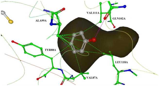
Contact map of the 1LI2 protein-ligand complex binding region. Hydrophobic contacts are shown as green dashed lines and the one hydrogen bond is shown as a pink dashed line. The binding pocket cavity is shown in dark yellow.

Judging from the crystal structure, phenol forms a hydrogen bond with GLN102A, and several hydrophobic contacts with VAL87A, TYR88A, ALA99A, VAL111A and LEU118A in the binding pocket (shown in Figure 4).

There are two atom types (sp³ oxygen and aromatic carbon atoms) in phenol. Based on the MT KECSA calculation, heat maps for both of the atom types within the binding pocket can be generated (Figure 5).

Figure 5.

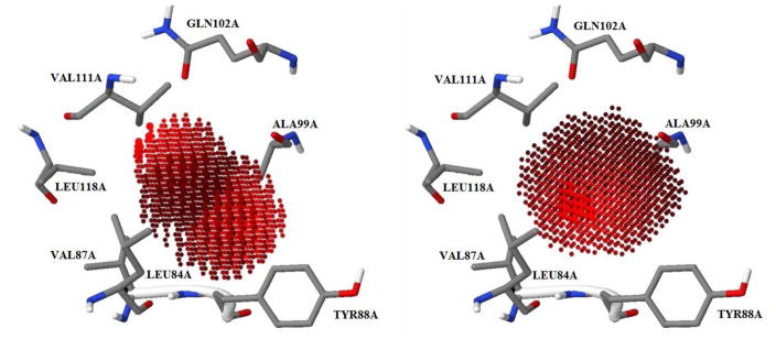
Heat maps for sp³ oxygen (left) and aromatic carbon (right). Grid points with lighter color indicate energetically favorable locations for certain atom types within the binding pocket.

The heatmap docking program then generated one sp³ oxygen and six aromatic carbons to their optimized position following the gradients on their corresponding energy heatmaps while satisfying the linkage constraints of phenol. As a result, together with the energetic global minimum ligand pose (GM), three more local minimum poses (pose a, b and c) were generated using the heatmap docking method. RMSD values (Å) and binding scores (pK_d) are shown in Table 2.

Table 2.

RMSD values (Å) and binding scores (pK_d) of the global and local minima.

	RMSD (Å)	Binding Affinity (pKd)
Global Minimum	0.937	3.329
Local Minimum a	2.667	2.255
Local Minimum b	2.839	2.975
Local Minimum c	2.342	3.299

As can be seen in Figure 6, the GM pose slightly deviates from the crystal structure (CS) because of the adjustment of the hydrogen bond distance between the phenol oxygen and the sp² oxygen on GLN102A in the MT KECSA calculation. The phenol benzene ring balances the contacts with ALA99A and TYR88A on one side and the contacts with LEU118A, VAL87A and LEU84A on the other. The local minimum pose c and b have close binding scores when compared to the GM pose. They form hydrogen bonds with different hydrogen acceptors (ALA99A backbone oxygen for pose c and LEU84A backbone oxygen for pose b) while maintaining very similar benzene ring locations. The local minimum pose a is trying to form a hydrogen bond with ALA99A backbone oxygen. However, the benzene ring of local minimum pose a is tilted towards the LEU118A, VAL87A and LEU84A side chain carbons, weakening the hydrogen bond with the ALA99A backbone oxygen with the net result being a reduction in binding affinity.

Figure 6.

In the binding pocket of protein-ligand complex 1LI2, ligand crystal structure (marked as CS) is shown as a stick & ball, the global minimum pose (marked as GM) is shown as a stick along with the three other identified local minimum (marked as a, b, and c). Red bubbles on the protein atoms indicate potential contacts with the ligand sp³ oxygen. Grey bubbles on the protein atoms indicate potential contacts with aromatic carbons.

Further Validation of the “Movable Type” Method

Using the MT method a further docking study was carried out on the test set of 795 protein-ligand complexes. In addition, in order to better evaluate the performance of MT scoring and heatmap docking, we also carried out a Glide scoring and docking study for comparison. ^{44, 45, 46}

For the Glide docking and scoring study, protein structures were prepared with the Protein Preparation Wizard utility of the Schrodinger 2013–2 Suite using Epik state penalties.^44,47 Protonation states were assigned using PROPKA at pH 7.0.^48,49 Hydrogen positions were optimized with OPLS 2005.^50,51 All the crystal waters were removed. Docking runs using the Glide version 5.9 Standard Precision (SP) and Extra Precision (XP) algorithms followed the preparation step.

The MT heatmap docking generated an average RMSD of 1.97Å with a 1.27Å standard deviation when compared to the protein-ligand crystal structure while Glide SP docking generated an average RMSD of 2.07Å with a 2.72Å standard deviation, Glide XP docking generated an average RMSD of 1.87Å with a 2.01Å standard deviation against the same set (Table 3.). The result for each individual system studied herein is given in the supplementary information. Based on this test result, MT heatmap docking showed a comparable performance to Glide results, all of which have ~2.0Å RMSD results. However, the standard deviation of the pose RMSD generated using heatmap docking is in a more narrow range than what is seen using SP and XP Glide.

Table 3.

RMSD values (Å) and standard deviations of RMSD (Å) from the MT heatmap docking results, compared with Glide SP and Glide XP results.

	RMSD (Å)	RMSD standard deviation (Å)
MT KECSA	1.97	1.27
Glide SP	2.07	2.72
Glide XP	1.87	2.01

We also compared the binding affinity computed by the MT method (actually pK_d/pK_i values) with the Glide SP and XP scores. We show the Glide scores vs. the experimental pK_d or pK_i values across the 795 protein-ligand complexes in the test set in Figure 7, together with the calculated pK_d or pK_i values from MT KECSA and the original KECSA model vs. the experimental pK_d or pK_i values of the same test set for comparison. Due to the different scales used by MT KECSA and the Glide scores, the comparison only includes Pearson’s r and Kendall τ values. MT KECSA and the original KECSA, as discussed above, generated Pearson’s r’s of 0.72 and 0.62, Kendall τ’s of 0.53 and 0.46. Glide SP yields a Pearson’s r of 0.46 and a Kendall τ of 0.52, while Glide XP yields a Pearson’s r of 0.42 and a Kendall τ of 0.29. Overall, we conclude that MT KECSA shows advantages over scoring with Glide.

Figure 7.

Plot of MT KECSA (A), the original KECSA model (B) calculated pK_d or pK_i values, Glide SP score (C) and Glide XP score (D) vs. Experimental pK_d or pK_i values.

Conclusions

The prediction of the free energies associated with a wide range of biological problems remains a very daunting task. Balancing the sampling of the relevant degrees of freedom with accurate energy computation makes this a very difficult problem. Herein we describe a new approach that in one-shot samples all the relevant degrees of freedom in a defined region directly affording a free energy without resorting to ad hoc modeling of the entropy associated with a given process. This is accomplished by converting ensemble assembly from a 3-D to a 1-D problem by using pairwise energies of all relevant interactions in a system coupled with their probabilities. We call this approach the moveable type (MT) method and in conjunction with Knowledge-based and Empirical Combined Scoring Algorithm (KECSA) potential function we demonstrated the application of this approach to protein ligand pose and binding free energy prediction. The resultant MT-KECSA model out-performs the original KECSA model showing the power of this approach. Importantly, the present MT model can be applied to any pairwise decomposable potential which will allow us to attack a wide range of problems in biology including the validation of potential functions.

References

- 1.Jorgensen WL, Tirado-Rives J. Monte Carlo vs. molecular dynamics for conformational sampling. J Phys Chem. 1996;100:14508. [Google Scholar]
- 2.Cancès E, Legoll F, Stoltz G. Theoretical and numerical comparison of some sampling methods for molecular dynamics. ESAIM, Math Model Numer Anal. 2007;41:351. [Google Scholar]
- 3.Gallicchio E, Levy RM. Advances in all atom sampling methods for modeling protein-ligand binding affinities. Curr Opin Struct Biol. 2011;21:161. doi: 10.1016/j.sbi.2011.01.010. [DOI] [PMC free article] [PubMed] [Google Scholar]
- 4.Halperin I, Ma B, Wolfson H, Nussinov R. Principles of docking: An overview of search algorithms and a guide to scoring functions. Proteins. 2002;47:409. doi: 10.1002/prot.10115. [DOI] [PubMed] [Google Scholar]
- 5.Limongelli V, Marinelli L, Cosconati S, La Motta C, Sartini S, Mugnaini L, Da Settimo F, Novellino E, Parrinello M. Sampling protein motion and solvent effect during ligand binding. Proc Natl Acad Sci U S A. 2012;109:1467. doi: 10.1073/pnas.1112181108. [DOI] [PMC free article] [PubMed] [Google Scholar]
- 6.Clark M, Guarnieri F, Shkurko I, Wiseman J. Grand Canonical Monte Carlo Simulation of Ligand-Protein Binding. J Chem Inf Model. 2006;46:231. doi: 10.1021/ci050268f. [DOI] [PubMed] [Google Scholar]
- 7.Okamoto Y. Generalized-ensemble algorithms: enhanced sampling techniques for Monte Carlo and molecular dynamics simulations. J Mol Graphics Modell. 2004;22:425. doi: 10.1016/j.jmgm.2003.12.009. [DOI] [PubMed] [Google Scholar]
- 8.Hendlich M, Lackner P, Weitckus S, Floeckner H, Froschauer R, Gottsbacher K, Casari G, Sippl MJ. Identification of native protein folds amongst a large number of incorrect models. The calculation of low energy conformations from potentials of mean force. J Mol Biol. 1990;216:167. doi: 10.1016/S0022-2836(05)80068-3. [DOI] [PubMed] [Google Scholar]
- 9.Jones-Hertzog DK, Jorgensen WL. Binding affinities for sulfonamide inhibitors with human thrombin using Monte Carlo simulations with a linear response method. J Med Chem. 1997;40:1539. doi: 10.1021/jm960684e. [DOI] [PubMed] [Google Scholar]
- 10.Shaw DE, Maragakis P, Lindorff-Larsen K, Piana S, Dror RO, Eastwood MP, Bank JA, Jumper JM, Salmon JK, Shan Y, Wriggers W. Atomic-Level Characterization of the Structural Dynamics of Proteins. Science. 2010;330:341. doi: 10.1126/science.1187409. [DOI] [PubMed] [Google Scholar]
- 11.Kannan S, Zacharias M. Simulated annealing coupled replica exchange molecular dynamics—An efficient conformational sampling method. J Struct Biol. 2009;166:288. doi: 10.1016/j.jsb.2009.02.015. [DOI] [PubMed] [Google Scholar]
- 12.Klepeis JL, Lindorff-Larsen K, Dror RO, Shaw DE. Long-timescale molecular dynamics simulations of protein structure and function. Curr Opin Struct Biol. 2009;19:120. doi: 10.1016/j.sbi.2009.03.004. [DOI] [PubMed] [Google Scholar]
- 13.Schlick T. Molecular dynamics-based approaches for enhanced sampling of long-time, large-scale conformational changes in biomolecules. F1000 Biol Rep. 2009;1:51. doi: 10.3410/B1-51. [DOI] [PMC free article] [PubMed] [Google Scholar]
- 14.Bonomi M, Branduardi D, Bussi G, Camilloni C, Provasi D, Raiteri P, Donadio D, Marinelli F, Pietrucci F, Broglia RA, Parrinello M. PLUMED: A portable plugin for free-energy calculations with molecular dynamics. Comput Phys Commun. 2009;180:1961. [Google Scholar]
- 15.Gilson MK, Zhou HX. Calculation of Protein-Ligand Binding Affinities. Annu Rev Biophys Biomol Struct. 2007;36:21. doi: 10.1146/annurev.biophys.36.040306.132550. [DOI] [PubMed] [Google Scholar]
- 16.Karney CF, Ferrara JE, Brunner S. Method for computing protein binding affinity. J Comput Chem. 2005;26:243. doi: 10.1002/jcc.20167. [DOI] [PubMed] [Google Scholar]
- 17.Michel J, Essex JW. Prediction of protein-ligand binding affinity by free energy simulations: assumptions, pitfalls and expectations. J Comput-Aided Mol Des. 2010;24:639. doi: 10.1007/s10822-010-9363-3. [DOI] [PubMed] [Google Scholar]
- 18.Sippl MJ. Calculation of conformational ensembles from potentials of mena force: an approach to the knowledge-based prediction of local structures in globular proteins. J Mol Biol. 1990;213:859. doi: 10.1016/s0022-2836(05)80269-4. [DOI] [PubMed] [Google Scholar]
- 19.Tuffery P, Derreumaux P. Flexibility and binding affinity in protein-ligand, protein-protein and multi-component protein interactions: limitations of current computational approaches. J R Soc Interface. 2012;9:20. doi: 10.1098/rsif.2011.0584. [DOI] [PMC free article] [PubMed] [Google Scholar]
- 20.Fan H, Schneidman-Duhovny D, Irwin JJ, Dong G, Shoichet BK, Sali A. Statistical potential for modeling and ranking of protein-ligand interactions. J Chem Inf Model. 2011;51:3078. doi: 10.1021/ci200377u. [DOI] [PMC free article] [PubMed] [Google Scholar]
- 21.Gohlke H, Hendlich M, Klebe G. Knowledge-based scoring function to predict protein-ligand interactions. J Mol Biol. 2000;295:337. doi: 10.1006/jmbi.1999.3371. [DOI] [PubMed] [Google Scholar]
- 22.Huang SY, Zou X. An iterative knowledge-based scoring function to predict protein- ligand interactions: II. Validation of the scoring function. J Comput Chem. 2006;27:1876. doi: 10.1002/jcc.20505. [DOI] [PubMed] [Google Scholar]
- 23.Huang SY, Zou X. Advances and challenges in protein-ligand docking. Int J Mol Sci. 2010;11:3016. doi: 10.3390/ijms11083016. [DOI] [PMC free article] [PubMed] [Google Scholar]
- 24.Huang SY, Zou X. Inclusion of Solvation and Entropy in the Knowledge-Based Scoring Function for Protein-Ligand Interactions. J Chem Inf Model. 2010;50:262. doi: 10.1021/ci9002987. [DOI] [PMC free article] [PubMed] [Google Scholar]
- 25.Muegge I, Martin YC. A general and fast scoring function for protein-ligand interactions: a simplified potential approach. J Med Chem. 1999;42:791. doi: 10.1021/jm980536j. [DOI] [PubMed] [Google Scholar]
- 26.Muegge I. A knowledge-based scoring function for protein-ligand interactions: Probing the reference state. Perspect Drug Discovery Des. 2000;20:99. [Google Scholar]
- 27.Muegge I. Effect of ligand volume correction on PMF scoring. J Comput Chem. 2001;22:418. [Google Scholar]
- 28.DeWitte RS. Shakhnovich, E. I. SMoG: de Novo design method based on simple, fast, and accutate free energy estimate. 1. Methodology and supporting evidence. J Am Chem Soc. 1996;118:11733. [Google Scholar]
- 29.Velec HF, Gohlke H, Klebe G. DrugScore(CSD)-knowledge-based scoring function derived from small molecule crystal data with superior recognition rate of near-native ligand poses and better affinity prediction. J Med Chem. 2005;48:6296. doi: 10.1021/jm050436v. [DOI] [PubMed] [Google Scholar]
- 30.Zheng Z, Merz KM., Jr Ligand identification scoring algorithm (LISA) J Chem Inf Model. 2011;51:1296. doi: 10.1021/ci2000665. [DOI] [PMC free article] [PubMed] [Google Scholar]
- 31.Benson ML, Faver JC, Ucisik MN, Dashti DS, Zheng Z, Merz KM., Jr Prediction of trypsin/molecular fragment binding affinities by free energy decomposition and empirical scores. J Comput-Aided Mol Des. 2012;26:647. doi: 10.1007/s10822-012-9567-9. [DOI] [PubMed] [Google Scholar]
- 32.Faver JC, Zheng Z, Merz KM., Jr Model for the fast estimation of basis set superposition error in biomolecular systems. J Chem Phys. 2011;135:144110. doi: 10.1063/1.3641894. [DOI] [PMC free article] [PubMed] [Google Scholar]
- 33.Faver JC, Zheng Z, Merz KM., Jr Statistics-based model for basis set superposition error correction in large biomolecules. Phys Chem Chem Phys. 2012;14:7795. doi: 10.1039/c2cp23715f. [DOI] [PubMed] [Google Scholar]
- 34.Faver JC, Yang W, Merz KM., Jr The Effects of Computational Modeling Errors on the Estimation of Statistical Mechanical Variables. J Chem Theory Comput. 2012;8:3769. doi: 10.1021/ct300024z. [DOI] [PMC free article] [PubMed] [Google Scholar]
- 35.Zheng Z, Merz KM., Jr Development of the Knowledge-Based and Empirical Combined Scoring Algorithm (KECSA) To Score Protein–Ligand Interactions. J Chem Inf Model. 2013;53:1073. doi: 10.1021/ci300619x. [DOI] [PMC free article] [PubMed] [Google Scholar]
- 36.Wang R, Fang X, Lu Y, Wang S. The PDBbind database: collection of binding affinities for protein-ligand complexes with known three-dimensional structures. J Med Chem. 2004;47:2977. doi: 10.1021/jm030580l. [DOI] [PubMed] [Google Scholar]
- 37.Wang R, Fang X, Lu Y, Yang CY, Wang S. The PDBbind database: methodologies and updates. J Med Chem. 2005;48:4111. doi: 10.1021/jm048957q. [DOI] [PubMed] [Google Scholar]
- 38.Goodsell DS, Morris GM, Olson AJ. Automated docking of flexible ligands: applications of AutoDock. J Mol Recognit. 1996;9:1. doi: 10.1002/(sici)1099-1352(199601)9:1<1::aid-jmr241>3.0.co;2-6. [DOI] [PubMed] [Google Scholar]
- 39.Leis S, Zacharias M. Efficient inclusion of receptor flexibility in grid-based protein- ligand docking. J Comput Chem. 2011;32:3433. doi: 10.1002/jcc.21923. [DOI] [PubMed] [Google Scholar]
- 40.Taylor RD, Jewsbury PJ, Essex JW. A review of protein-small molecule docking methods. J Comput-Aided Mol Des. 2002;16:151. doi: 10.1023/a:1020155510718. [DOI] [PubMed] [Google Scholar]
- 41.Wu G, Robertson DH, Brooks CL, 3rd, Vieth M. Detailed analysis of grid-based molecular docking: A case study of CDOCKER-A CHARMm-based MD docking algorithm. J Comput Chem. 2003;24:1549. doi: 10.1002/jcc.10306. [DOI] [PubMed] [Google Scholar]
- 42.Kubinyi H. Comparative molecular field analysis (CoMFA) Handbook of Chemoinformatics: From Data to Knowledge in 4 Volumes. 2008:1555. [Google Scholar]
- 43.Goodford PJ. A computational procedure for determining energetically favorable binding sites on biologically important macromolecules. J Med Chem. 1985;28:849. doi: 10.1021/jm00145a002. [DOI] [PubMed] [Google Scholar]
- 44.Friesner RA, Banks JL, Murphy RB, Halgren TA, Klicic JJ, Mainz DT, Repasky MP, Knoll EH, Shelley M, Perry JK. Glide: a new approach for rapid, accurate docking and scoring. 1. Method and assessment of docking accuracy. J Med Chem. 2004;47:1739. doi: 10.1021/jm0306430. [DOI] [PubMed] [Google Scholar]
- 45.Halgren TA, Murphy RB, Friesner RA, Beard HS, Frye LL, Pollard WT, Banks JL. Glide: a new approach for rapid, accurate docking and scoring. 2. Enrichment factors in database screening. J Med Chem. 2004;47:1750. doi: 10.1021/jm030644s. [DOI] [PubMed] [Google Scholar]
- 46.Friesner RA, Murphy RB, Repasky MP, Frye LL, Greenwood JR, Halgren TA, Sanschagrin PC, Mainz DT. Extra Precision Glide: Docking and Scoring Incorporating a Model of Hydrophobic Enclosure for Protein-Ligand Complexes. J Med Chem. 2006;49:6177. doi: 10.1021/jm051256o. [DOI] [PubMed] [Google Scholar]
- 47.Sastry GM, Adzhigirey M, Day T, Annabhimoju R, Sherman W. Protein and ligand preparation: parameters protocols and influence on virtual screening enrichments. J Comput Aided Mol Des. 2013;27:221. doi: 10.1007/s10822-013-9644-8. [DOI] [PubMed] [Google Scholar]
- 48.Rostkowski M, Olsson MH, Søndergaard CR, Jensen JH. Graphical analysis of pH-dependent properties of proteins predicted using PROPKA. BMC Struct Biol. 2011;11:6. doi: 10.1186/1472-6807-11-6. [DOI] [PMC free article] [PubMed] [Google Scholar]
- 49.Olsson MHM, Søndergard CR, Rostkowski M, Jensen JH. PROPKA3: Consistent Treatment of Internal and Surface Resi- dues in Empirical pKa predictions. J Chem Theor Comput. 2011;7:525. doi: 10.1021/ct100578z. [DOI] [PubMed] [Google Scholar]
- 50.Jorgensen WL, Tirado-Rives J. The OPLS [optimized potentials for liquid simulations] potential functions for proteins, energy minimizations for crystals of cyclic peptides and crambin. J Am Chem Soc. 1988;110:1657. doi: 10.1021/ja00214a001. [DOI] [PubMed] [Google Scholar]
- 51.Kaminski GA, Friesner RA, Tirado-Rives J, Jorgensen WL. Evaluation and reparametrization of the OPLS-AA force field for proteins via comparison with accurate quantum chemical calculations on peptides. J Phys Chem B. 2001;105:6474. [Google Scholar]
Associated Data
This section collects any data citations, data availability statements, or supplementary materials included in this article.