Introducing Charge Hydration Asymmetry into the Generalized Born Model

Abstract

The effect of charge hydration asymmetry (CHA)—non-invariance of solvation free energy upon solute charge inversion—is missing from the standard linear response continuum electrostatics. The proposed charge hydration asymmetric–generalized Born (CHA–GB) approximation introduces this effect into the popular generalized Born (GB) model. The CHA is added to the GB equation via an analytical correction that quantifies the specific propensity of CHA of a given water model; the latter is determined by the charge distribution within the water model. Significant variations in CHA seen in explicit water (TIP3P, TIP4P-Ew, and TIP5P-E) free energy calculations on charge-inverted “molecular bracelets” are closely reproduced by CHA–GB, with the accuracy similar to models such as SEA and 3D-RISM that go beyond the linear response. Compared against reference explicit (TIP3P) electrostatic solvation free energies, CHA–GB shows about a 40% improvement in accuracy over the canonical GB, tested on a diverse set of 248 rigid small neutral molecules (root mean square error, rmse = 0.88 kcal/mol for CHA–GB vs 1.24 kcal/mol for GB) and 48 conformations of amino acid analogs (rmse = 0.81 kcal/mol vs 1.26 kcal/mol). CHA–GB employs a novel definition of the dielectric boundary that does not subsume the CHA effects into the intrinsic atomic radii. The strategy leads to finding a new set of intrinsic atomic radii optimized for CHA–GB; these radii show physically meaningful variation with the atom type, in contrast to the radii set optimized for GB. Compared to several popular radii sets used with the original GB model, the new radii set shows better transferability between different classes of molecules.

1. Introduction

The conceptual simplicity of the implicit solvation (solvent treated as a structureless continuum dielectric medium) framework¹⁻⁴ facilitates fast quantitative estimates of solvation effects that are key in biomolecular computation. In this framework, one often approximates the solvation free energy—free energy change to transfer a solute from gas phase to aqueous phase—as a sum of its electrostatic (polar) and non-polar parts, that is, ΔG_solv = ΔG_pol + ΔG_np. Among these, ΔG_pol is by far the largest contribution in the majority of molecules; ΔG_np has not been the computational bottleneck so far, perhaps due to the simplistic nature of the popular approximations most commonly used in this context.⁵ The defacto “workhorse” for estimation of ΔG_pol in most practical computations is the linear response continuum treatment of electrostatics based on numerical solutions of the Poisson (PE) or Poisson–Boltzmann (PB) equation,³ or the generalized Born (GB) model,⁴ which is an approximation to the PE. Because of its closed analytical form, the GB is arguably the fastest among these implicit solvent models. Some noteworthy applications of GB include protein folding,⁶⁻¹⁵ “large scale” motions in biomolecules,¹⁶⁻¹⁸ analysis of nucleic acid conformational energetics,^19,20 binding between proteins and nucleic acids,²¹⁻²³ modeling of peptides in membrane environment,²⁴⁻²⁸ and many others.²⁹⁻³²

A number of approximations of various severity separate the linear response continuum PE/PB or GB models from the more accurate explicit solvent treatment.³³ One such serious approximation is the neglect of charge hydration asymmetry (CHA)³⁴⁻⁴¹—the characteristic dependence of solvation free energy, ΔG_solv, on the sign of the charges in a solute. The effect is clearly missing from the linear response continuum model, in which ΔG_solv ∼ q²/R for a single spherical charge q of radius R. A straightforward example of CHA is the large difference between experimental ΔG_solv for oppositely charged ions of similar ionic radius; for example, K⁺ and F^–42,43 differ roughly by 50 kcal/mol, which is about 50% of their individual ΔG_solv values.

Within the continuum framework, experimental solvation energies of single-charge spherical ions could be reproduced accurately by ad hoc adjustments made to the ion radii.^44,45 These adjustments essentially amount to redefining the dielectric boundary, which (to an extent) implicitly accounts for the missing CHA by making the boundary depend on the ion charge. While for single ions the procedure works well, its generalization to the multi-atom case did not yet lead to a single consensus⁴⁶ set of atomic radii; a set that works well for a certain class of molecules does not necessarily perform equally well for a different class of structures (see, for example, Table 1). We argue that to a significant degree the problem is the missing CHA; we show that once the effect is explicitly added into even the simplest of the continuum models, the GB, a more universal set of atomic radii can be developed. Several existing “beyond PE” semi-empirical approaches such as the semi-explicit assembly (SEA)⁵¹ (assembling hydration shells of solutes using the precomputed properties of hydration shells of charged spheres in explicit solvent) or integral equations based reference interaction site models (RISM, 3D-RISM)⁵²⁻⁵⁵ already implicitly account for CHA, along with many other effects missing from the linear response continuum framework. However, these methods are not comparable to the GB model in computational efficiency and conceptual simplicity, which gives us an additional motivation to attempt to introduce CHA directly into the GB model.

Table 1. Root Mean Square Error (rmse, in kcal/mol) of the GB ΔG_pol Relative to the Explicit Solvent (TIP3P) Reference^a.

radii set	small molecules	amino acid analogs
Bondi48 (10)	1.55	1.99
Parse49 (10)	2.33	7.45
ZAP950 (13)	0.82	2.88

^aThe numerical R6 GB calculations⁴⁷ (see Methods) are based on three common sets of atomic radii;⁴⁸⁻⁵⁰ the number of atom types for each radius set is shown in parentheses. The corresponding errors in numerical PE ΔG_pol (not shown) are not smaller.

Elsewhere,⁵⁶ we presented a derivation of a CHA-aware analogue of the Born equation,⁵⁷ which can be regarded as a single spherical charge limit of the generalized Born approximation. A key novelty of our approach lies in a distinct separation between the placement of the solute dielectric boundary and the manner in which one accounts for the asymmetric response of the solvent (water) to the sign of the solute charge. Within the approach, the CHA effects no longer have to be mimicked by a redefinition of the dielectric boundary via ad hoc adjustments to the atomic radii. Instead, the asymmetric response is accounted for by a scaling factor applied to the Born electrostatic solvation energy; the scaling contains the details of the asymmetric response specific to the water model one wants to emulate. Here, we apply the strategy to derive a CHA-aware analogue of the GB equation, which we call the charge hydration asymmetric–generalized Born (CHA–GB) model. By direct comparison with explicit solvation energies, we will show how CHA–GB improves the accuracy of the GB framework. The new model was also compared with several other recent semi-continuum models such as SEA⁵¹ and 3D-RISM.⁵²⁻⁵⁵

2. Charge Hydration Asymmetric–Generalized Born: CHA–GB

The “CHA-aware” modified Born formula for a single spherical ion of radius ρ and charge q is given by⁵⁶

1

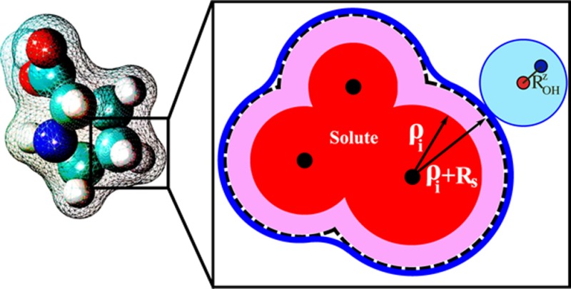
where ε_in and ε_out are dielectric constants of the solute and the solvent, respectively, and ρ_w = 1.4 Å is the water probe radius. The first part in eq 1 describes the charge-symmetric dielectric response of the original Born equation,⁵⁷ accurate in the limit of a continuum “charge-symmetric” solvent. (Throughout this article we will loosely use the word “symmetric” for models devoid of charge hydration asymmetry.) One such model is the mean spherical approximation⁵⁸ (MSA) for which the Born model is exact; the dielectric boundary is shifted up by R_s = 0.52 Å relative to the surface of the spherical solute of radius ρ. Later in this work, we will extend this dielectric boundary definition to solutes. Once the charge-symmetric solvation is accounted for in the “Symmetric Born” part of eq 1, the charge hydration asymmetry (CHA) correction enters via a multiplicative scaling factor η. In η, the CHA of a water model being emulated is controlled by the model dependent parameter R_OH^z = Q̃_zz/p, where Q̃_zz and p are respectively the primitive (non-traceless) quadrupole and dipole moments of the n-point water model (Table 2).

Table 2. R_OH^z = Q̃_zz/p for the Three Water Models Used in This Work^a.

^aQ̃_zz = ∑_iq_iz_i² and p = q_iz_i, where z_i is the azimuthal-symmetry coordinate of charge q_i with respect to the molecule center. A geometric interpretation of R_OH for the TIP3P water model is shown in the schematic on the right.

We now seek an analogue of the CHA-aware Born equation, eq 1, for molecules. Without the CHA, such analogue is well known—the canonical (charge-symmetric) generalized Born (GB) equation

2

where q_i(j) is the atomic partial charge of atom i(j). The empirical function f_ij^GB is

3

where r_ij is the distance between the i^th and j^th atom, and R_i and R_j are their effective Born radii. The effective Born radius of an atom characterizes its degree of burial inside the solute. Many efficient methods exist for computing this quantity (see ref (33) for a recent review).

The generalized Born approximation can be viewed as an interpolation between the two limiting cases: case (a) r_ij → ∞, that is, charged atoms are treated as separate distant (non-interacting) charged spheres and case (b) r_ij → 0, that is, all charges merge to form a single sphere of charge ∑_iq_i and effective Born radius R. The empirical correction, exp(−r_ij²/(4R_iR_j)) in f_ij, eq 3, originally introduced by Still et al.,⁵⁹ performs the interpolation in a way that at least partially accounts for non-spherical shapes of realistic molecules.⁴ Our strategy is to utilize the same interpolation to derive the CHA-aware analogue of eq 2 by matching the asymptotes, (a) and (b), to the CHA-aware Born formula (eq 1). In what follows, we consider these two limiting cases in detail.

Case (a): From eq 2, the ΔG_pol = (−1/2)(1/ε_in – 1/ε_out)∑_i(q_i²/R_i), that is, the sum of self-energies of every atom in the molecule. Comparing with the symmetric Born part of eq 1, the effective Born radius, R_i, is seen as equivalent to the dielectric boundary radius, ρ + R_s. To add CHA correction in this limit, we scale each GB self-energy term by the corresponding η_i = {1+sgn[q_i]R_OH/(R_i – R_s + ρ_w)}⁻¹ from eq 1. This implies ΔG_pol → (−1/2)(1/ε_in – 1/ε_out)∑_i(q_i²/R_i)η_i as r_ij → ∞.

Case (b): In this limit, all the charges are merged together to form a single sphere of effective Born radius, R, with the total charge of ∑_iq_i. Using charge-symmetric eq 2, we can write ΔG_pol = (−1/2)(1/ε_in – 1/ε_out)(∑_iq_i)²/R. To add the CHA according to eq 1, the overall ΔG_pol must now be scaled with the CHA factor that depends upon the net charge of the molecule, that is, η = {1 + sgn[Σ_iq_i]R_OH^z/(R – R_s + ρ_w)}⁻¹. This implies ΔG_pol → (−1/2)(1/ε_in – 1/ε_out){∑_i(q_i)/R}η as r_ij → 0.

In short, for case (a), each self-term of eq 2 has to be scaled by its respective CHA scaling factor, whereas for case (b), a global CHA-scaling is needed. To consistently satisfy both of these asymptotes while preserving the overall GB functional form set by eqs 2 and 3, we need a single functional form for the CHA scaling factor η_i that is aware of other charges in the molecule. To this end, we make η_i a function of ∑_jq_je^{–τr_ij2/(R_iR_j)} and scale the effective Born radii accordingly

4

where τ is a positive constant that controls the effective range of the neighboring charges (j) affecting the CHA of atom (i). For realistic molecules, the r_ij’s are of the same order of R_i’s, and hence, it can be argued that τ is of the order of 1. Indeed, the value of τ that we obtain by systematic fitting against explicit solvent reference ΔG_pol’s (see Methods) is close to 1. Using eq 4, the charge hydration asymmetric–generalized Born (CHA–GB) approximation can be written as

5

where f_ij^CHA–GB = (r_ij + R̃_iR̃_j exp (−r_ij²/(4R_iR_j)))^1/2. In line with our philosophy of separating the CHA effects from the purely geometric dielectric boundary, we do not use the CHA-corrected effective radii in the exp (−r_ij/(4R_iR_j)) factor due to its “geometry correction” role in the GB model.

Charge-Symmetric Dielectric Boundary

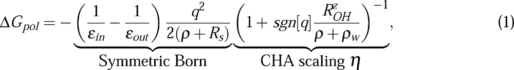
The dielectric boundary, which separates the low dielectric solute from the high dielectric solvent, is a key concept in the standard continuum solvation approach. Just like in the original GB model, the boundary is needed in our CHA–GB formalism for the computation of the effective Born radii via an integral over the solute surface (see Methods). The dielectric boundary definition we propose, Figure 1, is a generalization of the single spherical ion case, eq 1, designed to account for the charge-symmetric part of the solvent dielectric response. The idea is to make the boundary manifestly invariant to inversion of charges within the solute, as is the case in the classical macroscopic continuum electrostatics framework⁶⁰ on which the GB or PE are based. Charge hydration asymmetry of a more realistic solvent has to be added as an external correction to electrostatic solvation energy, for example, as done above for the case of the proposed CHA–GB formalism. A sharp dielectric boundary is defined by a set of atomic radii and the rolling probe radius. In principle, one could find a set of optimal charge-symmetric atomic radii ρ_i by an optimization against solvation energies computed within a charge-symmetric explicit water model such as BNS⁶¹ or an even simpler model in which the appropriate point dipole is placed at a single vdW center.⁵⁶ In practice, we will first add CHA via eqs 4 and 5, and then iteratively optimize the radii to obtain best fit against a more realistic charge-asymmetric explicit solvent (TIP3P) ΔG_pol for a representative set of realistic molecules.

Figure 1.

Charge-symmetric dielectric boundary used in CHA–GB for multi-atom solutes. The schematic inset shows the key construction steps. Each atomic radius (ρ_i, red circle) is increased (purple area) by the same correction R_s = 0.52 Å. The dielectric surface (blue line) is outlined by rolling a probe of radius ρ_w – R_s. The smaller than the standard ρ_w = 1.4 Å probe ensures invariance of the solvent accessible surface around the solute.

3. Methods

Molecule Sets

Four molecule sets^38,62−64 were used to test the performance of the proposed model.

Set 1: This is a polar solute series³⁸ of several “bracelet”-like regular planar polygonal (triangle to octagon) molecules made with a single aromatic carbon “ca” atom type (Figure 2). These charge-inverted bracelets were specifically designed to study solvent-dependent CHA effects.³⁸ Two charge configurations for each molecular geometry were considered, the N and P bracelets, that is, one atom in the molecule charged −1e (N bracelet) or +1e (P bracelet), whereas the rest of the atoms were equally charged such that the overall molecule is neutral. The explicit ΔG_pol in TIP3P and TIP4P-Ew were obtained using standard thermodynamic integration (TI)⁶⁵ in Amber 12,⁶⁶ whereas the TIP5P-E ΔG_pol were deduced from ref (38) (Supporting Information).

Figure 2.

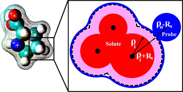
Polar solvation free energies of the charged-inverted “bracelets”. Atomic structures of the N-bracelets are shown on the top horizontal axis, while the P-bracelets are shown at the bottom. Explicit solvent energies for three different water models ((a)TIP4P-Ew, (b)TIP3P, and (c)TIP5P-E) are denoted by red dots for N-bracelets and blue dots for P-bracelets. The corresponding CHA–GB energies are shown by the black triangles; the R_OH^z parameter that controls the propensity for CHA in CHA–GB, eq 5, is set to the value appropriate for the given explicit water model (Table 2).

Set 2: A set of 248 rigid diverse neutral small molecules was selected from a larger set of 504 molecules commonly used to test solvent models;^47,51,62,67 the corresponding explicit water (TIP3P) ΔG_pol values were taken from ref (62). The rationale for focusing on the rigid molecules is as follows. It is well known that solvation free energies are sensitive to the solute conformations;⁶⁷ poor conformational sampling may lead to errors in estimated solvation energies relative to the experiment. However, our primary goal here is to improve the implicit solvent estimates of the polar part of solvation energy, and so we believe that a comparison with the single conformation polar solvation free energy in the explicit solvent is the best strategy. That is, we would like to minimize the number of other factors that affect the ΔG_pol estimates. In order to compare with the explicit ΔG_pol, we therefore chose the most rigid 248 molecules that showed small conformational variability during the molecular dynamics simulations performed on the same 504 molecule set as in ref (67) (see the Supporting Information for details).

Set 3: This is a set of 48 structures of single amino acid analogs of the form N-acetyl-X-N′-methylamide (X refers to one of the 20 amino acids). Among these, 40 structures were taken directly from ref (63), to which we added eight additional molecules by neutralizing the charged structures: ASP, LYS, GLU, and ARG (Supporting Information).

Set 4: A set of 19 neutral small protein structures with average sizes of 30 amino acid residues were randomly selected from a larger set used in ref (64) (Supporting Information).

Parameter Optimization: Realistic Molecule Sets

For CHA–GB, 10 parameters (ρ_i of nine atom types, Table 3, and τ = 1.47) were optimized against the explicit (TIP3P) solvation free energy with a training set comprised of 124 molecules from the rigid small molecule set and 24 molecules from the set of amino acid analogs. These molecules in the training set were sampled to approximate an equal representation of the span of solvation free energies as well as of the atom types of the entire set (Supporting Information). We used the Nelder–Mead simplex algorithm⁶⁸ with the objective function that weighs equally RMS deviations from the reference ΔG_pol of the small molecules and the amino acid analogs. Convergence to the optimum set of parameters (Table 3) was ensured within 100 independent runs with random initial guess parameters (within a physical range) (Supporting Information). For all realistic molecules, we use the analytical linearized Poisson–Boltzmann (ALPB) model,⁶⁹ which is a correction to GB, eq 2, that introduces a physically correct dependence on the dielectric constants while keeping the computational efficiency of the original. In ALPB, ΔG_pol is approximated as

6

where β = ε_in/ε_out, α = 0.571412, and A is the electrostatic size of the molecule, essentially the overall size of the structure computed analytically.⁶⁹ We add the CHA correction to ALPB by replacing f_ij^GB by f_ij similar to eq 5. To avoid uncertainties associated with the effective Born radii estimation, we use numerical “R6” radii,⁷⁰ which were shown^47,71 to deliver ΔG_pol estimates essentially as accurate as those based on the perfect⁷² PE-based radii. Specifically, the effective radii are computed via

7

where r is the position of the infinitesimal surface element dS that encloses the charge-symmetric dielectric boundary ∂V (Figure 1), and r_i is the coordinate of atom i. Unless otherwise stated, for canonical GB, we use the Lee–Richards molecular surface⁷³ obtained with the standard water probe radius ρ_w = 1.4 Å. We use a numerical approximation of eq 7, representing the dielectric boundary as a triangulated mesh with density of 6 vertices/Ų obtained using MSMS⁷⁴ package. For proteins structures, following ref (71), we add a uniform correction of 0.028 Å^–1 to the R_i^–1 in eq 7.

Table 3. Optimized Intrinsic Atomic Radii Sets for CHA–GB and GB.

	radii set (Å)
	C	H	N	O	S	F	Cl	Br	I
CHA–GB	1.56	0.47	1.59	1.37	1.88	1.44	1.84	1.92	2.29
GB	1.76	1.29	1.46	1.50	2.04	1.16	1.25	2.04	1.72

Parameter Optimization: N and P Bracelets

The intrinsic radius of the aromatic carbon, “ca” atom type, was obtained by fitting against the TIP4P-Ew ΔG_pol – optimal ρ(“ca”) = 1.37 Å. The same value of τ = 1.47 as above was used in eq 4.

3D-RISM

We computed single point 3D-RISM ΔG_pol (TIP3P) using the implementation⁷⁵ in AMBER-12⁶⁶ with the protocol from http://dansindhikara.com/Tutorials/. These estimates were adjusted⁷⁶ by two parameters, a₁ and a₂, fit against the explicit solvent ΔG_pol

8

where ΔG_pol^3D-RISM/GF is the 3D-RISM ΔG_pol using the Kovalenko–Hirata closure⁷⁷ assuming Gaussian fluctuation of the solvent, ΔG_pol is the corrected polar solvation energy, V is the partial molar volume, and ρ = 0.0333A^–3 is the solvent number density. The optimized values of a₁ and a₂ are provided in the Supporting Information.

4. Performance of the New Model

CHA–GB closely reproduces the explicit polar solvation energy (ΔG_pol) (Figure 2) of the charge inverted N and P “bracelet” molecules in TIP3P (rmse = 0.67 kcal/mol), TIP4P-Ew (rmse = 1.02 kcal/mol), and TIP5P-E (rmse = 0.50 kcal/mol) water models emulated in CHA–GB by using the appropriate value of R_OH^z from Table 2. Note that using identical (for all water models) dielectric boundaries for the N and P bracelets of same size properly captures the propensity for CHA of each of the three explicit water models tested. It is interesting that within CHA–GB, the CHA contributions from both self-terms and cross terms in eq 5 are significant. For example, for TIP3P, the ratio of magnitude of CHA in cross terms to that in the self-terms, ⟨|ΔΔG_pol(cross)/ΔΔG_pol(self)|⟩ = 0.6. These contributions have opposite effects on the overall CHA; the CHA in self-terms is partially negated by the CHA in cross terms. As expected, the canonical GB does not capture the CHA (Figure 2a); the best fit to explicit solvent ΔG_pol results in very different values of ρ(“ca”) for different water models as the readjustment of the dielectric boundary compensates for the missing CHA. The inability of the Poisson treatment to capture CHA of the same “bracelet” molecules was noted earlier.³⁸ In contrast, our fairly simplistic way of introducing the CHA into the linear response continuum already captures the effect at a level similar to considerably more complex “beyond Poisson” models such as 3D-RISM^76,78 and SEA⁵¹ (Figure 3). A noteworthy observation is that the atomic radii optimized for CHA–GB have physically meaningful variations with the atom type (Table 3) unlike the ones optimal for GB that have ρ(I) < ρ(Br) and ρ(H) > ρ(Cl). It is also reassuring that the optimal hydrogen radius ρ(H) = 0.47 Å in the CHA–GB model is such that the realistic distance⁷⁹ of about 2 Å observed between the hydrogen and its electronegative partner in the hydrogen bond can now be reproduced. Compared against the reference (TIP3P) ΔG_pol, CHA–GB shows approximately 40% improvement in accuracy (root mean square error, rmse) over the canonical GB (Table 4) for the 248 small molecules and 48 amino acid analogs. The largest errors and the average errors are also reduced in the CHA–GB model. For small proteins, CHA–GB also shows an improvement in accuracy; note that this type of structure was not used to train the radii sets. Arguably, the most impressive achievement of CHA–GB is that it provides equally good accuracy of better than 1 kcal/mol simultaneously for both the small molecules and amino acid analogs. This is in contrast to GB. For example, GB with a ZAP9 set (13 atom types) specifically optimized for small molecules can yield similar good accuracy (ΔG_pol rmse = 0.82 kcal/mol) for the 248 small molecules, but then the corresponding errors for the 48 amino acid analogs become large (ΔG_pol rmse = 2.88 kcal/mol) (Table 1). We have checked directly that the uniformity of the accuracy improvement or equivalently the improved transferability of the new radii set is indeed the consequence of introducing the CHA into the GB model. Namely, even if the new dielectric boundary of Figure 1 is used in the charge-symmetric GB, the model still cannot reach the 1 kcal/mol rmse accuracy of ΔG_pol simultaneously for both the small molecules and amino acid analogs(Supporting Information). Our overall conclusions do not change, and the accuracy of CHA–GB remains essentially the same if we extend the molecule set to include the flexible molecules from the original set of 504 neutral molecules (Supporting Information). A comparison of the performance of CHA–GB and 3D-RISM⁷⁷ is presented in Table 5. Note that the same training set and optimization technique (see Methods and Supporting Information) was used to obtain best fit parameters for both models. A systematic comparison of CHA–GB with other “beyond PE” models is out of the scope here. However, we note that the published performance of the SEA⁵¹ model relative to the explicit solvent on the same set of 504 small molecules (same partial atomic charges) (ΔG_pol rmse = 0.81 kcal/mol) is comparable to that of CHA–GB (rmse = 0.89 kcal/mol).

Figure 3.

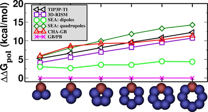
Asymmetry in the polar part of solvation free energies, ΔΔG_pol = |ΔG_pol(N) – ΔG_pol(P)| for N/P bracelets using different methods. For the SEA model, the data are adapted from ref (51).

Table 4. Accuracy of ΔG_pol Estimated by CHA–GB and GB Based on Their Respective Optimal Atomic Radii (Table 3)^a.

	small molecules		amino acid analogs		proteins
	GB	CHA–GB	GB	CHA–GB	GB	CHA–GB
rmse	1.24	0.88	1.26	0.81	10.24	8.95
⟨err⟩	–0.53	–0.37	0.24	0.09	–6.12	–2.80
⟨|err|⟩	0.93	0.63	0.90	0.64	7.79	7.63
r2	0.86	0.93	0.998	0.999	0.99	0.99
%(|err| > 2kBT)	30.6	14.9	25.0	16.7	84.2	89.5
rmse worst 5%	3.20	2.55	4.14	2.11	25.53	16.20

^aThe accuracy is assessed relative to explicit solvent (TIP3P) ΔG_pol (kcal/mol): root mean square error (rmse), mean error (⟨err⟩), mean absolute error ⟨|err|⟩, r² correlation, percentage of molecules with absolute error >2k_BT, and rmse of the 5% molecules with largest |err|.

Table 5. Error (rmse relative to explicit solvent, in kcal/mol) in ΔG_pol Estimates Using CHA–GB and 3D-RISM.

	small molecules	amino acid analogs	proteins
CHA–GB	0.88	0.81	8.95
3D-RISM	0.50	5.28	18.36

Because many disparate approximations separate reality from the linear response continuum framework,⁸⁰ it is noteworthy that adding only CHA to it (here via GB) yields accuracy in ΔG_pol estimates similar to or even better than those of some more complex approaches that implicitly incorporate not only CHA but also other explicit solvent effects missing from the linear response continuum. At the same time, the reported computational cost of such methods, for example, SEA⁵¹ and especially of 3D-RISM,⁷⁵ is much higher than that of the canonical GB,⁴⁷ while CHA–GB is only about ∼1.5 folds slower than GB.

By adding the non-polar contribution to the polar part (Supporting Information), we can compare the total solvation energy against the experiment. The solvation free energy predicted by CHA–GB (rmse = 1.22 kcal/mol) against the experiment is about 20% more accurate than that of the GB (rmse = 1.45 kcal/mol) and is comparable to the accuracy of calculations in explicit (TIP3P) water⁶² (rmse = 1.26 kcal/mo) for the same 504 small molecules. A standalone code to perform the GB and CHA–GB calculations described here can be downloaded from http://people.cs.vt.edu/~onufriev/software.php.

5. Conclusion

The work has two main results. First, we have demonstrated how charge hydration asymmetry (CHA)—so far missing from the conceptual framework of the linear response continuum electrostatics—can be incorporated into what is arguably the simplest commonly used approximation based on the framework, namely, the generalized Born model. The resulting CHA–GB model is as conceptually simple and should be nearly as computationally efficient as the original. At the same time, it provides a noticeable improvement in the accuracy of electrostatic solvation energy estimates relative to explicit solvent reference. What is perhaps even more noteworthy is that the introduction of CHA leads to a uniform improvement in the performance of the model on different classes of molecules, including charged compounds. Note that standard continuum electrostatic calculations based on commonly used sets of intrinsic atomic radii do not show the uniform accuracy across a range of charge states and structures, which had led to the development of specialized radii sets. These atomic radii often exhibit unphysical trends in the atom sizes, for example, radius of fluorine may become smaller than that of hydrogen. This is where the second main result of the work is: the development of a new dielectric boundary definition to which the CHA effects are “external”. In the proposed formalism, the dielectric boundary is manifestly charge-symmetric, while the CHA effects are added to the computed solvation energy as a correction. Within this framework, atomic radii optimized for solvation energy calculations against explicit solvent reference show physically meaningful variation with the atom type. As is the case with any model, there are limitations of the proposed approach. The CHA scaling has so far been incorporated by matching the two obvious limiting cases of the original generalized Born equation. While these two limits are physically well grounded, the intermediate region is treated simply as a mathematical interpolation. Another limitation of our current model is that the CHA is solely determined by the sign of the solute charge, that is, independent of its magnitude. While this is a good approximation for ions (integer charge), a more sophisticated approach may be needed to treat fractional atomic charges.⁴¹ One should also not forget that even at the level of continuum solvent various CHA-unrelated microscopic solvent effects⁸¹ are not considered by the proposed CHA–GB model. Nevertheless, it is noteworthy that the accuracy of the basic continuum electrostatics model can be improved noticeably by adding only CHA to it.

Supporting Information Available

Additional details for the molecule sets and the optimization technique. This material is available free of charge via the Internet at http://pubs.acs.org.

The authors declare no competing financial interest.

Funding Statement

National Institutes of Health, United States

References

- Roux B.; Simonson T. Biophys. Chem. 1999, 78, 1–20. [DOI] [PubMed] [Google Scholar]
- Bashford D.; Case D. Annu. Rev. Phys. Chem. 2000, 51, 129–152. [DOI] [PubMed] [Google Scholar]
- Fogolari F.; Brigo A.; Molinari H. J. Mol. Recognit. 2002, 15, 377–392. [DOI] [PubMed] [Google Scholar]
- Onufriev A. V.; Sigalov G. J. Chem. Phys. 2011, 134, 164104+. [DOI] [PMC free article] [PubMed] [Google Scholar]
- Gallicchio E.; Levy R. M. J. Comput. Chem. 2004, 25, 479–499. [DOI] [PubMed] [Google Scholar]
- Simmerling C.; Strockbine B.; Roitberg A. E. J. Am. Chem. Soc. 2002, 124, 11258–11259. [DOI] [PubMed] [Google Scholar]
- Chen J.; Im W.; Brooks C. L. J. Am. Chem. Soc. 2006, 128, 3728–3736. [DOI] [PMC free article] [PubMed] [Google Scholar]
- Jang S.; Kim E.; Pak Y. J. Chem. Phys. 2008, 128, 105102. [DOI] [PubMed] [Google Scholar]
- Zagrovic B.; Snow C. D.; Shirts M. R.; Pande V. S. J. Mol. Biol. 2002, 323, 927–937. [DOI] [PubMed] [Google Scholar]
- Jang S.; Kim E.; Shin S.; Pak Y. J. Am. Chem. Soc. 2003, 125, 14841–14846. [DOI] [PubMed] [Google Scholar]
- Lei H.; Duan Y. J. Phys. Chem. B 2007, 111, 5458–5463. [DOI] [PubMed] [Google Scholar]
- Pitera J. W.; Swope W. Proc. Natl. Acad. Sci. U.S.A. 2003, 100, 7587–7592. [DOI] [PMC free article] [PubMed] [Google Scholar]
- Jagielska A.; Scheraga H. A. J. Comput. Chem. 2007, 28, 1068–1082. [DOI] [PubMed] [Google Scholar]
- Lopes A.; Alexandrov A.; Bathelt C.; Archontis G.; Simonson T. Proteins 2007, 67, 853–867. [DOI] [PubMed] [Google Scholar]
- Felts A. K.; Gallicchio E.; Chekmarev D.; Paris K. A.; Friesner R. A.; Levy R. M. J. Chem. Theory Comput. 2008, 4, 855–868. [DOI] [PMC free article] [PubMed] [Google Scholar]
- Hornak V.; Okur A.; Rizzo R. C.; Simmerling C. Proc. Natl. Acad. Sci. U.S.A. 2006, 103, 915–920. [DOI] [PMC free article] [PubMed] [Google Scholar]
- Amaro R. E.; Cheng X.; Ivanov I.; Xu D.; Mccammon A. J. J. Am. Chem. Soc. 2009, 131, 4702–4709. [DOI] [PMC free article] [PubMed] [Google Scholar]
- Ruscio J. Z.; Onufriev A. Biophys. J. 2006, 91, 4121–4132. [DOI] [PMC free article] [PubMed] [Google Scholar]
- Tsui V.; Case D. Biopolymers 2001, 56, 275–291. [DOI] [PubMed] [Google Scholar]
- Sorin E.; Rhee Y.; Nakatani B.; Pande V. Biophys. J. 2003, 85, 790–803. [DOI] [PMC free article] [PubMed] [Google Scholar]
- De Castro L. F.; Zacharias M. J. Mol. Recognit. 2002, 15, 209–220. [DOI] [PubMed] [Google Scholar]
- Allawi H.; Kaiser M.; Onufriev A.; Ma W.; Brogaard A.; Case D.; Neri B.; Lyamichev V. J. Mol. Biol. 2003, 328, 537–554. [DOI] [PubMed] [Google Scholar]
- Chocholousová J.; Feig M. J. Phys. Chem. B 2006, 110, 17240–17251. [DOI] [PubMed] [Google Scholar]
- Spassov V. Z.; Yan L.; Szalma S. J. Phys. Chem. B 2002, 106, 8726–8738. [Google Scholar]
- Im W.; Feig M.; Brooks C. L. Biophys. J. 2003, 85, 2900–2918. [DOI] [PMC free article] [PubMed] [Google Scholar]
- Tanizaki S.; Feig M. J. Chem. Phys. 2005, 122, 124706. [DOI] [PubMed] [Google Scholar]
- Ulmschneider M. B.; Ulmschneider J. P.; Sansom M. S.; Di Nola A. Biophys. J. 2007, 92, 2338–2349. [DOI] [PMC free article] [PubMed] [Google Scholar]
- Zheng W.; Spassov V.; Yan L.; Flook P.; Szalma S. Comput. Biol. Chem. 2004, 28, 265–274. [DOI] [PubMed] [Google Scholar]
- Pellegrini E.; Field M. J. J. Phys. Chem. A 2002, 106, 1316–1326. [Google Scholar]
- Walker R. C.; Crowley M. F.; Case D. A. J. Comput. Chem. 2007, 29, 1019–1031. [DOI] [PubMed] [Google Scholar]
- Okur A.; Wickstrom L.; Layten M.; Geney R.; Song K.; Hornak V.; Simmerling C. J. Chem. Theory Comput. 2006, 2, 420–433. [DOI] [PubMed] [Google Scholar]
- Zhang L. Y.; Gallicchio E.; Friesner R. A.; Levy R. M. J. Comput. Chem. 2001, 22, 591–607. [Google Scholar]
- Onufriev A. In Modeling Solvent Environments; Feig M., Ed.; Wiley-VCH: Weinheim, Germany, 2009; pp 127–165. [Google Scholar]
- Hirata F.; Redfern P.; Levy R. M. Int. J. Quantum Chem. 1988, 34, 179–190. [Google Scholar]
- Roux B.; Yu H. A.; Karplus M. J. Phys. Chem. 1990, 94, 4683–4688. [Google Scholar]
- Hummer G.; Pratt L. R.; Garcia A. E. J. Phys. Chem. 1996, 100, 1206–1215. [Google Scholar]
- Grossfield A. J. Chem. Phys. 2005, 122, 024506. [DOI] [PubMed] [Google Scholar]
- Mobley D. L.; Ii A. E.; Fennell C. J.; Dill K. A. J. Phys. Chem. B 2008, 112, 2405–2414. [DOI] [PMC free article] [PubMed] [Google Scholar]
- Ashbaugh H. S. J. Phys. Chem. B 2000, 104, 7235–7238. [Google Scholar]
- Dzubiella J.; Hansen J. P. J. Chem. Phys. 2004, 121, 5514–5530. [DOI] [PubMed] [Google Scholar]
- Bardhan J. P.; Jungwirth P.; Makowski L.. J. Chem. Phys. 2012, 137. [DOI] [PMC free article] [PubMed]
- Marcus Y. J. Chem. Soc., Faraday Trans. 1991, 87, 2995–2999. [Google Scholar]
- Schmid R.; Miah A. M.; Sapunov V. N. Phys. Chem. Chem. Phys. 2000, 2, 97–102. [Google Scholar]
- Rashin A. A.; Honig B. J. Phys. Chem. 1985, 89, 5588–5593. [Google Scholar]
- Latimer W. M.; Pitzer K. S.; Slansky C. M. J. Chem. Phys. 1939, 7, 108. [Google Scholar]
- Yu Z.; Jacobson M. P.; Josovitz J.; Rapp C. S.; Friesner R. A. J. Phys. Chem. B 2004, 108, 6643–6654. [Google Scholar]
- Aguilar B.; Onufriev A. V. J. Chem. Theory Comput. 2012, 8, 2404–2411. [DOI] [PubMed] [Google Scholar]
- Bondi A. J. Phys. Chem. 1964, 68, 441–451. [Google Scholar]
- Sitkoff D.; Sharp K. A.; Honig B. J. Phys. Chem. 1994, 98, 1978–1988. [Google Scholar]
- Nicholls A.; Mobley D. L.; Guthrie J. P.; Chodera J. D.; Bayly C. I.; Cooper M. D.; Pande V. S. J. Med. Chem. 2008, 51, 769–779. [DOI] [PubMed] [Google Scholar]
- Fennell C. J.; Kehoe C. W.; Dill K. A. Proc. Natl. Acad. Sci. U.S.A. 2011, 108, 3234–3239. [DOI] [PMC free article] [PubMed] [Google Scholar]
- Chandler D.; Andersen H. C. J. Chem. Phys. 1972, 57, 1930–1937. [Google Scholar]
- Hirata F.; Pettitt B. M.; Rossky P. J. J. Chem. Phys. 1982, 77, 509–520. [Google Scholar]
- Hirata F.; Rossky P. J.; Pettitt B. M. J. Chem. Phys. 1983, 78, 4133–4144. [Google Scholar]
- Kovalenko A. Chem. Phys. Lett. 1998, 290, 237–244. [Google Scholar]
- Mukhopadhyay A.; Fenley A. T.; Tolokh I. S.; Onufriev A. V. J. Phys. Chem. B 2012, 116, 9776–9783. [DOI] [PMC free article] [PubMed] [Google Scholar]
- Born M. Z. Phys 1920, 1, 45–48. [Google Scholar]
- Chan D. Y. C.; Mitchell D. J.; Ninham B. W. J. Chem. Phys. 1979, 70, 2946–2957. [Google Scholar]
- Still W. C.; Tempczyk A.; Hawley R. C.; Hendrickson T. J. Am. Chem. Soc. 1990, 112, 6127–6129. [Google Scholar]
- Jackson J. D.Classical Electrodynamics; John Wiley & Sons: New York, 1975. [Google Scholar]
- Rahman A.; Stillinger F. H. J. Chem. Phys. 1971, 55, 3336–3359. [Google Scholar]
- Mobley D. L.; Bayly C. I.; Cooper M. D.; Shirts M. R.; Dill K. A. J. Chem. Theory Comput. 2009, 5, 350–358. [DOI] [PMC free article] [PubMed] [Google Scholar]
- Swanson J. M. J.; Adcock S. A.; McCammon J. A. J. Chem. Theory Comput. 2005, 1, 484–493. [DOI] [PubMed] [Google Scholar]
- Feig M.; Onufriev A.; Lee M. S.; Im W.; Case D. A.; Brooks C. L. J. Comput. Chem. 2004, 25, 265–284. [DOI] [PubMed] [Google Scholar]
- Shirts M.; Mobley D.. Biomolecular Simulations: Methods in Molecular Biology; Monticelli L., Salonen E.; Eds.; Humana Press: New York; 2013; Vol. 924, pp 271–311. [DOI] [PubMed] [Google Scholar]
- Case D. A.; Darden T. A.; Cheatham T. E.; Simmerling C. L.; Wang J.; Duke R. E.; Luo R.; Walker R. C.; Zhang W.; Merz K. M.; Roberts B.; Hayik S.; Roitberg A.; Seabra G.; Swails J.; Goetz A. W.; KolossvÃąry I.; Wong K. F.; Paesani F..; Vanicek J.; Wolf R. M.; Liu J.; Wu X.; Brozell S. R.; Steinbrecher T.; Gohlke H.; Cai Q.; Ye X.; Wang J.; Hsieh M. -J; Cui G.; Roe D. R.; Mathews D. H.; Seetin M. G.; Salomon-Ferrer R.; Sagui C.; Babin V.; Luchko T.; Gusarov S.; Kovalenko A.; Kollman P. A.. AMBER 12; University of California: San Francisco, 2012. [Google Scholar]
- Mobley D. L.; Dill K. A.; Chodera J. D. J. Phys. Chem. B 2008, 112, 938–946. [DOI] [PMC free article] [PubMed] [Google Scholar]
- Nelder J. A.; Mead R. Comput. J. 1965, 7, 308–313. [Google Scholar]
- Sigalov G.; Fenley A.; Onufriev A. J. Chem. Phys. 2006, 124, 124902–124902. [DOI] [PubMed] [Google Scholar]
- Grycuk T. J. Chem. Phys. 2003, 119, 4817–4826. [Google Scholar]
- Mongan J.; Simmerling C.; McCammon J.; Case D.; Onufriev A. J. Chem. Theory Comput. 2007, 3, 156–169. [DOI] [PMC free article] [PubMed] [Google Scholar]
- Onufriev A.; Case D. A.; Bashford D. J. Comput. Chem. 2002, 23, 1297–304. [DOI] [PubMed] [Google Scholar]
- Lee B.; Richards F. M. J. Mol. Biol. 1971, 55, 379–IN4. [DOI] [PubMed] [Google Scholar]
- Sanner M. F.; Olson A. J.; Spehner J. C. Biopolymers 1996, 38, 305–320. [DOI] [PubMed] [Google Scholar]
- Luchko T.; Gusarov S.; Roe D. R.; Simmerling C.; Case D. A.; Tuszynski J.; Kovalenko A. J. Chem. Theory Comput. 2010, 6, 607–624. [DOI] [PMC free article] [PubMed] [Google Scholar]
- Palmer D. S.; Frolov A. I.; Ratkova E. L.; Fedorov M. V. J. Phys.: Condens. Matter 2010, 22, 492101+. [DOI] [PubMed] [Google Scholar]
- Kovalenko A.; Hirata F. J. Phys. Chem. B 1999, 103, 7942–7957. [Google Scholar]
- Frolov A. I.; Ratkova E. L.; Palmer D. S.; Fedorov M. V. J. Phys. Chem. B 2011, 115, 6011–6022. [DOI] [PubMed] [Google Scholar]
- Znamenskiy V. S.; Green M. E. J. Chem. Theory Comput. 2007, 3, 103–114. [DOI] [PMC free article] [PubMed] [Google Scholar]
- Onufriev A. Ann. Rep. Comput. Chem. 2008, 4, 125–1376. [Google Scholar]
- Muddana H. S.; Sapra N. V.; Fenley A. T.; Gilson M. K. J. Chem. Phys. 2013, 138, 224504+. [DOI] [PMC free article] [PubMed] [Google Scholar]
Associated Data
This section collects any data citations, data availability statements, or supplementary materials included in this article.