Fisher’s Geometrical Model Emerges as a Property of Complex Integrated Phenotypic Networks

Abstract

Models relating phenotype space to fitness (phenotype–fitness landscapes) have seen important developments recently. They can roughly be divided into mechanistic models (e.g., metabolic networks) and more heuristic models like Fisher’s geometrical model. Each has its own drawbacks, but both yield testable predictions on how the context (genomic background or environment) affects the distribution of mutation effects on fitness and thus adaptation. Both have received some empirical validation. This article aims at bridging the gap between these approaches. A derivation of the Fisher model “from first principles” is proposed, where the basic assumptions emerge from a more general model, inspired by mechanistic networks. I start from a general phenotypic network relating unspecified phenotypic traits and fitness. A limited set of qualitative assumptions is then imposed, mostly corresponding to known features of phenotypic networks: a large set of traits is pleiotropically affected by mutations and determines a much smaller set of traits under optimizing selection. Otherwise, the model remains fairly general regarding the phenotypic processes involved or the distribution of mutation effects affecting the network. A statistical treatment and a local approximation close to a fitness optimum yield a landscape that is effectively the isotropic Fisher model or its extension with a single dominant phenotypic direction. The fit of the resulting alternative distributions is illustrated in an empirical data set. These results bear implications on the validity of Fisher’s model’s assumptions and on which features of mutation fitness effects may vary (or not) across genomic or environmental contexts.

THE distribution of the fitness effects (DFE) of random mutations is a central determinant of the evolutionary fate of a population, together with the rate of mutation. Obviously, it determines the rate of adaptation by de novo mutations, by setting the mutational input of fitness variance. Furthermore, by setting the distribution of fitness at mutation–selection balance, the DFE also determines the amount of standing variance in populations at equilibrium and their potential for future adaptation. The DFE is therefore central to evolutionary theory, for both adapting and equilibrium populations. There is, however, no widely accepted model that predicts the distribution of fitness effects of random mutations and how it is affected by various environmental or genetic contexts. Yet, predicting what happens under changed conditions is a minimum requirement for many applications of evolutionary theory. “Phenotype–fitness landscapes” provide a general tool for such inference: by defining changed conditions (genetic background or environment) as explicit alternative “positions” in the landscape, their effects can be handled quantitatively.

“Mechanistic” landscapes

One such approach has seen considerable development in the past decade: models that explicitly describe the “direct” molecular effect of a mutation (on RNA secondary structure, on metabolic reactions, etc.) and integrate its effect on cellular yield or growth rate, through a network of phenotypic interaction. This approach, which can take various forms, is often dubbed “systems biology” (reviewed in Papp et al. 2011). It relies on a phenotype–fitness landscape that is parameterized from some empirical knowledge of the system, to describe part of the complex functional effect of given mutations. Probably the most popular and most advanced example of this approach is flux balance analysis (FBA). FBA has proved accurate in predicting, from first principles, the fitness effect of a wide variety of gene deletions (alone or in combination) in several model microbial species, mostly the bacterium Escherichia coli (Ibarra et al. 2002) and the yeast Saccharomyces cerevisiae (Papp et al. 2004; Segré et al. 2005). It relies on a description of the effect of the removal of a given gene on the full metabolic network of the cell and ultimately on cell yield and growth rate. These approaches are powerful in both predictivity and explanatory potential, as they provide hints on why a particular genetic change has a given fitness effect. Other landscape models focus on point mutations affecting particular metabolic pathways [e.g., the lactose utilization pathway (Perfeito et al. 2011)]. These studies test whether given mechanistic models can be accurately fitted to observations. FBA, on the contrary, seeks to predict, from first principles and independent calibration data, the effect of a set of deletions. Finally, a mechanistic approach has recently been proposed at the scale of multicellular organisms, with a developmental model (based on tooth morphology) predicting how mutations affect morphology and subsequently fitness (Salazar-Ciudad and Jernvall 2010; Salazar-Ciudad and Marin-Riera 2013). However, this model is intended as illustrative rather than quantitatively predictive, and it has not been empirically tested.

All these mechanistic approaches come at a cost, almost by definition: they require more or less extensive empirical descriptions of the genotype–phenotype–fitness relationship, and they are bound to describe only the particular mechanism considered. Therefore, they are mostly applied in species/strains where this relationship has been characterized empirically or can be “guessed” (a minimum requirement for FBA is a full genome sequence plus good knowledge of the growth medium). Mechanistic models are designed to describe a given aspect of a mutation’s effect (e.g., metabolic effect, secondary structure and RNA stability, etc.), typically at a cellular level. It is challenging to extend these predictions to mutations of unknown type (indels, gene duplications, transposon inserts, or single-nucleotide substitutions) that affect various functions and that modify an unknown aspect of the organism’s fitness (expression levels, behavior, etc.). The scale of the prediction also typically limits applications to multicellular organisms (where the model must be integrated over many differentiated cells) or viruses (where it is the host phenotype that must be modeled). Overall, the unprecedented refinement of these mechanistic models has clearly provided key information, some of which is used here. However, their very precision limits their ability to predict the effect of random mutations, in less well-characterized species and environments, and hence their potential application in medicine, agronomy, or ecology.

“Heuristic” landscapes

A different approach has also been used for decades to predict the DFE: more heuristic landscapes like Fisher’s (1930) geometrical model (FGM) (reviewed in Orr 2005). In this model, which may take various forms according to the starting assumptions, adaptation is characterized by stabilizing selection (quadratic or Gaussian), on a set of unspecified traits. Pleiotropic mutations jointly modify these traits, forming smooth (typically normal) distributions. The most predictive version is the isotropic FGM, where all traits are equivalent with respect to selection or mutation. In principle, the FGM can be used to predict how the DFE is affected by any environmental or genotypic context (epistasis), with any type of nonsilent mutation. Empirical support of the model’s predictions has recently accumulated (Martin and Lenormand 2006a,b; Martin et al. 2007; MacLean et al. 2010; Sousa et al. 2011; Weinreich and Knies 2013), although it was sometimes relatively indirect. The most quantitative tests (Martin et al. 2007; MacLean et al. 2010; Sousa et al. 2011), and hence those with most statistical power, used the model to predict how the DFE is affected by epistasis. More generally, the FGM indeed predicts both the pervasiveness and the diminishing-return form of epistasis, as documented repeatedly in experimental evolution (e.g., MacLean et al. 2010; Chou et al. 2011; Khan et al. 2011; Sousa et al. 2011). A model of pleiotropic mutations affecting the distance to an optimum is also qualitatively consistent with the prevalence of antagonistic pleiotropic effects affecting unused functions during long-term adaptation (as observed in Cooper and Lenski 2000). Finally, note that the model has been applied to various types of mutations (random point mutations, transposon inserts, and antibiotic resistance mutations) and in several species, although most were model microbial species, for logistic reasons.

In spite of this potential, Fisher’s model is typically considered merely heuristic and too simplified to quantitatively capture the complex processes relating mutations to fitness components (growth rate, viability, fertility, etc.). Indeed, to date, the model has proved to be predictive only in a small number of tests. Compared to mechanistic models, it also does not predict the effect of particular mutations or their functional underpinnings, but only distributions among sets of mutants (but see Weinreich and Knies 2013). In any case, it remains unclear why such a simple model should capture features of highly complex processes. Therefore, even if further tests confirmed its quantitative predictivity, we would still be unable to tell under what conditions it should break down, which would limit its usefulness in forecasting.

Aim of the article

This study is an attempt to bridge the gap between mechanistic and heuristic approaches to phenotype–fitness maps. The aim is to reduce, by a statistical treatment, the complexity of the process relating mutation to fitness in a mechanistic model, resulting in a simplified model akin to the FGM. Statistical physics provides a successful example of such an endeavor: countless interacting particles generate a group behavior that is captured by the simple laws of thermodynamics. Given some assumptions on the microscopic process, this group behavior is predictable from a few measurable macroscopic quantities like temperature, volume, pressure, etc. The accuracy of the prediction increases with the number of random particles, namely with the complexity of the process. Here, I hope to make it plausible that a very similar argument applies to Fisher’s geometric model, under a few qualitative assumptions on the genotype–phenotype–fitness map. These assumptions mostly derive from general features identified by systems biology regarding the structure of phenotypic networks (Barabasi and Oltvai 2004) and some observations from experimental evolution. Provided these assumptions are valid, we will see how some laws of large numbers yield the isotropic FGM.

I tried, as much as possible, to keep the details of the phenotypic network and its very nature unspecified, to retain the generality of heuristic models. The model is intended to describe the DFE among mutations in a single gene or set of genes in the same functional complex. I discuss its extension to mutations scattered across the genome. To obtain the key results, I used tools from random matrix theory (Bai and Silverstein 2010), which provides a statistical description of large matrices whose elements are drawn from random distributions. Derivations of the results are given in Supporting Information, File S1 and File S2 and a Mathematica (Wolfram Research 2012) notebook (File S3) (in freely readable [.cdf] format). The main text is reserved for assumptions, arguments, and key results, and a glossary of notations is given in Table 1.

Table 1. Glossary of notations.

FGM: Fisher’s geometrical model of adaptation.

DFE: Distribution of the fitness effects of a set of mutations, among a given set of genotypes (de novo random mutants, standing variants at equilibrium, etc.), in a given environment and/or genetic background.

LSD: Limit spectral distribution (distribution of eigenvalues) of a matrix as its dimensions get large.

i.i.d: identically and independently distributed (a set of values all drawn independently from the same distribution).

$\mathbf{\phi }(.):$ Developmental function relating mutable traits (x) and optimized traits (y), see Figure 1.

$b_{ij}:$ Pathway coefficients relating mutable trait j to optimized trait i [the first derivatives of $\phi (.)$ at the parent phenotypic position], gathered into the $n\times p$ matrix B.

M-P law ($\text{MP}(\beta ,\zeta )$): Marchenko–Pastur law with ratio index β and scale parameter ζ.

$I_k$ with $k\in {\mathrm{\mathbb{N}}}^{+}:$ Identity matrix in k dimensions.

${\tilde{\rho }}_X\left(x\right),{\tilde{\nu }}_X(x):$ pdf of the LSD of the matrix X and corresponding Shannon transform, respectively (same conventions for all other transforms).

The observed vs. predicted patterns are illustrated on a set of fitness measurements among random single-nucleotide substitutions in two ribosomal protein genes of the bacterium Salmonella typhimurium (Lind et al. 2010). This is more intended as an illustration than a test of the model, the latter being tackled in the Discussion.

Methods

Biological and mathematical assumptions

I first describe the key biological features behind the model and their justification and present a heuristic argument behind the main results. In all of the following, I use the shortcut “phenotype” to mean the genetic value of a lineage for the phenotype considered (averaged over microenvironmental variation). The model relies on eight key assumptions: the first five are basic “biological” assumptions about the relationship between genotype, phenotype, and fitness, and the last three are more technical “mathematical” requirements of the model:

• 1.There is a fitness optimum for a subset of key traits.
• 2.The parent phenotype is not too far from the optimum.
• 3.Mutations have mild effects on phenotype.
• 4.Each mutation pleiotropically affects many “mutable” traits (high level of pleiotropy).
• 5.The large set of mutable traits in turn affects a smaller subset of key “optimized” traits that determine the optimum (high developmental integration).

These “basic” assumptions are detailed and justified below. Three additional (milder) assumptions bear on the general class of distributions that are considered here:

• 6.The distributions of all random variables considered must have finite mean and variance and satisfy the “Lindeberg condition” (see, e.g., Barton and Coe 2009).
• 7.The covariance between dependent random variables in the model must satisfy a “weak dependence condition” for dependent variables (Baxter et al. 2007).
• 8.The $np$ coefficients relating mutable to optimized traits form a multivariate distribution that can be written as a linear combination of $np$ independently distributed variables.

Bluntly, assumptions 6 and 7 require that, although unspecified, the distributions considered in the model behave “nicely” so that we may use central limit theorems on these random variables. Assumption 8 ensures that we can transform the distribution of the coefficients to a canonical form used in random matrix theory. It still allows for most distributions of possibly correlated coefficients, but they cannot be fully correlated (which is anyway ensured by assumption 7). We detail later the implied properties for the variables under study.

Definition of different trait types:

It is a tricky exercise to characterize the traits that are considered in Fisher’s model (discussed in Orr 2000; Martin and Lenormand 2006b). Indeed, the focus is on fitness, not on traits of particular interest, and no explicit mechanism relates traits and fitness. Therefore, one can use an infinite number of trait definitions (i.e., of coordinate systems in phenotype space). It is not the case here. Below, three distinct trait types are defined in a top–down order.

Fitness m:

The obvious first trait to define is fitness or any fitness component (growth rate per unit time, survival probability, competitive index over some period of time, etc.). This is the only quantity that is considered measurable empirically, for a given set of genotypes. I refer to “fitness” to mean any such measurable fitness component and denote by m (for Malthusian fitness) the breeding value of a lineage for fitness. Malthusian fitness is our landmark fitness component.

Optimized traits y:

A second class of traits is dubbed “optimized traits,” whose breeding values for a given genotype are given by the vector y. These traits are characterized as follows: (i) there is an optimizing function relating them to fitness (with a maximal fitness at some value of y) and (ii) they are not fully correlated by mutation. These traits can be thought of as the traits defined in the FGM: I denote n (for consistency with the FGM) the number of optimized traits. The dimension n counts the number of traits that are jointly modified by any single mutation, but not fully correlated. Technically, optimized traits have a mutational covariance matrix that is of full rank n. A unique and mathematically justified definition of these traits comes later.

Mutable traits x:

Finally, mutation defines another subset of the organism’s phenotype: the set of traits that is pleiotropically affected by mutations in a given genomic target (gene or set of genes). I call “mutable traits” the traits in x and denote by p (for “pleiotropy”) their number. As with optimized traits, mutable traits have a mutational covariance matrix that is of full rank p. We assume that mutation effects on mutable traits are unbiased (mean is zero).

A larger phenotypic set of $n^{\prime }>n$ optimized traits (resp. $p^{\prime }>p$ mutable traits) could always be defined, but then some $n^{\prime }-n$ (resp. $p^{\prime }-p$) traits would be linear combinations of the first n (resp. p) ones.

Developmental function:

We must now define arbitrary functions relating these traits. The function $m(y)$ maps a given phenotype y to fitness: it is unspecified, but must define an optimum in y space, which we can set at the origin $\mathbf{y}\mathbf{=}\mathbf{0}$, without loss of generality. There is also a mapping from mutable to optimized traits: this integration is mediated by an unspecified cascade of developmental, physiological, regulatory, etc., processes. Following Wagner (1984, 1989) and Rice (2002, 2004), we can define an arbitrary multivariate function $\mathbf{\phi }(.)$ relating these phenotypic sets: $\mathbf{\phi }\left(\mathbf{x}\right)=\mathbf{y}$. We denote this function “developmental function” in reference to Wagner’s introduction of the concept: indeed we retrieve his particular (linear) function in the limit.

Now all the ingredients in the model are defined: Figure 1 illustrates the genotype–phenotype–fitness mapping that is used in this article. So far, we made no assumption on the particular properties of these functions or traits, except a causal relationship and the existence of a phenotypic optimum (assumption 1). We will see below the biological justification behind the five basic assumptions 1–5 and their implications for the model.

Figure 1.

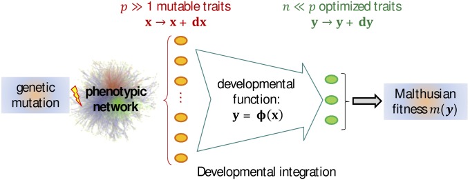
Model of genotype–phenotype–fitness map. This schematic representation shows the different levels of integration assumed in the model, from a single genetic change in the DNA (left) to its effect on the Malthusian fitness of the whole organism. Each mutation pleiotropically affects a large subset of p “mutable traits” (orange ovals), via a complex interaction network among proteins. The parent phenotype at all these traits is represented by the vector x. The effect of a mutation (on the offspring’s phenotype) is a random small perturbation $dx$ with mean zero and arbitrary multivariate distribution (covariance V). These basic mutational changes “percolate” through the network of interactions to induce changes at a much smaller set of n key integrative traits (“optimized traits,” green ovals), which are those under stabilizing selection, represented by the vector y. An arbitrary developmental function $y=\mathbf{\phi }(x)$ relates mutable to optimized traits (developmental integration). The effect of mutations on y is a perturbation vector $dy$ that is approximately linear in $dx$ (to leading order), with linear coefficients $b_{ij}={\partial }_{x_j}\phi (y_i)$, arbitrarily distributed. The optimized traits directly determine fitness via a locally quadratic function $m(y)$ around some optimum (set at $y=0$).

Practical illustrations:

First, let us consider a practical (but limiting) example with a mutation affecting an enzyme involved in metabolism, in a unicellular organism. Mutations at the focal gene modify the concentrations of the products and substrates of the reaction catalyzed by the enzyme and in turn modify many other metabolite concentrations, via the metabolic network. This in turn alters a set of key metabolites (ATP, NADPH, etc.) that directly determine the cellular growth rate via an optimizing function. In the microbial metabolic network models used in flux balance analysis (see, e.g., Price et al. 2004), this optimization function is empirically defined and calibrated. In this example, the concentrations of the p metabolites modified by mutations are the mutable traits (x), and those of the n metabolites determining cellular growth are the optimized traits (y). The metabolic network relating these metabolite concentrations determines the developmental function $\mathbf{\phi }(x)$, and the optimizing function relating the key metabolites to cellular growth is the fitness function $m(y)$.

In metabolic theory, the optimizing function is constructed to define an optimum, but not necessarily with respect to all the factors that enter the function. For example, some metabolite concentrations may enter the function in a linear fashion but be determined by other metabolite concentrations via quadratic functions. In that case, the corresponding optimized traits would be these lower-level metabolite concentrations that do not enter the optimizing function explicitly.

In a recent study, Le Nagard et al. (2011) simulated a phenotype–fitness landscape with underlying phenotypes encoded by a neural network (mimicking a set of interacting genes), which itself determines fitness. This is akin to the type of landscape considered here, and, indeed, the authors analyzed their results using complexity definitions from the FGM. However, their approach differs from ours in that their fitness is a Gaussian function of the distance between a genotype’s reaction norm (to some environmental variable) and some optimal reaction norm. On the contrary, our fitness function depends on distances from a single phenotypic optimum, in fixed conditions.

Existence of a fitness optimum:

To define the set of optimized traits, I assume that there is, at a local scale in phenotype space, a phenotypic state $y=0$ that maximizes fitness. This idea, initially introduced by Fisher (1930) in his geometrical model, is the common ground of many evolutionary models of course, but it is also supported by some observations from long-term evolution experiments (Elena and Lenski 2003). In such experiments, the fitness of replicate populations reaches a plateau [which may sometimes vary (Schoustra et al. 2009)] or at least shows a striking deceleration. Consistent with this finding, negative epistasis among beneficial mutations has been repeatedly reported: beneficial mutations tend to be less advantageous when arising from fitter parents (MacLean et al. 2010; Chou et al. 2011 ; Khan et al. 2011; Sousa et al. 2011). These observations are obviously suggestive of the existence of an optimum for fitness, at some local scale at least.

Local approximation:

Assumptions 2 and 3, respectively, state that the parental phenotype is not too far from the optimum and that mutation effects around this phenotype are mild. These are justified if we accept that, while there may be substantial adaptation going on, a genotype cannot be too far from a local optimum and remain viable. These ideas can be traced back to Fisher (1930) in the presentation of his geometrical model; we use them here to allow several key mathematical approximations.

Under these conditions, the entire population (parent plus mutants) lies in some vicinity of the optimum and will remain so over the course of the adaptive process. This allows a key simplification: we can derive the DFE from only the local behavior of the fitness function $m(y)$ about its optimum $y=0$. This local behavior is simply given by a Taylor-series approximation around the optimum. Assume that, in some local neighborhood, a real function $m:{\mathrm{ℝ}}^n\to \mathrm{ℝ}$ is continuous and defines a “nondegenerate” optimum (one whose second derivative is not vanishing, details below). Then, there always exists a unique set of (Cartesian) coordinates for the y space such that, in the vicinity of the optimum, the function can be written as $m\left(y\right)=m\left(0\right)-1/2\Vert {y\Vert }^2$, where $\Vert {y\Vert }^2={\displaystyle {\sum }_{i=1}^n{y}_i^2}$ is the squared norm of y. The factor $1/2$ is merely for consistency with conventions in the FGM. This statement can be proved in two steps. First, a second-order Taylor-series approximation of any smooth fitness function about a (nondegenerate) optimum yields a quadratic function with positive-definite selective covariance matrix (Lande 1979). Second, one can use a linear transformation of this coordinate system so that the selective covariance matrix in the new system is equal to identity. The particular linear transformation is obtained by solving the generalized eigenvalue problem, (as, e.g., in Martin and Lenormand 2006b; Chevin et al. 2010). Here, the resulting coordinate system has a locally quadratic and isotropic fitness function; namely, all resulting phenotypic directions are equivalently selected. The interested reader can relate this result to the more general “Morse lemma.” Trait definitions are arbitrary in the FGM (Orr 2000; Martin and Lenormand 2006b), so we can choose to define y in those coordinates where, “locally,” the function is isotropic and quadratic. This is possible because we are not focusing on particular traits, as typical quantitative genetics does, so the coordinate system can be arbitrarily “bent” and turned via this linear transformation. Once the coordinate system has been set in this manner, the traits in y are fully and uniquely characterized, contrary to the FGM in its original form. In the following, all other coefficients are defined in this particular set of coordinates.

The assumption that the optimum is “nondegenerate” deserves some development. It means that the function must be twice differentiable, with zero first derivatives at the optimum [${\partial }_{y_i}m\left(\mathbf{0}\right)=0$] and nonzero second derivatives around this optimum [${\partial }_{y_i}^{2}m\left(y\right)<0$, to define a maximum]. Most continuous functions have only nondegenerate critical points (maximum, minimum, or saddle point). However, the approximation cannot be invoked for some special optimization functions that happen to have been used in some previous versions of the FGM. Linear fitness functions of the form $m\left(\mathit{y}\right)=m(\mathbf{0})-\Vert \mathit{y}\Vert$ (Poon and Otto 2000) or fitness functions of the form $m\left(\mathit{y}\right)=\text{exp}(-{\Vert y\Vert }^Q)$ where $Q>2$ (Tenaillon et al. 2007; Gros and Tenaillon 2009) have a “degenerate” optimum at $y=0$. The former function is not differentiable at $y=0$, while the latter has vanishing second derivatives at $y=0$. Note also that even discontinuous functions relating phenotype to growth rate can yield continuous Malthusian fitness functions once some nonheritable and continuous microenvironmental random component is accounted for. Figure 2 illustrates the types of fitness functions where the quadratic approximation does or does not apply. A wide variety of functions are allowed of course, like the Gaussian, asymmetric functions, etc.

Figure 2.

Applicability of the quadratic approximation around the optimum, for various fitness functions. Different fitness functions $m\left(y\right)$ (indicated in inset) are illustrated in one dimension ($y\in \mathrm{ℝ}$). Conditional on the existence of a nonvanishing second derivative at the optimum ($m^{″}\left(0\right)\ne 0$), the quadratic approximation (dashed line) applies (A) or does not apply (B).

The local approximation (“vicinity of the optimum”) allows generalizations but imposes a limit: How close to the optimum must we remain to apply the approximation? As for any Taylor-series argument, the answer depends on the fitness function and cannot be general: the population must remain close enough to apply the approximation.

Pleiotropy within networks:

Assumption 4 requires that the space of mutable traits has high dimension (high pleiotropy, $p\gg 1$): it allows the use of large-number arguments in the statistical treatment of the model. Some a priori and a posteriori arguments suggest that these assumptions are biologically reasonable. Note that I use a particular definition of pleiotropy relating to the whole set of possible mutants in a given genetic target; while some define pleiotropy at the scale of any particular mutation (Wagner and Zhang 2011), these two definitions should coincide if the distribution of mutation effects is continuous.

First, a widely observed feature in most phenotypic networks [from gene regulation to protein interactions or metabolism (Barabasi and Oltvai 2004)] is the “small-world” property. This property implies that every node in the network is connected to most other nodes via a path of short length. We can thus expect that any mutation that affects a given node will in turn modify many other phenotypes through this set of short paths. This suggests that most mutations should be highly pleiotropic ($p\gg 1$, assumption 4). It does not, however, imply “universal pleiotropy”: p can still be substantially smaller than the total number of phenotypes under genetic control (see the discussion in Wagner and Zhang 2011, 2012; Hill and Zhang 2012). Note that this small-world property is a sufficient condition to obtain high pleiotropy, but is not necessary.

Second, this a priori argument is reinforced by a posteriori empirical observations. The metabolome of the actinomycete Nocardiopsis has been shown to be widely modified by resistance mutations caused by single-nucleotide changes (Derewacz et al. 2013): more than 300 different metabolites expressed in the mutants are undetected in the wild type, and up to 80 metabolites in the wild type are undetected in the mutants. Note that mere changes in metabolite concentrations are not counted in this picture. RNA-chip studies have also revealed that the expression of many genes can be jointly altered by simple genetic changes, e.g., gene deletions (Wagner 2002) or single fixed mutations in experimental evolution (reviewed in Hindré et al. 2012).

Developmental integration:

Our last biological assumption 5 requires that the many mutable traits affect a much smaller subset of optimized traits ($n\ll p$). We refer to this assumption as “developmental integration” (although development may not be involved), because it refers to integration through the developmental function, in the sense of Wagner (1984, 1989) and Rice (2002, 2004). It might be the most difficult assumption to evaluate. It is known that oriented networks (like gene regulation networks, for example) are highly hierarchical over several levels, with a few central genes regulating large sets of other genes (Bhardwaj et al. 2010). This hints at integration within biological networks but remains not directly relevant to our model: what is assumed here is that the set of traits (not genes) that determine fitness is small and affected by many underlying traits. More directly, in flux balance analysis (our example above), the function relating metabolism to growth rate has typically a few tens of variables, much fewer than the whole set of metabolites in the system. Also, most of the metabolites in the system affect the key metabolites more or less directly. This assumption is also supported, although indirectly, by the observation that empirical DFEs are not normally distributed. Indeed, if there are many, not fully dependent, phenotypic traits that both mutate and affect fitness (via any function), then the resulting distribution should be close to Gaussian, by the central limit theorem. This is typically not observed: across several organisms, laboratories, and methods, empirical DFEs are skewed toward negative values (reviewed in Martin and Lenormand 2006b; Eyre-Walker and Keightley 2007). Empirical noise could not cause this observation because (i) it is fairly limited in several of these studies and (ii) noise should favor normally distributed observations, which are not observed.

Together, assumptions 4 and 5 are summarized in the notion of high developmental integration: from many traits connected by the network to fewer key traits selected for optimal intermediates ($p\gg n>1$).

Emergence of the FGM

In all of the following, $X.Y$ denotes a matrix product, $X*$ denotes the matrix transposition of X, and $X^{1/2}$ denotes the Cholesky decomposition of X (matrix square root).

Distribution of mutation effects on optimized traits and fitness:

Assumptions 1–4 suffice to obtain a landscape of the type described by an anisotropic Fisher model. Let us see how. From their very definition, mutations create a change in the mutable trait values $dx={\left\{d{x}_j\right\}}_{j\in \left[1,\dots ,p\right]}$, whose multivariate distribution is unspecified (continuous or discrete, etc.). Yet, we require that they have zero mean ($E\left(dx\right)=\mathbf{0}$) and nonzero finite variance–covariance matrix $V=E(dx.dx*)$ and satisfy the Lindeberg and weak dependence conditions (our assumptions 6 and 7). The random perturbation $dx$ translates into $dy={\left\{d{y}_i\right\}}_{i\in \left[1,\mathrm{...},n\right]}$, via the developmental function: $dy=\mathbf{\phi }\left(x+dx\right)-\mathbf{\phi }(x)$. Assumption 3 (mild mutation effects) allows us to take a linear approximation of $\mathbf{\phi }(.)$ about the parent phenotype: $dy\approx B.dx$, where $B={\left\{b_{ij}\right\}}_{i\in \left[1,n\right],j\in \left[1,p\right]}$ is an $n\times p$ matrix containing all the first derivatives of $\mathbf{\phi }(.)$ at the parent position x. We thus retrieve exactly Wagner’s (1984, 1989) linear developmental function, where the $np$ coefficients $b_{ij}$ inB describe how mutable traits $x_j$ integrate into optimized traits $y_i$. I denote them “pathway coefficients,” as they relate to functional pathways connecting phenotypes.

Then, from assumptions 4–7, we can invoke a generalized central limit theorem (CLT). Each $d{y}_i$ is a linear combination of many, not fully correlated, random variables (the $d{x}_j$): under certain conditions on the dependence between $d{x}_j$ and on the nature of their distributions (which may vary across index j), these $d{y}_i$ converge to a normal distribution as p gets large. Assumption 5, not just assumption 4, is required because it implies that the coefficients in B are not zero in a large proportion (p times the proportion of zero coefficients remains large). Assumption 6 applied to the $d{x}_j$ guarantees that the distributions of the $d{x}_j$ pertain to a class that does yield convergence to the CLT as $p\to \mathrm{\infty }$. Technically, the Lindeberg condition is required when the $d{x}_j$ are not all drawn from the same distribution. It is satisfied, e.g., by any distribution whose fourth central moment scales with the squared variance (detailed in theorem 2.35 in Tulino and Verdù 2004) and more generally requires that higher moments be bounded (Baxter et al. 2007). This is an application of the narrower but simpler “Lyapunov condition.” Assumption 7 states that the dependence between the $d{x}_j$ is weak enough that the variance of their mean $V\left(d\overline{x}\right)$ scales with $1/n$ as $n\to \mathrm{\infty }$. It provides one among various sufficient conditions for the CLT to apply with dependent variables (Baxter et al. 2007). The conditions of convergence to the CLT are a vast and well-studied subject of probability theory that is obviously beyond the scope of this article. Our assumptions 6 and 7 thus simply require that we are under those conditions sufficient to apply the CLT, even to dependent and not identically distributed variables. This still encompasses a vast array of situations and distributions.

The CLT then implies that $dy$ converges to a (multivariate) Gaussian as p gets large, with mean $E\left(dy\right)=0$ and covariance matrix $M=E\left(dy.dy*\right)=B.V.B*$, which is denoted $dy \sim N(0,M)$. Note that M may depend on the particular parent phenotype, because both B and V may depend on a position in x space, unless phenotype space for x is additive and the developmental function is linear. I drop the explicit reference to this fact for notational simplicity, but get back to it in the Discussion. Note also that this central limit theorem argument cannot be turned the other way around (from optimized to mutable traits). First, it is the mutable traits that are causally affected by mutation, by definition. Second, the developmental function $\mathbf{\phi }(.):{\mathrm{ℝ}}^p\to {\mathrm{ℝ}}^n$ is not a bijection so we cannot define the inverse relationship $x={\mathbf{\phi }}^{-1}(y)$ that might yield a Gaussian distribution of the $dx$.

Finally, as assumptions 1–3 yield a simple fitness function ($m\left(y\right)\approx m\left(0\right)-1/2 {\Vert y\Vert }^2$), we can express the change in fitness induced by mutations as

$$\begin{array}{l}s\left(dy\text{\hspace{0.17em}|\hspace{0.17em}}y\right)=m\left(y+dy\right)-m\left(y\right)\approx -({\displaystyle \sum _{i=1}^n}{y}_i d{y}_i+\frac{d{y}_i^2}{2}) \hfill \\ dy \sim N(0,M),\hfill \end{array}$$ (1)

for a mutation with effect $dy$ on optimized traits, arising in a parent with phenotype y. In the special case where our fitness component is Malthusian fitness itself, s is exactly the selection coefficient of the mutation. It is also approximately so if $m=\text{log}(W)$, where W is Darwinian fitness with discrete nonoverlapping generations. Otherwise, it describes only a linear change in the measured fitness component. Equation 1 corresponds to an anisotropic FGM (Martin and Lenormand 2006b): the distribution of the phenotypic effects of mutations is Gaussian, and the DFE is a quadratic form in Gaussian vectors, a well-characterized distribution (Mathai and Provost 1992). The difference is that the normality of phenotypic effects emerges from assumptions 3–7 and the central limit theorem, rather than being assumed from the start. Note also that the local approximation for m has reduced anisotropy to the mutational covariance: the selective covariance is $S=I_n$, the $n\times n$ identity matrix (because the fitness function is isotropic).

The DFE in Equation 1 can be expressed in simpler form (see, e.g., Jaschke et al. 2004). Let ${\lambda }_i$ be the n eigenvalues of $M=B.V.B*$, all strictly positive by construction (since V and $B.B*$ are positive definite). Let Q be the eigenbasis of M with column vectors given by the n eigenvectors of M, such that $Q*=Q^{-1}$ and $Q*.M.Q=diag({\lambda }_i)$ is diagonal. Let $z={\left\{z_i\right\}}_{i\in [1,n]}=Q*.y$ be the projection of y in the eigenspace of M (z is simply y expressed in another basis for phenotype space). Finally, let ${\text{χ}}_k^2\left[\nu \right]$ denote a noncentral chi-square deviate with k d.f. and noncentrality parameter ν. The DFE in Equation 1 can be written as a function of a set of independent known random variables (this is called a stochastic representation): we have

$$s\left(dy\text{|}y\right)\mathit{ }\sim \mathit{ }{s}_{\text{o}}-{\displaystyle \sum _{i=1}^n}\frac{{\lambda }_i}{2} {\text{χ}}_1^2\left[\frac{z_i^2}{{\lambda }_i}\right],$$ (2)

where $s_{\text{o}}={\displaystyle {\sum }_{i=1}^n{z}_i^2}/2={\Vert z\Vert }^2/2={\Vert y\Vert }^2/2$ is a constant with ${\Vert z\Vert }^2={\Vert y\Vert }^2$ the distance to the optimum from the parent position (in any orthonormal basis). The DFE is thus fully determined by the parental position in y space and the n eigenvalues ${\lambda }_i$ of M. We thus retrieve a known result from the FGM (e.g., Martin and Lenormand 2006b), in the simpler case where $S.M=M$.

A short comment on what follows is necessary at this point. Because the DFE in Equation 2 depends on the particular set of eigenvalues ${\left\{{\lambda }_i\right\}}_{i\in [1,n]}$, its parameters themselves are random: the ${\lambda }_i$’s are inherently random in our model, as the matrices B and V are random/unknown. The distribution of the eigenvalues ${\lambda }_i$ is called the spectral distribution of M (it is random just as a sample distribution is in statistics). However, we will see that when $n, p\gg 1$, two simplifications occur. First, the DFE is approximately characterized by an expectation over the spectral distribution (the expectation is still random if the distribution is not fixed). Second, the spectral distribution itself proves to converge to a known limit distribution. Together these two points ensure that the DFE is well approximated by a deterministic limit distribution. The following section introduces tools to predict the spectral distribution of M, based only on assumptions 4 and 5 of developmental integration, plus mild mathematical conditions (assumptions 6–8) on the general class of distributions considered; most details are given in File S1.

Spectral distribution of M and random matrix theory

Rationale:

The key principle behind our “statistical treatment” of the model is as follows. It seems impossible to make any a priori statement about the particular values of each pathway coefficient $b_{ij}$ in B or each covariance among mutable traits in V. A way forward is to consider that these coefficients consist of a large set of draws from unknown distributions. Then, as we assume there are many such coefficients ($np\gg 1$), some key properties of the landscape are approximately given by the expected outcome, averaged over coefficients. This is similar to the statistical physics approach and even more closely related to the infinite-allele approximation of quantitative genetics (Kimura 1965). From only distributional, not individual, properties of the microscopic variables, a resulting macroscopic quantity can still be predictable. In our case, the macroscopic variable is the DFE, and the microscopic variables are the underlying phenotypes, their interactions, and mutational properties.

The necessary tool is a description of the properties of the eigenvalues of large random matrices, whose entries are drawn at random following a given scheme. This is a field of probability theory of its own, known as random matrix theory (RMT); see Bai and Silverstein (2010) for a recent review. Our use of RMT here has its equivalent in wireless communication (Tulino and Verdù 2004) or the physics of large nuclei [from which it originates (Forrester et al. 2003)]; the aim is to model some macroscopic properties of a complex system with many elements interacting in a poorly known fashion. The central result from RMT is that the eigenvalues of many large random matrices, once properly scaled, are distributed according to simple predictable limits. As with the central limit theorem (to which RMT is related), these limits are largely independent of the very nature of the distribution of the entries, requiring only the same broad conditions to apply (i.e., assumptions 6 and 7). In addition, it is well established that results from RMT converge quickly (Tulino and Verdù 2004): they already show reasonable accuracy with $n,p$ of the order of 10.

Biologically, these statements imply that, even though the numerous parameters in the model are mostly unspecified (microscopic variables), their collective behavior results in a predictable spectral distribution for M (macroscopic variable); see File S1. This in turn results in a predictable DFE, as detailed in File S2. An obvious advantage is that this asymptotic approximation depends on much fewer parameters than the full model and gets more accurate as the system gets complex (as n and p get large).

Distribution of pathway coefficients:

Let us first characterize the randomness in the entries of matrix $\mathbf{M}=\mathbf{B}.\mathbf{V}\mathbf{.}{\mathbf{B}}^{*}$. Matrix $\mathbf{B}={\left\{b_{ij}\right\}}_{i\in \left[1,n\right],j\in \left[1,p\right]}$ is an $n \times p$ matrix of pathway coefficients: for a given index $i\in [1,n]$, the line vectors of B, denoted ${\mathbf{b}}_i={\left\{b_{ij}\right\}}_{j\in [1,p]}={{\mathbf{\phi }}^{\prime }}_i(\mathbf{x})$ given by the p derivatives, with respect to mutable phenotypes x, of the developmental function ${\mathbf{\phi }}_i(.)$ determining the optimized trait $y_i$. The n vectors ${\mathbf{b}}_i=\{b_{i1},\mathrm{...},b_{ip}\}$ can always be seen as n draws from an unspecified multivariate distribution in ${ℝ}^p$. The $b_i$ have a given $1\times p$ mean vector ${\mathbf{\mu }}_{\mathbf{B}}=E({\mathbf{b}}_i)$ and a given positive definite $p\times p$ covariance matrix ${\mathbf{C}}_{\mathrm{B}}=\mathrm{E}\left(\left({\mathbf{b}}_i-{\mathbf{\mu }}_{\mathbf{B}}\right).{\left({\mathbf{b}}_i-{\mathbf{\mu }}_{\mathbf{B}}\right)}^{*}\right)$.

The nature of the distribution from which the vectors $b_i$ are “drawn” remains fairly general; they must satisfy only the mild mathematical assumptions 6–8. This ensures that central limit arguments may apply (same as discussed for $d{x}_i$) and that we can express the $b_{ij}$ as a linear combination of independently distributed variables $h_{ij}$ (assumption 8). We additionally require that the entries of B do not include a large class at $b_{ij}=0$ (this is implicit in assumption 5 of developmental integration): B is not too “sparse.” The distribution of $b_{ij}$ may vary across index j: the sets ${\left\{b_{i{j}_1}\right\}}_{i\in [1,n]}$ and ${\left\{b_{i{j}_2}\right\}}_{i\in [1,n]}$, with $j_1\ne j_2$, can be drawn from distinct distributions, provided all distributions satisfy the Lindeberg condition (assumption 6, as for the $d{x}_j$ above). As we have seen above for the $d{x}_j$, a narrower sufficient condition is that the fourth moment scale with the square of the variance.

By assuming that $C_B$ is positive definite, we ensure that assumptions 7 and 8 are satisfied: the $b_{ij}$ are not fully correlated across columns j. However, I conjecture (see File S1B) that this entails a somewhat hidden limit: because $n\ll p$ (assumption 5), the pathway coefficients cannot be too correlated among rows i. There cannot be too much similarity between the pathways relating various $x_j$ to each optimized trait $y_i$, because this would imply that $C_B$ becomes positive semidefinite. The effects of such correlations of the $b_{ij}$ among rows i are tackled quickly in the Discussion and File S1B.

Under the broad conditions described above, the matrix $M=B.V.B*$ has the structure of a “sample covariance matrix” (Bai and Silverstein 2010): it is of the form $M=K.K*$, where K has random entries (detailed in File S1B). Note, however, that there is no form of actual “sampling” going on here, of course.

Convergence to a limit spectral distribution:

The key insight from RMT is that the spectral distribution of such a sample covariance matrix $M=K.K*$ is well approximated by a nonrandom (predictable) limit, when the dimensions $(n,p)$ are large. This limit is called the limit spectral distribution (LSD) of M. We can define the spectral distribution of M by its unknown probability density function (pdf) denoted ${\rho }_M\left(x\right),x\in {\mathrm{ℝ}}^{+}$. The corresponding predictable limit when $np\to \mathrm{\infty }$ is the LSD of M, with the pdf denoted ${\tilde{\rho }}_M\left(x\right):{\rho }_M\Rightarrow {\tilde{\rho }}_M$.

The Marchenko–Pastur law for standard sample covariance matrices:

Our results rely heavily on a cornerstone of RMT, known as the Marchenko–Pastur (M-P) law. Mathematical details can be found in Tulino and Verdù (2004) and Bai and Silverstein (2010). Let us consider an $n\times p$ matrix H with “standardized” independent entries, namely with real entries independently drawn from (possibly distinct) distributions with zero mean and variance $1/n$, satisfying the Lindeberg condition (our assumption 6). As $np\to \mathrm{\infty }$ with $p/n=\beta$, the spectral distribution of $H.H*$ converges to the M-P law, its limit spectral distribution. This result is independent of the nature of the parent distribution from which the entries $h_{ij}$ are drawn (uniform, Gaussian, etc.). The M-P law has a simple analytic pdf, which depends only on $\beta =p/n$. The matrix $H.H*$ may be scaled arbitrarily, by some constant ζ, yielding a “scaled M-P law,” with two parameters β and ζ, which I refer to as $\text{MP}(\beta ,\zeta )$. A detailed presentation of this distribution is given in File S1A; I give only its pdf in the case $\beta >1$, which is our focus here:

$$\begin{array}{l}{\rho }_{\zeta H.H*}(x)\Rightarrow {\tilde{\rho }}_{\zeta H.H*}\left(x\right)=\frac{\sqrt{\left(b-x\right)(x-a)} }{2 \pi \zeta x},\hspace{1em}x\in [a,b]\hfill \\ \hspace{1em}a=\zeta {\left(1-\sqrt{\beta }\right)}^2\hspace{1em}\text{and}\hspace{1em}b=\zeta {\left(1+\sqrt{\beta }\right)}^2.\hfill \end{array}$$ (3)

The mean of this distribution is $E\left(\lambda \right)=\zeta \beta$, and its variance is $V\left(\lambda \right)={\zeta }^2\beta \text{.}$ A crucial point is that this distribution is bounded: $\zeta {\left(1-\sqrt{\beta }\right)}^2<\lambda <\zeta {\left(1+\sqrt{\beta }\right)}^2$. This implies that, as β gets large (i.e., when $p\gg n$), all the eigenvalues of $\zeta H.H*$ converge to a constant value $\tilde{\lambda }=\zeta \beta$. This property is the basis of the convergence of the model to the isotropic FGM in the presence of developmental integration (assumptions 4 and 5).

Figure 3 shows the agreement between the spectral distribution of large simulated random matrices (see File S3) and the LSD in Equation 3. Note that these are not means over several simulations; every simulated matrix has spectral distribution approximately given by its LSD. The range of λ narrows as $\beta =p/n$ increases: this can be intuited by considering sampling covariance matrices. The M-P law describes the limit distribution, as $n,p$ get large, of the eigenvalues of the covariance matrix from a sample of p random vectors, drawn from a multivariate distribution in n dimensions, with parent covariance proportional to identity. As p gets large (while n remains finite) the sample covariance converges to the actual covariance of the parent distribution, which is the identity in n dimensions: $H.H*\to E(\lambda )I_n$.

Figure 3.

Convergence of the Marchenko–Pastur law toward isotropy. The pdf $\rho (x)$ of the Marchenko–Pastur (M-P) law is illustrated for a set of values of the shape parameter $\beta =p/n$ (see inset). The matrices are scaled to have $E\left(\lambda \right)=1$ ($\zeta =1/\beta$). The histograms show the spectral distribution of a simulated Wishart matrix ($n=300,\beta =p/n$), and the lines show the limit spectral distribution given by the corresponding Marchenko–Pastur law $\lambda \sim \text{MP}(\beta ,1/\beta )$ (Equation 3). The spectral distribution is well captured by the M-P law and becomes narrower as the ratio index becomes larger ($n\ll p$, high integration).

Note that, from theorem 3.6 on p. 47 in Bai and Silverstein (2010), Equation 3 applies to any distribution of the $h_{ij}$ (with finite mean and variance) if they are drawn from the same distribution, without requiring the Lindeberg condition (our assumption 6). It extends to the case where they are drawn from distinct distributions, under the additional Lindeberg condition; see the details in theorem 3.10 on p. 51 in Bai and Silverstein (2010) and theorem 2.35 on p. 56 in Tulino and Verdù (2004).

File S1A summarizes a set of known results on the M-P law (details can be found in Tulino and Verdù 2004). File S1B applies it to the problem at hand: first, showing that the mutational covariance matrix $M=B.V.B*$ is a sample covariance matrix and then deriving its LSD. In short, M can be equated to $M=K.K*$, where $K=H.W^{1/2}+U_K$ is “linearly” related to a standardized random matrix H. This is ensured by our assumption 8. Matrix H is as described above: an $n\times p$ matrix H with entries independently drawn from (possibly distinct) distributions with zero mean and variance $1/n$. Matrix $W=n{C}_B^{1/2}.V.C_B^{1/2}$ is a positive definite $p\times p$ matrix whose eigenvalues are the same as those of $nV.C_B$ and are finite. Matrix $U_K$ is an $n\times p$ matrix of rank 1, with unique singular value equal to $\theta =\sqrt{{\mu }_B.V.{\mu }_B}$. An approximation for the LSD of M is then obtained as a scaled M-P law.

Results

Approximation to the spectral distribution of M

This section gives an approximation for the LSD of M and then moves toward more simplification, looking for situations where all ${\lambda }_i\approx \tilde{\lambda }$ converge to a single positive constant (convergence to isotropy).

In the absence of developmental or mutational correlations:

A first simple statement is that the M-P law is exactly the LSD of M when $K=H$. This happens whenever the pathway coefficients are unbiased (${\mu }_B=0$) and both mutation effects on x and pathway coefficients are independent with equal variance ($V.C_B\propto I_p$, the identity matrix in p dimensions). Then $M=\zeta H.H*$, where ζ is a scaling constant. Its LSD is the M-P law $\lambda \sim \text{MP}(p/n,\zeta )$, whose pdf is given by Equation 3: ${\rho }_M\left(x\right)\Rightarrow {\tilde{\rho }}_M\left(x\right)={\tilde{\rho }}_{H.H*}(x)$, as $n,p\to \mathrm{\infty }$.

General case with ${\mu }_{\text{B}}=0\mathit{:}$

Let us now consider the more general model, with arbitrary covariance matrices ($V,C_B$), but still assuming that the distribution of pathway coefficients is unbiased, so that ${\mu }_{\text{B}}=\mathbf{0.}$ Then $M=H.W.H*$ ($K=H.W^{1/2}$) and its LSD are no longer an M-P law. Yet, it is shown in File S1B that, with high developmental integration ($n\ll p$), the LSD of M is still approximately an M-P law, with coefficients modified to account for mutational/developmental covariances ($V.C_B\ne I_p$). The impact of these covariances on $\tilde{\rho }(\lambda )$ can be predicted from the sole knowledge of the mean and coefficient of variation of the eigenvalues ${\lambda }_W$ of W. I denote the mean of these eigenvalues $E\left({\lambda }_W\right)={\zeta }_W$ and their coefficient of variation ${\mathit{cv}}_W^2=V({\lambda }_W)/E{\left({\lambda }_W\right)}^2$. The LSD of M is approximately

$$\lambda \sim \text{MP}\left(\frac{p_{\text{e}}}{n},{\zeta }_{\text{e}}\right),\text{\hspace{1em}where }\{\begin{array}{l}{p}_{\text{e}}= \frac{p}{1+{\mathit{cv}}_W^2}\hfill \\ {\zeta }_{\text{e}}={\zeta }_W p/p_{\text{e}}.\hfill \end{array}$$ (4)

The effective parameters $p_{\text{e}}$ and ${\zeta }_{\text{e}}$ account for the effect of multiplication by $W=n C_B^{1/2}.V.C_B^{1/2}$. The phenotypic covariances within the network, both among mutable traits (V) and among pathway coefficients ($C_B$), jointly affect the system but simply by reducing the effective ratio index of the M-P law, by a factor $1/(1+{\mathit{cv}}_W^2)$. The effect ${\mathit{cv}}_W^2$ is the same as that seen in Figure 3 when β becomes smaller: a widening of the spectral distribution, namely an increase in anisotropy among dimensions. Both V and $C_B$ contribute to increase this anisotropy through ${\mathit{cv}}_W^2$.

Full model with arbitrary ${\mu }_B:$

It remains to state how the presence of a bias in the distribution of pathway coefficients $b_{ij}$ affects the LSD of M. This is detailed in File S1B. We have seen that $M=K.K*$, where $K=H.W^{1/2}+U_K$, so the only effect of the bias is to add the rank 1 matrix $U_K$ to the model described by Equation 4. To gain an intuition for the effect of this bias, consider an extreme case. If the entries in $U_K$ are much larger than those in W, then $K\approx U_K$. In this situation, the mutational covariance is driven by the term due to bias ($M=K.K*\approx U_K.U{*}_K$), yielding a covariance matrix of rank 1 (because $U_K$ is of rank 1), namely with a single dominant direction. More precisely, this should happen when $\text{Tr}\left(U_K.U{{*}_K}^{}\right)={\mu }_B.V.{\mu }_B\gg \text{Tr}\left(H.W.H*\right)=\text{Tr}(V.C_B)$, where $\text{Tr}(.)$ stands for matrix trace.

This effect of a small rank in the mutational covariance was described in detail in Chevin et al. (2010). Now the actual situation is less extreme, because M is positive definite, so that all eigenvalues are nonzero. The model must therefore behave in between one in n dimensions and one in one dimension.

A more explicit treatment of the effect of ${\mu }_B$ on the LSD of M is given in File S1B, using a recent result by Benaych-Georges and Nadakuditi (2011). It can be summarized as follows. The bias affects only the leading eigenvalue ${\lambda }_1$, which shows a phase transition behavior determined by the ratio

$${\mathit{cv}}^2=\frac{\mathrm{Tr}(V.C_B)}{\mu {*}_B^{}.V.{\mu }_B}.$$ (5)

This corresponds to our intuition: the effect of bias becomes effective whenever $U_K$ affects K substantially. The parameter cv is akin to a coefficient of variation of the pathway coefficients: when the bias is small relative to the variance in pathway coefficients, $\mu {\mathit{*}}_B^{}.{\mu }_B\ll \mathrm{Tr}(C_B)$ and ${\mathit{cv}}^2\to \mathrm{\infty }$. The phase transition occurs at ${\mathit{cv}}^2=\sqrt{n p_{\text{e}}}$. When $\text{ }{\mathit{cv}}^2>\sqrt{n p_{\text{e}}}$, all eigenvalues fall into the M-P law, so that ${\lambda }_1\to {\left(1+\sqrt{{\beta }_{\text{e}}}\right)}^2{\zeta }_{\text{e}}$ (the upper bound of the M-P law in Equation 4). When $\text{}{\mathit{cv}}^{\text{2}}<\sqrt{n p_{\text{e}}}$, ${\lambda }_1$ rises above the bulk of smaller eigenvalues, which remain under the M-P law. This can be summarized by the relative value of ${\lambda }_1=\text{max}(\lambda )$, over the mean of the bulk ($\tilde{\lambda }=E({\lambda }_{i>1})={\beta }_{\text{e}}{\zeta }_{\text{e}}$). Beyond this phase transition, ${\lambda }_1>\tilde{\lambda }$ and there is a favored direction in the mutant phenotype space (the direction associated with the first eigenvector). The factor of increase of the dominant eigenvalue, $\alpha ={\lambda }_1/\tilde{\lambda }$ satisfies

$$\begin{array}{c}\alpha =\frac{{\lambda }_1}{\tilde{\lambda }}\\ \approx \{\begin{array}{l}\left(1+\frac{n}{{\mathit{cv}}^2}\right)\left(1+\frac{{\mathit{cv}}^2}{p_{\text{e}}}\right){\displaystyle \underset{p_{\text{e}} \to \mathrm{\infty }}{\to }}\left(1+\frac{n}{{\mathit{cv}}^2}\right), {\mathit{cv}}^2<\sqrt{n{p}_{\text{e}}}\hfill \\ {\left(1+\sqrt{p_{\text{e}}/n}\right)}^{2}n/p_{\text{e}} {\displaystyle \underset{p_{\text{e}} \to \mathrm{\infty }}{\to }}1, {\mathit{cv}}^2>\sqrt{n{p}_{\text{e}}}.\hfill \end{array}\end{array}$$ (6)

Putting all these results together yields the following spectral distribution for M in the general case:

$$\begin{array}{l}{\lambda }_i \sim \text{MP}\left(\frac{p_{\text{e}}}{n},{\zeta }_{\text{e}}\right) i\in \left[2,n\right]\hfill \\ {\lambda }_1=\frac{\alpha {\zeta }_{\text{e}} p_{\text{e}}}{n}, \hfill \end{array}$$ (7)

where the effective parameters $p_{\text{e}}$ and ${\zeta }_{\text{e}}$ are given by Equation 4 and the factor α is given by Equation 6.

Equations 4–7 are fairly general as they rely on the general results of RMT. They apply for arbitrary distribution(s) of the pathway coefficients, provided they satisfy the (mild) assumptions, 6–8. They also make no assumption on the heterogeneity of the eigenvalues of W, provided it remains finite, so that $p_{\text{e}}$ remains >n in Equation 4 (see File S1B). They do rely on the key assumptions that n and p are large enough to apply these asymptotic limits and that developmental integration is high ($\beta =p/n\gg 1$), namely on assumptions 4 and 5.

Figure 4 shows the accuracy of Equation 7 in approximating the actual spectral distribution of M in different situations. The example uses $n=100$ for visual clarity of the histograms, but the convergence is much quicker, e.g., with n of the order of 10 and p of the order of 100. The general spectral distribution of M is illustrated in Figure 4A, showing that the bulk of the $n-1$ lowest eigenvalues (${\lambda }_{i>1}$) converges to the M-P law approximation, independently of the nature of the distribution of the $b_{ij}$’s and of its mean ${\mu }_B$. For this example, I used a bimodal discrete distribution ($b_{ij}=\pm 1/\sqrt{n}$), a normal ($b_{ij}\sim N\left(0,1/\sqrt{n}\right)$), a uniform ($b_{ij}\sim U\left(-3/\sqrt{n},3/\sqrt{n}\right)$), or a mixture of the latter two (with roughly half of the coefficients drawn from the uniform and the other half into the normal). The corresponding behavior of the dominant eigenvalue ${\lambda }_1$, as a function of cv, is illustrated in Figure 4B. The simulations and figures were generated in File S3. Different distributions of the $b_{ij}$ do not affect the spectral distribution of M, which is always well predicted by the M-P law approximation in Equation 7 (bulk by Equation 4 and ${\lambda }_1$ by Equation 6).

Figure 4.

Spectral distributions under the random phenotypic network model. The observed distribution of eigenvalues of M (spectral distribution) is shown together with the predicted M-P law approximation. In each case, a single random phenotypic network (matrices $H, B$, and V) was drawn and the resulting spectral distribution of $H.W.H*$ is shown. The $n\times p$ matrix of pathway coefficients $B={\left\{b_{ij}\right\}}_{i\in \left[1,n\right],j\in [1,p]}$ was set to have mean vector ${\mu }_B={\left\{{\mu }_j\right\}}_{j\in [1,p]}$ drawn randomly with ${\mu }_j~N(0,\sigma )$ and $p\times p$ covariance matrix $C_B$. The pathway coefficients $b_{ij}$ were drawn from various alternative distributions: discrete bimodal $(\pm 1/\sqrt{n})$, normal, uniform, or a mixture of the two. The covariance matrices $C_B \text{and} V$ were drawn independently as Wishart deviates: $V,C_B~W_{p+1}({\Lambda }_p)/(p+1)$, where ${\Lambda }_p$ is a diagonal matrix. The matrix ${\Lambda }_p$ has p gamma-distributed diagonal entries, thus allowing us to set a high coefficient of variation (${\text{cv}}_W$) (A) of the eigenvalues of W (i.e., of $n C_B.V$). The matrices were scaled so that $E\left({\lambda }_{i\ne 1}\right)=1$ in the bulk and the dimensions were $n=100$ and $p=2000.$ A shows the resulting distribution of the bulk eigenvalues ${\lambda }_{i\ne 1}$ of either $H.H*$ or $H.W.H*$ (see inset) and the corresponding M-P law as solid lines. Each histogram color corresponds to a distinct distribution of the $b_{ij}$. B shows the behavior of the dominant eigenvalue ${\lambda }_1$. The coefficient cv (Equation 5) is set in the simulations via the scaling parameter σ. For each value of cv on the x-axis, the full set of eigenvalues is represented by the circles. Red and blue circles correspond to $b_{ij}$ drawn from normal or uniform distributions (undistinguishable). The range of the bulk (${\lambda }_{i\ne 1}$, orange area) and the dominant eigenvalue ${\lambda }_1$ (green line) are well predicted by the M-P law approximation.

Distribution of fitness effects and isotropic approximations

Isotropic approximation below the phase transition:

Let us assume that ${\mathit{cv}}^2>\sqrt{n p_{\text{e}}}$ (Equation 6), namely that we are below the phase transition where ${\lambda }_1$ rises above the lower eigenvalues. Once the eigenvalue distribution of M is worked out, the DFE is obtained by a relatively straightforward argument, in the limit $\beta \to \mathrm{\infty }$ (high developmental integration). In this case, the effective ratio index must also become large (${\beta }_{\text{e}}=\beta /(1+{\text{cv}}_W^2)\to \mathrm{\infty }$, Equation 4). From the properties of the M-P law (and of the M-P law approximation in Equation 7), all the eigenvalues of M then converge to a single limit: ${\lambda }_i\to \tilde{\lambda }={\zeta }_{\text{e}}{\beta }_{\text{e}}$ (see Figure 3). We denote this result the isotropic approximation because it boils down to isotropy in the FGM: all directions in y space become equivalent. This isotropic approximation is detailed in File S2. Note that, although framed as a simplistic and extreme limit here, this approximation involves more mathematical subtleties than meet the eye. The key quantity to describe the DFE as a function of the LSD of M happens to be robust to substantial variation across ${\lambda }_i;$ this key technical point is illustrated in Figure S1. This is why the simplistic isotropic approximation ends up being accurate in situations where anisotropy is in fact substantial.

In the limit of $p/n\to \mathrm{\infty }$, the isotropic approximation is equivalent to replacing ${\lambda }_i=\tilde{\lambda }$ for all i: recalling that $s_{\text{o}}={\Vert \mathit{y}\Vert }^2/2$, the stochastic representation in Equation 2 then reduces to

$$s \sim s_{\text{o}}-\frac{\tilde{\lambda }}{2} {\chi }_n^2\left[\frac{2s_{\text{o}}}{\tilde{\lambda }}\right], {\mathit{cv}}^2>\sqrt{n p_{\text{e}}},$$ (8)

namely a constant minus a noncentral chi-square deviate with n d.f. and noncentrality $2s_{\text{o}}/\tilde{\lambda }$. This distribution has an analytical pdf: letting ${\mathit{f}}_n\left(x,\nu \right)$ denote the pdf of the noncentral chi square with n d.f. and noncentrality ν, the pdf of the DFE in Equation 8 is

$$f_s\left(s,n,\tilde{\lambda },s_{\text{o}}\right)=\frac{2}{\tilde{\lambda }}{f}_n\left(\frac{2\left(s_{\text{o}}-s\right)}{\tilde{\lambda }},\frac{2s_{\text{o}}}{\tilde{\lambda }}\right),{\mathit{cv}}^2>\sqrt{n{p}_{\text{e}}} , s\le s_{\text{o}}.$$ (9)

This distribution depends on just three parameters ($n,\tilde{\lambda },s_{\text{o}}$), which constitutes a striking reduction in the parameterization of the model. Most importantly, there is no directionality effect on the DFE: the mutant selection coefficients have the same distribution, irrespective of the direction to the optimum from the ancestor position. Only the overall distance to the optimum ($s_{\text{o}}=y^2/2$) counts: this is the isotropic model in its exact form. At the optimum ($s_{\text{o}}=0$), this DFE reduces to the negative gamma distribution $s_{*} \sim -\text{Γ}(n/2,\tilde{\lambda })$, where the “*” refers to the fact that this is the DFE at the optimum.

Beyond the phase transition:

When ${\text{cv}}^2<\sqrt{n{p}_{\text{e}}}$ (Equation 6), anisotropy arises because, even with ${\beta }_{\text{e}}\gg 1$, the leading eigenvalue ${\lambda }_1$ can be strikingly higher than the others (see Figure 4B). This generates a favored direction in phenotype space where mutants tend to arise preferentially. However, this anisotropy is still of a relatively simple form, because the $n-1$ lower eigenvalues can still be equated to a constant whenever ${\beta }_{\text{e}}\gg 1.$ We thus retain a form of isotropic approximation. We can then replace ${\lambda }_i=\tilde{\lambda }$ for all $i>1$, while ${\lambda }_1=\alpha \tilde{\lambda }$, and the stochastic representation in Equation 2 becomes

$$s \sim s_{\text{o}}-\frac{\tilde{\lambda }}{2}\left({\chi }_{n-1}^2\left(\frac{2s_{n-1}}{\tilde{\lambda }}\right)+\alpha {\chi }_1^2\left(\frac{2s_1}{\alpha \tilde{\lambda }}\right)\right),$$ (10)

where $s_{n-1}={\displaystyle {\sum }_{i=2}^n{z}_i^2}/2$ and $s_1=z_1^2/2.$ It is easily checked that, below the phase transition ($\alpha =1$), we retrieve our previous result (Equation 8), by properties of the noncentral chi-square distribution [${\chi }_{n-1}^2\left(a\right)+{\chi }_1^2\left(b\right)\sim {\chi }_n^2(a+b)$ for any $a,b>0$]. The two quantities $s_1$ and $s_n$ depend on the parental position (y or z) relative to the optimum, not just on its distance $s_{\text{o}}$. They sum up to the total maladaptation: $s_{n-1}+s_1={\displaystyle {\sum }_{i=1}^n{z}_i^2}/2=s_{\text{o}}$. They are the contributions to maladaptation of the projections of the parental phenotype (y) onto two orthogonal and complementary phenotypic subspaces: the eigenspace associated with the $n-1$ lowest eigenvalues for $s_{n-1}$ and that associated with the dominant eigenvalue for $s_1$. This time, directionality is introduced: the same overall maladaptation (a given $s_{\text{o}}$) can result in a different DFE, according to the relative contributions of $s_{n-1}$ and $s_1$. Note that, although more complex than Equation 9, this distribution still has only five parameters ($s_{n-1},s_1,\alpha ,n,\tilde{\lambda }$).

Unfortunately, I could not derive a closed-form pdf for this general model, so it would have to be computed as a convolution of two noncentral chi-square pdfs, by numerical integration. A pdf could be derived in the subcase where the ancestor is optimal, so that all mutations are deleterious ($s_{\text{o}}\to 0,s=s_{*}$). The DFE then becomes a sum of two independent negative gamma deviates $s_{*} \sim -\text{Γ}\left((n-1)/2,\tilde{\lambda }\right)-\text{Γ}\left(1/2, \alpha \tilde{\lambda }\right):$ using a result from Di Salvo (2008), its pdf is

$$f{\ast }_s(s,n,\tilde{\lambda },\alpha )=\left(\frac{e^{s/\tilde{\lambda }}{\left(-s/\tilde{\lambda }\right)}^{n/2}}{-s\Gamma \left(n/2\right)}\right){}_{1}F{}_1\left(\frac{1}{2},\frac{n}{2},\frac{-s}{\tilde{\lambda }}\left(1-\frac{1}{\alpha }\right)\right)\frac{1}{\sqrt{\alpha }},$$ (11)

where ₁F₁(.,.,.) is the Kummer confluent hypergeometric function. The left-hand factor in Equation 11 is the pdf of the negative gamma distribution $-\text{Γ}(n/2,\tilde{\lambda })$, which is the DFE when $\alpha =1$ and $s_{\text{o}}=0.$ Consistently, the right-hand term in Equation 11 (hypergeometric function factor) simplifies to 1 when $\alpha =1.$

Figure 5 shows the effect of the phase transition and the agreement between theory and exact simulations of the DFE with randomly drawn parameters (pathway coefficients $b_{ij}$, mutational covariance V, and mutation effects dx). The simulations and Figure 5 were generated in File S3, which can be used to generate similar figures and checks at will. The agreement between Equations 9–11 and the simulated DFEs is good, whether close to or far from the optimum, and both beyond and below the phase transition (Figure 5, B–D). As expected (Equation 4 and File S1), heterogeneity in the eigenvalues of W, which is strong in this example (${{\text{cv}}_W}^2\approx 2$), does not affect the agreement with theory, as long as $p\gg 1.$ Figure 5, B–D, also shows the fast convergence to the asymptotic result, as $n,p\to \mathrm{\infty }:$ here $n=6$ and $p=200.$ Figure 5B illustrates visually the form of anisotropy that is generated by the phase transition for α: a single favored direction emerges, and the model converges more and more to that in one dimension as α gets larger, as suggested by our initial intuition. The consequence for the DFE is shown in Figure 5D.

Figure 5.

Simulated DFE vs. isotropic approximation(s). The distribution of selection coefficients among random mutations is represented for different situations (see File S3). The network was simulated as in Figure 4. The bias μ_B${\mu }_B$ was scaled to obtain a given level of α: $\alpha =1$ (C) or $\alpha =50$ (D). The mutable traits $dx$ were drawn as i.i.d. uniform deviates and scaled to obtain $V\left(dx\right)=V$. Then $dy=B.dx$ was computed and scaled to enforce $E\left(s\right)=-\mathrm{0.01.}$ The n parental coordinates $y_i$ were drawn as standard normal deviates and scaled to enforce a given ${\Vert y\Vert }^2/2=s_{\text{o}}$. The fitness effect of mutations was then computed from y and $dy$ according to Equation 1. All other parameters are indicated in the insets: $n=6, p=200.$ A illustrates the distribution of pathway coefficients, scaled by their variance ($b_{ij}/\sqrt{V(b_{ij})}$) for each situation: below the phase transition [$\alpha =1$: all $b_{ij}$ under the same blue histogram $N(0,1)$] or beyond the phase transition ($\alpha =50$: each color gives the $b_{ij}$ for a given index j for the three first mutable traits). The corresponding anisotropy in the spectral distribution of M is illustrated in B: ellipsoids are the 95% domain of the mutant phenotypes on the three first optimized traits $y_i$. Beyond the phase transition ($\alpha =50$: purple cloud), there is a favored direction in y space. C and D show the corresponding DFE, below (C) or beyond (D) the phase transition, at the optimum ($s_{\text{o}}=0$, blue), close to it ($s_{\text{o}}=\overline{s}$, red), or farther from it ($s_{\text{o}}=5 \overline{s}$, brown). The lines show the corresponding analytic predictions [Equation 9 (C) or Equations 10 and 11 (D)] (see insets).

File S2 details these approximations and why they prove accurate even though the actual model can be relatively far from isotropic. It also provides approximations for the first moments of the DFE.

Fitting empirical DFEs among random single-nucleotide substitutions

To illustrate how these results can be used, I fitted the observed DFE among random single-nucleotide substitutions introduced into two ribosomal genes of the bacterium S. typhimurium (Lind et al. 2010). In this study, a large set of mutants was created by site-directed mutagenesis, and their selection coefficient in competition (at 1:1 ratio) was estimated with high precision (detection limit $\left|s\right|<{10}^{-3}$). I neglected the measurement error in this analysis, whose goal is merely to evaluate the qualitative agreement between theory and data in one example. I fitted the distribution of s among both synonymous and nonsynonymous mutations, because they showed no significant difference in DFE in this study (Lind et al. 2010). As no beneficial mutations were observed (suggesting $s_{\text{o}}=0$), I fitted Equation 11 to the observed distribution of s by maximum likelihood, using R (R Development Core Team 2007). A first fitting procedure was performed on the scaled values [of $s/E(s)$], to find best-fitting values of n and α on scale-free data. Then a full maximization was performed starting with the best-fitting values thus obtained to jointly estimate $(\widehat{\lambda },\widehat{n},\widehat{\alpha })$.

The results of the fits are given in Table 2, and the log-likelihood profiles for the parameters $\widehat{n}$ and $\widehat{\alpha }$ are shown in Figure S3. The resulting fitted distributions are illustrated in Figure 6, showing both the pdf and the cumulative distribution function (cdf). The gamma distribution (Equation 11 with $\alpha =1$) already performs well, a pattern already shown by the original authors (Lind et al. 2010). The two ribosomal genes yield similar estimates for $\widehat{n}$ and $\widehat{\lambda }$. However, in the rpsT gene, a value of $\widehat{\alpha }$ significantly >1 ($\widehat{\alpha }=4.14$) was detected, while no such improvement in fit was obtained by letting $\alpha >1$ for the rplA gene.

Table 2. Fit of the pdf in Equation 11 to empirical distributions of selection coefficients among random single mutations.

Data set	$\widehat{n}$	$\widehat{\alpha }$	$\widehat{\lambda }$	nb par	AIC	$P(\alpha >1)$
Salmonella rplA gene	4.0 [2.7–5.5]	1.20 [1–4.9]	0.0049	3	−408.0	1.0 (NS)
(56 mutants)	3.9	1	0.0052	2	−410.0
Salmonella rpsT gene	5.3 [3.8–7.0]	4.14 [2.2–7.1]	0.0033	3	−473.4	0.025*
(70 mutants)	3.8	1	0.0073	2	−470.4

For each data set the maximum-likelihood estimates (MLE) are given for the fit of a gamma sum model (Equation 11, parameters $n,\tilde{\lambda },\alpha$) and for the pure gamma fit (setting $\alpha =1$). The 95% confidence interval for the value of n is provided (based on a 1.92 point reduction in log-likelihood relative the maximum likelihood). The Akaike information criterion (AIC) and number of fitted parameters (nb par) are given for each model. The P-value [$P(\alpha >1)$] for the significance of the parameter α is given based on a likelihood-ratio test between the pure gamma and the gamma sum models. A Kolmogorov–Smirnov goodness-of-fit test (not shown) does not reject any of the fitted models (but this test is notably too conservative for fitted distributions).

Figure 6.

Fit of the gamma and gamma sum models to empirical DFEs in bacteria. Top, the distribution of selection coefficients among random nucleotide substitutions vs. alternative fitted models: Equation 11 with $\alpha =1$ (a gamma distribution, blue curve) or α freely fitted (a convolution of two gammas, red curve). Bottom, the corresponding empirical cumulative distribution function vs. fitted models. The values of the best-fit parameters are given in Table 2. The significance of the test for $\alpha >1$ vs. $\alpha =1$ is given below the estimated value.

Overall, these results suggest that the prediction proposed here provides a good agreement with empirical DFEs. It is interesting to note that (i) allowing for an extra parameter (α) can sometimes improve the fit relative to the pure gamma and (ii) on the other hand, in the one case where it does so (rpsT), the estimated value was not very high. Telling whether the phase transition ($\alpha >1$) can be ignored or not is of key importance for the predictions on adaptation away from the optimum. This could be done by the type of simple fitting procedure illustrated here.

Discussion

In this article, I sought to build a mathematically tractable phenotype–fitness landscape from a set of qualitative first principles. It relies on five key assumptions about the effect of genetic changes on phenotype and fitness: (1) existence of a fitness optimum, (2) parent not too suboptimal, (3) mutations of mild effects, (4) pleiotropy of mutations on a large set of p phenotypic traits, and (5) high integration from these traits to fewer ($n\ll p$) optimized traits (see Figure 1). A statistical model is then applied to describe a mostly unspecified network of integration from many phenotypic dimensions into fitness. Various laws of large numbers (central limit theorem and random matrix theory) then yield a simplified phenotype–fitness landscape, in the limit of large $np$ and $n\ll p$. This provides explicit results in terms of a few summary parameters. The resulting landscape is well approximated by Fisher’s geometrical model, either in its isotropic form (all directions equivalent, Equations 8 and 9) or with simple anisotropy (one dominant direction plus isotropy in the remaining phenotype space, Equations 10 and 11). The most general result is an approximate stochastic representation for the DFE in the general model (Equation 10), yielding explicit pdfs in two subcases (Equations 9 and 11), as well as the moments of the distribution (File S2). The accuracy of these approximate distributions was confirmed by extensive simulations of various situations (Figure 5 and Figure S2).

Whenever the isotropic approximation is valid, predictions can be made on how the DFE will change with context (environmental or genomic background), based only on fitness measurements. This is the case where empirical tests appear most feasible. Otherwise (with anisotropy), the DFE will be affected by the direction from the parent toward the optimum (not just its distance), which is much more difficult to infer from empirical measures. Assumptions 1–4 alone yield a Fisher model, but isotropy further requires that $n\ll p$ (assumption 5) and that $\alpha \approx 1$ (mild bias in the distribution of pathway coefficients, see Equation 6). In fact, provided $\alpha \approx 1$, isotropy always seems to be a reasonable approximation, even in situations where n is only slightly smaller than p, and, hence, the spectral distribution of M is quite spread (see Figure 4). We propose a tentative justification for this robustness in File S2 and Figure S1.

In what follows, I discuss limitations and several implications of the model for the distribution of mutation fitness effects across genetic or environmental contexts and for parallel evolution.

Model assumptions and limitations

The five central assumptions were presented and discussed in the Methods section, so I do not delve into this here. The two most obvious limitations of the model lie in its local approximations. The first approximation assumes that mutations have mild effects on phenotype (assumption 3), so that the developmental function $\mathbf{\phi }\left(\mathbf{x}\right)=\mathbf{y}$ can be approximated by its linear trend [slope $\mathbf{B}={\mathbf{\phi }}^{\prime }(\mathbf{x})$]. The second local approximation (assumptions 2 and 3) assumes that the parent and its mutants all lie close enough to the optimum that their phenotypes lie below the leading-order quadratic approximation to the fitness function. These assumptions may, of course, break down (strong maladaptation, critical genetic changes that induce large phenotypic changes). Whether the model is robust to strong deviations from these assumptions is a matter of simulating various such deviations, which is beyond the scope of this article (it might be done using File S3). Whether such deviations are actually important in real-life systems is, as for all tests of the model, a matter of generating empirical DFEs, possibly from mutants in particular genes and measured in various contexts (genetic background or environmental conditions). Provided the maladaptation $s_{\text{o}}$ corresponding to these contexts is measured, the model should provide testable predictions. An extension of the model could also consider higher-order approximations to the developmental functions, using tools derived, e.g., by Rice (2004, Chap. 8).

Finally, it was also assumed that mutation effects on mutable traits are unbiased [$E\left(dx\right)=0$]. This potentially limits the generality of the conclusions. The present model yields a gamma distribution (or a sum of two gammas) when the parent is close to optimal. This type of distribution has shown a good fit to empirical DFEs, both in Lind’s data set (Figure 6 and Lind et al. 2010) and in several previous studies (reviewed in Bataillon 2000; Martin and Lenormand 2006b; Eyre-Walker and Keightley 2007). It may thus be reasonable to ignore bias on the $d{x}_j$ in the first approximation. A detailed study of the effects of biased mutation in Fisher’s model can be found in Waxman and Peck (2003, 2004).

Relationship to previous theory

The effect of the phase transition on the DFE (Equation 11) can be related to previous studies on anisotropy and its impact on effective dimensionality $n_{\text{e}}$ (Martin and Lenormand 2006b; Chevin et al. 2010). Below the phase transition, the effective dimensionality (as defined in Martin and Lenormand 2006b) would be close to $n_{\text{e}}=n$, which is consistent with the model being roughly isotropic. Beyond the phase transition and with a large $\alpha \gg 1$, the model would approximately reduce to that in Chevin et al. (2010) with $n_{\text{e}}\approx m=1<n$ and $s_{\text{max}}=s_1$ in their notation. The model is then driven by the mutant effects on the leading direction (eigenspace associated with ${\lambda }_1\gg \tilde{\lambda }$), although the mutational variance is not exactly zero in other directions (because I assumed $p>n$), as was the case in this previous study. The present model can, thus, provide a natural model for parallel evolution, in the same way as that modeled in Chevin et al. (2010), as detailed below. Overall, our statistical approximation of a complex network yields forms of the Fisher model that have already been studied and for which several results have been derived.

Another approximation of the DFE in Fisher’s model, with a parent close to an optimum, has previously been proposed by Martin and Lenormand (2008), who used arguments from extreme-value theory. The present approach follows the same spirit in using a local approximation, but it differs from the extreme value approximation in three respects. First, the latter describes the distribution of only beneficial effects, not deleterious effects. Second, it applies in a potentially narrower range about the optimum, as it requires a low frequency of beneficial mutants, not just a local approximation in phenotype space. Finally, as for all previous work on the Fisher model, Martin and Lenormand (2008) had to assume the normality of mutation effects on optimized traits, whereas here it emerges from more general first principles. The present model can accurately capture fairly high proportions of beneficial mutants (Figure 5, Figure S2).

Finally, the present results might contribute to the debate over pleiotropy and its evolutionary cost (Orr 2000; Wagner and Zhang 2011; Hill and Zhang 2012). In the present model, two unrelated measures of dimensionality are defined at distinct levels of integration (see Figure 1). The dimension of pleiotropy p is the number of not fully dependent traits that are jointly affected by mutations in a given genetic target. It is the quantity often considered in empirical studies of pleiotropy. The second dimension is that of optimization, n, the number of not fully dependent traits that jointly define a local fitness optimum. The two are related by the developmental function $\mathbf{\phi }(.)$. Whenever $n<p$, it is clearly n and not p that affects the DFE and thus has an evolutionary impact: when pleiotropy (p) is higher than the dimension of optimization (n), it is the latter that drives the “cost of complexity.” The recent study by Le Nagard et al. (2011) also appears consistent with our findings. They simulated evolution in a phenotype–fitness landscape where the underlying network of interacting genes could evolve. They showed that complexity, in “Fisherian” terms (roughly our n), could evolve in response to the complexity of the environmental challenge imposed (defined by the complexity of an optimal reaction norm). This evolution was rather independent of the size of the underlying network (which could be a good proxy for p), especially for larger networks (where $n<p$). In this study, too, the cost of complexity seems to be “paid” according to the dimensionality of optimization rather than that of pleiotropy itself.

Relationship to previous empirical findings

A central goal of this study was to propose an explanation for why the Fisher model, with all its simplifications, can still capture some real-life patterns with reasonable accuracy. Simple skewed distributions like the negative gamma have repeatedly shown good agreement with empirical DFEs (reviewed in Bataillon 2000; Martin and Lenormand 2006b; Eyre-Walker and Keightley 2007). This may not be so surprising: with high pleiotropy ($p\gg 1$) and mild mutation effects, we always expect to see such gamma-like DFEs, in permissive conditions ($s_{\text{o}}\approx 0$, see Figure 5). However, an extra parameter arises beyond the phase transition ($\alpha >1$, Equation 11), and adding this parameter improved the fit of the DFE in the rpsT gene in Figure 6. This may also be the case for other data sets where the gamma alone did not capture the fat tail of observed distributions (e.g., Elena et al. 1998), while the tail gets fatter here in Equation 11 as α increases. This result goes beyond optimal conditions: as long as the parent and mutants remain close enough to some local optimum, we expect the isotropic FGM to accurately predict the DFE, with both beneficial and deleterious mutations (Figure 5). This may thus explain why the FGM also provided accurate predictions in several empirical studies of fitness epistasis and/or compensation, in the presence of beneficial mutations (Martin et al. 2007; MacLean et al. 2010; Sousa et al. 2011).

Impact of the genetic or environmental context?

By building a more mechanistic version of the Fisher model, we can evaluate which parameters of the DFE may or may not depend on the context (environment, parental lineage, mutational target). Of course, in the end, this issue can be settled only by empirical testing; in this respect, gene-specific measurements of the DFE (such as in Lind et al. 2010) offer the most promising approach. In its most general form (Equation 10), the model has five parameters ($n,\tilde{\lambda },s_{n-1},s_1,\alpha$). I discuss each of them in turn, assuming a given species, so that variation in the “lineage” context is limited to genetic variation within a species.

Parameter n is the number of traits under optimizing selection (the dimension of optimization, in y space). It might be expected to be fairly stable across contexts within a given species, as it relates to the core internal processes determining fitness. The nature of the traits under selection can also change without affecting the parameter, as long as they remain in roughly the same number. In the empirical example on Salmonella (Figure 6, Table 2), no significant difference in $\widehat{n}$ was detected between mutations within the two genes studied. However, the power to detect such differences was limited, and whether these genes truly pertain to distinct “targets” is difficult to assess: they are part of the same broad class of ribosomal protein genes.

Parameter $\tilde{\lambda }$ summarizes the contribution of mutational covariances on mutable traits (V) and of covariances among pathway coefficients ($C_B$). It may, in principle, be affected by any effect of the context on these covariances. A change in the nature of optimized traits (see above) would also affect $\tilde{\lambda }$, because a different developmental function (from x to y) would then be defined, modifying $C_B$. Yet, because it synthesizes the small contribution from many parameters, it may also prove stable across contexts. Even if V and/or $\mathit{ }{C}_B$ changes across contexts, the resulting effect on the DFE will be negligible if they still average out to the same $\tilde{\lambda }$. Settling this issue could be possible by empirical fitting of the sort described in Figure 6. In Table 2 the estimates of $\tilde{\lambda }$ were fairly similar in the two genes considered. The context here would be the mutational target, which may or may not differ between these genes. More such studies would obviously provide key insights.

Parameter α was the only parameter showing significantly different estimates in the two genes whose DFE was fitted in Figure 6 (see Table 2). This suggests that these two genes did pertain to distinct mutational targets and that α may vary among these targets (in the same environment and genetic background). A simple (maybe too simple) way to account for such a pattern is to consider that each gene “samples” a subset of pathways, with associated coefficients $b_{ij}$, within the larger set of all possible pathways. According to the bias in the $b_{ij}$ sampled by a given gene, ${\mathit{cv}}^2>\sqrt{n p_{\text{e}}}$ or not, and this gene will lie below or beyond the phase transition ($\alpha =1$ or $\alpha >1$, see Equations 5 and 6). This provides a null model to describe genomic variation in the DFE.

Finally, the fitness distance to the optimum [$s_{\text{o}}$ or the pair ($s_1,s_{n-1}$)] is typically expected to vary across contexts. It is the main application of Fisher’s model to summarize the effect of various contexts into variation at a single parameter $s_{\text{o}}$. The genomic background and the environment should jointly determine $s_{\text{o}}$ or ($s_1,s_{n-1}$) a priori. Whether the mutational target (gene) affects these parameters depends on the isotropy of the model. Below the phase transition (Equation 8), all genes “see” the same distance to the optimum $s_{\text{o}}$. Beyond the phase transition, however (Equation 10), the overall distance $s_{\text{o}}=s_1+s_{n-1}$ may be divided into distinct pairs of ($s_1,s_{n-1}$) according to the subspace associated with the leading eigenvalue ${\lambda }_1$ for this gene. This is the basis for potential parallel evolution, by roughly the same process as described in Chevin et al. (2010).

To summarize, the DFE in Equations 8–10 is unaffected by (i) the nature of the distribution of the pathway coefficients or (ii) the nature of the mutation effects on mutable traits, by (iii) their number p (as long as $p\gg n$), or by (iv) their particular values or mutual covariance, as long as they retain the same overall trace $\text{Tr}(V.C_B)$. Overall, the argument above merely shows that several effects of the context should have negligible influence on the DFE, but it does not state that none has an impact. At least one advantage is that all these complex effects can be summarized into the effects of context on five parameters [$n,\lambda ,\overline{s},\alpha ,\text{and} s_{\text{o}} \text{or} (s_1,s_{n-1})$]. All these parameters are measurable empirically, except a priori for the pair ($s_1,s_{n-1}$), which arises when $\alpha >1$ and the parent is suboptimal.

Essential genes

Let us now focus on a particular type of context dependence that has the advantage of having been well studied empirically. In recent years, studies of large sets of gene deletions and their impact on fitness have flourished, mostly in the yeast S. cerevisae. One salient feature that emerged is that genes fall into two distinct categories: “essential” genes (whose deletion is lethal or nearly lethal) and “nonessential” or “dispensable” genes (whose deletion has weak effects). One puzzling finding is that there are essential genes in comparable proportions in most functional gene complexes (Fudala and Korona 2009). Under the model proposed here, there are two simple and testable alternative interpretations for an essential gene. First, if a given gene samples the full set of pathway coefficients, it may by chance sample a set that leads to $\tilde{\lambda }$ larger than usual. This gene would then have higher average effect on fitness, and its deletion might thus be particularly harmful. Alternatively, the gene may sample a set of coefficients with a highly biased distribution (${\mu }_B$ large), so that it falls beyond the phase transition [$\alpha =1+n/{\text{cv}}^2\gg 1$, Equations 5 and 6]. It would then also be particularly harmful when deleted, as $\overline{s}=\left(n-1+\alpha \right)\tilde{\lambda }/2.$ This simplistic view has the advantage of being testable, by extensions of the experiments in Lind et al. (2010) or using the more recent high-throughput method EMPIRIC (Hietpas et al. 2011). The test would consist of measuring the gene-specific DFE in a well-adapted parent ($s_{\text{o}}\approx 0$), in essential vs. nonessential genes. In the first case, the DFE at an essential gene should show a higher $\tilde{\lambda }$ than at nonessential genes (a gamma with large scale). In the second case, it should show a larger value of α (a heavier left tail than the gamma). In the future, this type of method might give valuable insights into gene essentiality. There are also more puzzles with lethal mutations in general than “simply” gene essentiality (discussed in Manna et al. 2011).

Parallel evolution and the genomic DFE

A natural follow-up of this argument is that some environments may lead to parallel evolution in those genes that lie beyond the phase transition (one of the mechanisms generating essential genes, see above). Because the model retrieved is close to the form described in Chevin et al. (2010), their framework applies to describe the DFE over the genome and how parallel evolution can arise. We propose that $\alpha \gg 1$ arises in those genes that sample a biased distribution of pathway coefficients. Those are also the ones likely to generate parallel evolution, in the particular environments where the direction to the optimum corresponds to their dominant direction. In these particular environments, selection will then fix mutations preferentially in those genes that (i) are beyond phase transitions and (ii) have the corresponding leading direction. Note that those genes with $\alpha \gg 1$ might not have noticeable influence on the genomic DFE, which is roughly the mean of the gene-specific DFEs (Chevin et al. 2010), unless there are many such genes across the genome. Yet these genes will be overrepresented among those undergoing parallel evolution.

Extensions of the model and further applications of RMT

This model illustrates the potential of RMT as a tool for multivariate evolution studies. This is not new, as several studies (Wagner 1984, 1989; Martin and Lenormand 2006b; Chevin et al. 2010) have already used random covariance matrices to model phenotypic covariances, but this choice was assumed from the start. Here, the random covariance matrix structure emerges from first principles. The approach could be extended, for example, using results on large “random sparse matrices” (Bai and Silverstein 2010, Chap. 7) to model less connected networks with isolated clusters (a large proportion of zeroes in matrix B). This would correspond to a more “modular” network where each mutable trait affects only a small portion of all optimized traits (contrary to our assumption 5).

Another interesting extension could be to follow the effect of correlations of pathway coefficients among optimized traits ($b_{ij}$ correlated both across j and across i). As explained in the Distribution of pathway coefficients section, the model assumptions forbid, de facto, a substantial correlation of $b_{ij}$ across optimized traits (across i) because $C_B$ would become positive semidefinite. In File S1 (Equations A1.16–A1.20), I consider an extension, suggested by Dave McCandlish, to allow for weakly correlated $b_{ij}$ among the rows i, not only the columns j. An approximate treatment can be found, provided that this correlation remains weak. This extension does not change the structure of the model: we retain an M-P law prediction, but with a further reduction of the ratio ${\beta }_{\text{e}}$. This ratio now takes a finite limit, even as $n/p\to 0.$ Let ${\mathit{cv}}_b$ be the coefficient of variation of the eigenvalues of the covariance matrix of the pathway coefficients ($b_{ij}$) among optimized traits (among rows i). The effective dimensionality $n_{\text{e}}$ (Martin and Lenormand 2006b), which was roughly $n_{\text{e}}=n$ in the model without correlations among rows i, now becomes <n, more precisely $n_{\text{e}}\approx n/(1+{\text{cv}}_b^2$). This additional correlation can thus create anisotropy, but, a priori, of smaller order than what is obtained via the phase transition. My (clearly disputable) claim, here, is that these “developmental” correlations across optimized traits should be fairly weak, as the pathway coefficients $b_{ij}$ result from “percolation,” through many intermediate levels of organization, from the mutable traits j to the optimized traits i.

Without going into detailed extensions, these examples show that even more general models could be handled with tools from RMT.

Conclusion

This model of pleiotropic mutation over a phenotypic network (Figure 1) is less phenomenological than the original Fisher’s model. Yet, it remains uninformative on the functional reason why any mutation has a given fitness effect. This is both a weakness and a strength: because the results prove independent of many details of the phenotypic network, they do not provide any information on it either. Focusing on evolutionary predictions, not on phenotypic networks, the fact that the isotropic Fisher model can emerge is good news. Indeed, it means that we may predict the DFE in various contexts, without much knowledge of its underlying functional determinants, a knowledge that is not available for most species of interest, in most environments.

Literature Cited

- Bai Z., Silverstein J. W., 2010. Spectral Analysis of Large Dimensional Random Matrices, Ed. 2. now Publishers Inc., Hanover, MA. [Google Scholar]
- Barabasi A. L., Oltvai Z. N., 2004. Network biology: understanding the cell’s functional organization. Nat. Rev. Genet. 5: 101–113. [DOI] [PubMed] [Google Scholar]
- Barton N. H., Coe J. B., 2009. On the application of statistical physics to evolutionary biology. J. Theor. Biol. 259: 317–324. [DOI] [PubMed] [Google Scholar]
- Bataillon T., 2000. Estimation of spontaneous genome-wide mutation rate parameters: Whither beneficial mutations? Heredity 84: 497–501. [DOI] [PubMed] [Google Scholar]
- Baxter G. J., Blythe R. A., McKane A. J., 2007. Exact solution of the multi-allelic diffusion model. Math. Biosci. 209: 124–170. [DOI] [PubMed] [Google Scholar]
- Benaych-Georges F., Nadakuditi R. R., 2011. The eigenvalues and eigenvectors of finite, low rank perturbations of large random matrices. Adv. Math. 227: 494–521. [Google Scholar]
- Bhardwaj N., Yan K. K., Gerstein M. B., 2010. Analysis of diverse regulatory networks in a hierarchical context shows consistent tendencies for collaboration in the middle levels. Proc. Natl. Acad. Sci. USA 107: 6841–6846. [DOI] [PMC free article] [PubMed] [Google Scholar]
- Chevin L. M., Martin G., Lenormand T., 2010. Fisher’s model and the genomics of adaptation: restricted pleiotropy, heterogenous mutation, and parallel evolution. Evolution 64: 3213–3231. [DOI] [PubMed] [Google Scholar]
- Chou H. H., Chiu H. C., Delaney N. F., Segre D., Marx C. J., 2011. Diminishing returns epistasis among beneficial mutations decelerates adaptation. Science 332: 1190–1192. [DOI] [PMC free article] [PubMed] [Google Scholar]
- Cooper V. S., Lenski R. E., 2000. The population genetics of ecological specialization in evolving Escherichia coli populations. Nature 407: 736–739. [DOI] [PubMed] [Google Scholar]
- Derewacz, D. K., C. R. Goodwin, C. R. McNees, J. A. McLean, and B. O. Bachmann, 2013 Antimicrobial drug resistance affects broad changes in metabolomic phenotype in addition to secondary metabolism. Proc. Natl. Acad. Sci. USA 110: 2336–2341. [DOI] [PMC free article] [PubMed] [Google Scholar]
- Di Salvo F., 2008. A characterization of the distribution of a weighted sum of gamma variables through multiple hypergeometric functions. Integr. Trans. Spec. Funct. 19: 563–575. [Google Scholar]
- Elena S. F., Ekunwe L., Hajela N., Oden S. A., Lenski R. E., 1998. Distribution of fitness effects caused by random insertion mutations in Escherichia coli. Genetica 103: 349–358. [PubMed] [Google Scholar]
- Elena S. F., Lenski R. E., 2003. Evolution experiments with microorganisms: the dynamics and genetic bases of adaptation. Nat. Rev. Genet. 4: 457–469. [DOI] [PubMed] [Google Scholar]
- Eyre-Walker A., Keightley P. D., 2007. The distribution of fitness effects of new mutations. Nat. Rev. Genet. 8: 610–618. [DOI] [PubMed] [Google Scholar]
- Fisher R. A., 1930. The Genetical Theory of Natural Selection. Oxford University Press, Oxford. [Google Scholar]
- Forrester P. J., Snaith N. C., Verbaarschot J. J. M., 2003. Developments in random matrix theory. J. Phys. A Math. Gen. 36: R1–R10. [Google Scholar]
- Fudala A., Korona R., 2009. Low frequency of mutations with strongly deleterious but nonlethal fitness effects. Evolution 63: 2164–2171. [DOI] [PubMed] [Google Scholar]
- Gros P. A., Tenaillon O., 2009. Selection for chaperone-like mediated genetic robustness at low mutation rate: impact of drift, epistasis and complexity. Genetics 182: 555–564. [DOI] [PMC free article] [PubMed] [Google Scholar]
- Hietpas R. T., Jensen J. D., Bolon D. N. A., 2011. Experimental illumination of a fitness landscape. Proc. Natl. Acad. Sci. USA 108: 7896–7901. [DOI] [PMC free article] [PubMed] [Google Scholar]
- Hill W. G., Zhang X. S., 2012. Assessing pleiotropy and its evolutionary consequences: pleiotropy is not necessarily limited, nor need it hinder the evolution of complexity. Nat. Rev. Genet. 13: 296. [DOI] [PubMed] [Google Scholar]
- Hindré T., Knibbe C., Beslon G., Schneider D., 2012. New insights into bacterial adaptation through in vivo and in silico experimental evolution. Nat. Rev. Microbiol. 10: 352–365. [DOI] [PubMed] [Google Scholar]
- Ibarra R. U., Edwards J. S., Palsson B. O., 2002. Escherichia coli K-12 undergoes adaptive evolution to achieve in silico predicted optimal growth. Nature 420: 186–189. [DOI] [PubMed] [Google Scholar]
- Jaschke S., Kluppelberg C., Lindner A., 2004. Asymptotic behavior of tails and quantiles of quadratic forms of Gaussian vectors. J. Multivariate Anal. 88: 252–273. [Google Scholar]
- Khan A. I., Dinh D. M., Schneider D., Lenski R. E., Cooper T. F., 2011. Negative epistasis between beneficial mutations in an evolving bacterial population. Science 332: 1193–1196. [DOI] [PubMed] [Google Scholar]
- Kimura M., 1965. A stochastic model concerning maintenance of genetic variability in quantitative characters. Proc. Natl. Acad. Sci. USA 54: 731–736. [DOI] [PMC free article] [PubMed] [Google Scholar]
- Lande R., 1979. Quantitative genetic analysis of multivariate evolution, applied to brain:body size allometry. Evolution 33: 402–416. [DOI] [PubMed] [Google Scholar]
- Le Nagard H., Chao L., Tenaillon O., 2011. The emergence of complexity and restricted pleiotropy in adapting networks. BMC Evol. Biol. 11: 326. [DOI] [PMC free article] [PubMed] [Google Scholar]
- Lind P. A., Berg O. G., Andersson D. I., 2010. Mutational robustness of ribosomal protein genes. Science 330: 825–827. [DOI] [PubMed] [Google Scholar]
- MacLean R. C., Perron G. G., Gardner A., 2010. Diminishing returns from beneficial mutations and pervasive epistasis shape the fitness landscape for rifampicin resistance in Pseudomonas aeruginosa. Genetics 186: 1345–1354. [DOI] [PMC free article] [PubMed] [Google Scholar]
- Manna F., Martin G., Lenormand T., 2011. Fitness landscapes: an alternative theory for the dominance of mutation. Genetics 189: 923–937. [DOI] [PMC free article] [PubMed] [Google Scholar]
- Martin G., Elena S. F., Lenormand T., 2007. Distributions of epistasis in microbes fit predictions from a fitness landscape model. Nat. Genet. 39: 555–560. [DOI] [PubMed] [Google Scholar]
- Martin G., Lenormand L., 2008. The distribution of beneficial and fixed mutation effects close to an optimum. Genetics 179: 907–916. [DOI] [PMC free article] [PubMed] [Google Scholar]
- Martin G., Lenormand T., 2006a The fitness effect of mutations in stressful environments: a survey in the light of fitness landscape models. Evolution 60: 2413–2427. [PubMed] [Google Scholar]
- Martin G., Lenormand T., 2006b A general multivariate extension of Fisher’s geometrical model and the distribution of mutation fitness effects across species. Evolution 60: 893–907. [PubMed] [Google Scholar]
- Mathai A. M., Provost S. B., 1992. Quadratic Forms in Random Variables. Marcel Dekker, New York. [Google Scholar]
- Orr H. A., 2000. Adaptation and the cost of complexity. Evolution 54: 13–20. [DOI] [PubMed] [Google Scholar]
- Orr H. A., 2005. The genetic theory of adaptation: a brief history. Nat. Rev. Genet. 6: 119–127. [DOI] [PubMed] [Google Scholar]
- Papp B., Notebaart R. A., Pal C., 2011. Systems-biology approaches for predicting genomic evolution. Nat. Rev. Genet. 12: 591–602. [DOI] [PubMed] [Google Scholar]
- Papp B., Pal C., Hurst L. D., 2004. Metabolic network analysis of the causes and evolution of enzyme dispensability in yeast. Nature 429: 661–664. [DOI] [PubMed] [Google Scholar]
- Perfeito L., Ghozzi S., Berg J., Schnetz K., Lässig M., 2011. Nonlinear fitness landscape of a molecular pathway. PLoS Genet. 7: e1002160. [DOI] [PMC free article] [PubMed] [Google Scholar]
- Poon A., Otto S. P., 2000. Compensating for our load of mutations: freezing the meltdown of small populations. Evolution 54: 1467–1479. [DOI] [PubMed] [Google Scholar]
- Price N. D., Reed J. L., Palsson B. O., 2004. Genome-scale models of microbial cells: evaluating the consequences of constraints. Nat. Rev. Microbiol. 2: 886–897. [DOI] [PubMed] [Google Scholar]
- R Development Core Team, 2013 R: A Language and Environment for Statistical Computing. R Foundation for Statistical Computing, Vienna, Austria.
- Rice S. H., 2004. Evolutionary Theory: Mathematical and Conceptual Foundations. Sinauer Associates, Sunderland, MA. [Google Scholar]
- Rice W. R., 2002. Experimental tests of the adaptive significance of sexual recombination. Nat. Rev. Genet. 3: 241–251. [DOI] [PubMed] [Google Scholar]
- Salazar-Ciudad I., Jernvall J., 2010. A computational model of teeth and the developmental origins of morphological variation. Nature 464: 583–586. [DOI] [PubMed] [Google Scholar]
- Salazar-Ciudad I., Marin-Riera M., 2013. Adaptive dynamics under development-based genotype-phenotype maps. Nature 497: 361–364. [DOI] [PubMed] [Google Scholar]
- Schoustra S. E., Bataillon T., Gifford D. R., Kassen R., 2009. The properties of adaptive walks in evolving populations of fungus. PLoS Biol. 7: e1000250. [DOI] [PMC free article] [PubMed] [Google Scholar]
- Segré D., DeLuna A., Church G. M., Kishony R., 2005. Modular epistasis in yeast metabolism. Nat. Genet. 37: 77–83. [DOI] [PubMed] [Google Scholar]
- Sousa A., Magalhaes S., Gordo I., 2011. Cost of antibiotic resistance and the geometry of adaptation. Mol. Biol. Evol. 29: 1417–1428. [DOI] [PMC free article] [PubMed] [Google Scholar]
- Tenaillon O., Silander O. K., Uzan J., Chao L., 2007. Quantifying organismal complexity using a population genetic approach. PloS ONE 2: e217. [DOI] [PMC free article] [PubMed] [Google Scholar]
- Tulino A. M., Verdù S., 2004. Random Matrix Theory and Wireless Communications. now Publishers Inc., Delft, The Netherlands. [Google Scholar]
- Wagner A., 2002. Estimating coarse gene network structure from large-scale gene perturbation data. Genome Res. 12: 309–315. [DOI] [PMC free article] [PubMed] [Google Scholar]
- Wagner G. P., 1984. On the eigenvalue distribution of genetic and phenotypic dispersion matrices - evidence for a nonrandom organization of quantitative character variation. J. Math. Biol. 21: 77–95. [Google Scholar]
- Wagner G. P., 1989. Multivariate mutation-selection balance with constrained pleiotropic effects. Genetics 122: 223–234. [DOI] [PMC free article] [PubMed] [Google Scholar]
- Wagner G. P., Zhang J. Z., 2011. The pleiotropic structure of the genotype-phenotype map: the evolvability of complex organisms. Nat. Rev. Genet. 12: 204–213. [DOI] [PubMed] [Google Scholar]
- Wagner G. P., Zhang J. Z., 2012. Universal pleiotropy is not a valid null hypothesis: reply to Hill and Zhang. Nat. Rev. Genet. 13: 296. [DOI] [PubMed] [Google Scholar]
- Waxman D., Peck J. R., 2003. The anomalous effects of biased mutation. Genetics 164: 1615–1626. [DOI] [PMC free article] [PubMed] [Google Scholar]
- Waxman D., Peck J. R., 2004. A one locus, biased mutation model and its equivalence to an unbiased model. Biosystems 78: 93–98. [DOI] [PubMed] [Google Scholar]
- Weinreich D. M., Knies J. L., 2013. Fisher’s geometric model of adaptation meets the functional synthesis: data on pairwise epistasis for fitness yields insight into the shape and size of phenotype space. Evolution 67: 2957–2972. [DOI] [PMC free article] [PubMed] [Google Scholar]
- Wolfram Research, 2012 Mathematica Edition: Version 9.0. Wolfram Research, Champaign, IL. [Google Scholar]
Associated Data
This section collects any data citations, data availability statements, or supplementary materials included in this article.