Classification of Dynamical Diffusion States in Single Molecule Tracking Microscopy

Abstract

Single molecule tracking of membrane proteins by fluorescence microscopy is a promising method to investigate dynamic processes in live cells. Translating the trajectories of proteins to biological implications, such as protein interactions, requires the classification of protein motion within the trajectories. Spatial information of protein motion may reveal where the protein interacts with cellular structures, because binding of proteins to such structures often alters their diffusion speed. For dynamic diffusion systems, we provide an analytical framework to determine in which diffusion state a molecule is residing during the course of its trajectory. We compare different methods for the quantification of motion to utilize this framework for the classification of two diffusion states (two populations with different diffusion speed). We found that a gyration quantification method and a Bayesian statistics-based method are the most accurate in diffusion-state classification for realistic experimentally obtained datasets, of which the gyration method is much less computationally demanding. After classification of the diffusion, the lifetime of the states can be determined, and images of the diffusion states can be reconstructed at high resolution. Simulations validate these applications. We apply the classification and its applications to experimental data to demonstrate the potential of this approach to obtain further insights into the dynamics of cell membrane proteins.

Introduction

It remains an elusive dream to be able to follow a protein and its interactions as the protein travels through the cell during its lifespan. Nevertheless, single molecule tracking by fluorescence microscopy allows one to follow a protein in a living cell at high resolution for a short period of time and to record its trajectory (1–6). Tracking of proteins in live cells is a unique approach to obtain details on dynamical protein association and dissociation kinetics in a spatiotemporal manner, and complements other fluorescence microscopy techniques (7–9). Single molecule tracking techniques have given us valuable insight into the dynamics and biological functions of proteins (6,10–12) and the organization of the plasma membrane (13–16). Despite methodological advances and the insight obtained by contemporary analysis methods, there remains a need to further develop analysis tools that can translate experimental data into biological insights. For example, spatiotemporal information on the diffusion of membrane proteins would contribute to a biophysical understanding of the organization of these protein complexes.

Trajectories of proteins obtained by tracking techniques contain information about the interaction and functional states of the protein. For example, the phosphorylation state of many membrane-bound tyrosine kinase receptors is related to the formation of dimers or higher-order aggregates (17,18). Clearly, proteins associated with these aggregates are expected to show lower mobility than free monomeric receptor molecules, which is reflected in their trajectories. Additionally, proteins often transiently interact with other molecules in nanoscale compartmentalization structures in the plasma membrane or with cytoskeletal structures, both resulting in transient slowed diffusion or confinement (4–6,19–23). Not only do interactions with molecules alter protein mobility, but the mobility of a protein also affects the possibility of interactions with other molecules (24–26). A detailed knowledge of the interactions of proteins and their dynamics is therefore important to understand the underlying signal transduction processes and to model the cellular signal regulatory system (24–28).

Translating the trajectories of proteins to biological events, such as protein interactions, requires the classification of protein motion within the trajectories. Protein species transiently exhibit different types of motion. The motion of membrane proteins can often be described by two dynamic populations of pure Brownian diffusion (6,19,23), which we refer to as the diffusion states (Fig. 1 A). It is, however, nontrivial to accurately determine in which diffusion state the protein is residing during the measured trajectory. Several issues hamper faultless state classification. Proteins exhibiting different diffusion states often have overlapping distributions of step sizes (Fig. 1 B). Furthermore, the localization of proteins has a limited accuracy, and the switching between the diffusion states is a stochastic process. Diffusion-state classification methods are needed to determine when, and in what regions, the protein exhibited distinct diffusion behavior. These regions might point toward a role of certain cellular structures in the function of the studied protein species. In addition, the lifetimes of these diffusion states (the inverse kinetic rate) can be directly derived from the diffusion state durations, and are useful parameters to comprehend the role of the studied protein in complexes associated with cellular regulatory systems. The combined insight may eventually reveal the spatiotemporal design principles of cell decision-making (27).

Figure 1.

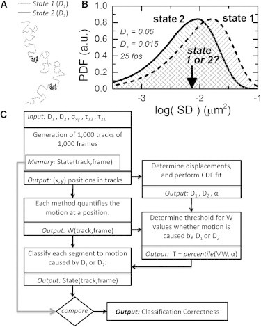
Proposed framework for state classification and problem statement. (A) Schematic to illustrate a typical trajectory of a single protein on a plasma cell membrane, displaying switching behavior between two states with different diffusion coefficients. (B) Distributions of observed squared displacements (SD) resulting from different diffusion coefficients show large overlap. A measured step-size value (an example is indicated with an arrow) cannot be classified with high certainty to unambiguously originate from a particular state, which demonstrates one of the problems to be solved for diffusion state classification. To compose this histogram, a localization inaccuracy σ_xy of 40 nm was added to the positions in the simulations. (C) Scheme of the methodology followed to test the various classification methods on correctness of state classification. After generation of simulated trajectories with dynamic-state allocation, we determine the diffusion constants (D₁ and D₂) and the fraction (α) of the fast state from all displacements using a CDF fit. The track is divided into segments of a certain window length (N), and for each segment the tested quantification methods provide a value W using only the positions in that segment. For each segment the motion is classified as fast or slow diffusion. The threshold (T) for classification is determined from all values W and the fraction α. The center position of the segment is classified as slow diffusion when W is smaller than the threshold T, and as fast diffusion otherwise. The found state is compared with the actual (remembered) state to yield the classification correctness. The same scheme is followed for the diffusion state classification of experimental data. Although the correctness clearly cannot be determined in that case, an estimation of the correctness can be determined by performing simulations at the parameters found by the CDF fit.

A widely used analysis method for single molecule tracking data considers complete trajectories using mean-squared displacement (MSD) curves (3,29–32). For homogenous motion, the shape of the MSD curve contains information about the nature of the diffusion, e.g., pure, confined, or hop diffusion (3,13,33,34). Because the MSD curve is composed of averages of all distances, transient diffusion states cannot be resolved by these full-trajectory MSD analyses (see Fig. S1 in the Supporting Material). When it was realized that protein motion is not homogeneous, but shows transient effects (1,4,10,22,35), local methods were developed that considered subtrajectories (segments) of a trajectory (4,34,36,37). These methods are hampered, however, by the limited number of positions within one segment to obtain accurate diffusion coefficients or confinement strengths. An alternative Monte Carlo-based method (38) is particularly useful to find the kinetic rates between well-differentiated diffusion populations. This method finds diffusion coefficients, their fractions, and the switching rates for the whole set of trajectories, but does not spatially resolve the states. Therefore, we propose what we believe to be a new approach that uses a global method (analyzing all trajectories obtained) to determine the different diffusion states of the protein studied, whereas local methods are used to classify short segments of a trajectory to one of the diffusion states found. We compare several local methods to classify parts of trajectories (segments) to a diffusion state.

Proposed scheme for diffusion state classification

For pure diffusion systems, the multiple diffusion states can be accurately determined using a fit of the cumulative distribution function (CDF) of the squared displacements (20). In this article, we assume that the motion of membrane proteins can be described by two states of Brownian diffusion, termed the “fast” and the “slow” population. Whether this assumption is correct can be checked beforehand by looking at the residuals of a fit of the CDF of step sizes in two-population diffusion (detailed later). After obtaining accurate diffusion parameters by this fit, local methods are used only to classify short segments of a trajectory to one of the diffusion states found. Existing local diffusion or confinement detection methods (34,36,37) can be expanded to yield a local quantification measure that can be used for classification. Subsequently, the classification to a diffusion state is based on a threshold for the quantification measures. This threshold is objectively set using the parameters describing the diffusion states (determined by the fit), and the threshold is therefore based on the experimental data. Thereby, we eliminate the subjective manual thresholding of earlier confinement methods to detect transitions between motion states. The need for manual thresholding was earlier mentioned as a disadvantage of using window (segments)-based methods (39).

We emphasize that there is no need to determine local diffusion values of segments, because the CDF fit has already accurately provided the diffusion values present within the trajectories. The segments only need to be classified to one of the diffusion states. The length of the segments should be carefully chosen such that the corresponding duration is shorter than the typical switching time between states, whereas the duration must be long enough to obtain an accurate measure for the classification. We test different local methods and the influence of different segment lengths for diffusion classification using two-state Brownian dynamics simulations (Fig. 1 C), and compare this approach to a recently developed Bayesian method (40).

Existing motion classification schemes

Several schemes have been proposed to differentiate between the supposed motion types of single proteins found in (sub)trajectories, such as directed, confined, and normal diffusion (33,39,41,42). Three of these schemes consider classification of pure diffusion states (40,43,44). Two of these schemes were based on maximum likelihood estimation (MLE). The scheme devised by Ott et al. (44) employs an MLE approach to classify between diffusive states (also included in our comparison), and uses hidden Markov models to find the diffusion coefficients of these states. The other scheme relies on a large number of localizations and a prior defined number of diffusion-state switching occurrences (43). With contemporary fluorescence microscopy techniques, it is still impossible to accurately localize many positions to find the actual state before the protein switches between states. Furthermore, the amount of diffusion-state switching occurrences is not known beforehand, because this switching is a stochastic process. In 2004, another scheme was proposed that used Bayesian statistics (45) to discriminate between slow and fast Brownian motion in a spatiotemporal fashion without prior knowledge (40). This scheme combines information from thousands of short trajectories to identify the number of diffusive states and the state transition rates, and is included in our comparison.

The classification of confined motion, i.e., motion hindered by transient confinement zones, has been discussed elsewhere (3,20,22,38,39). We emphasize that our approach is not in contrast to the idea of transient confinement zones. In fact, whether the slow diffusion state originates from pure Brownian motion, a transient confinement, or an immobilization of the protein, cannot be revealed from the limited number of typically acquired positions, and requires other experimental and analytical methods. Although the transient confinement and slowed diffusion are closely related, confinement is actually defined as pure diffusive motion restricted by boundaries that cannot be crossed. The confinement area should be of reasonable size such that normal diffusion within this area can still occur. There is no consensus yet on the exact type of motion proteins exhibit.

Materials and Methods

Classification scheme

We provide an overview of our approach to test classification of segments to dynamic two-population diffusion states (Fig. 1 C), followed by a more detailed description of the individual steps. To begin, the two diffusion coefficients and their fractional contribution to the trajectories are determined using a CDF fit of the squared displacements (20). Next, we use one of the different local quantification methods, listed in Quantification Measures in the Supporting Material, which assigns a value to each position in the trajectory. All these methods yield a higher value for a higher diffusion speed. Subsequently, thresholding of these values for the classification is done by taking the αth percentile value of all values found (with α the percentage of step sizes fitted to the first population). For example, when the fraction size of fast diffusion is 0.30, we set the threshold value such that 30% of the values are higher than the threshold value. By taking this threshold, we perform the classification objectively, because the fraction percentage is already accurately determined beforehand from the experimental data itself. To compare the different detection methods in this framework, we tested them using simulated trajectories, where we know the actual diffusion state at each position. The final step in testing the framework is a one-to-one comparison of the found state to the actual (simulated) diffusion state, yielding the classification correctness. We define the classification correctness as the percentage of positions that are correctly classified divided by the total number of classified positions. The state lifetimes τ₁ and τ₂ found by the analysis are compared with the actual lifetimes for the most promising method.

Generation of synthetic trajectories

Two-population diffusion trajectories were generated using MATLAB (The MathWorks, Natick, MA) with the GPUMAT toolbox (8). Each set contained 1000 trajectories composed of 1000 frames (positions) in two dimensions with Brownian diffusion steps in between points. The molecule is allowed to change between diffusion states within a trajectory. In more detail, the positions are given by

$$x_{i+1}=x_i+R\cdot \sqrt{2D_j\Delta t},$$ (1)

$$y_{i+1}=y_i+R\cdot \sqrt{2D_j\Delta t},$$ (2)

where i is the frame number, R is a random number from a standard normal distribution, D_j is the diffusion coefficient of the diffusion state j, and Δt is the time between frames (Δt = 40 ms unless otherwise stated). The dynamical switching behavior between the two diffusion states (e.g., j = 1, also called fast, and j = 2, also called slow) is provided by generating subsequent state durations. The duration of the state is determined by taking a random number from an exponential distribution (a Poisson process) with a given characteristic time τ₁ and τ₂. Diffusion states of all steps in the set are stored, to be able to verify the classification method. Each position (x_i, y_i) is given a localization inaccuracy error by adding a random number from a normally distributed pool with standard deviation σ_xy in each dimension. The localization error in the x-plane σ_x is equal to the error in the y-plane σ_y, therefore σ_xy = σ_x = σ_y.

Cumulative distribution function of squared displacements

To find the diffusion constants D₁ and D₂ and the fraction α of the first population, we calculate the cumulative distribution function of squared displacements for the complete set of trajectories (20). Using the complete distribution yields insights into the behavior of the entire population of single molecules, without ensemble averaging effects. As long as there is a large dataset of displacements to build a reliable CDF, it is a straightforward and reliable method to find the global diffusion coefficients and their fractions. For the two-dimensional case, the CDF for the squared displacements (ΔR)², for a time lag τ = n ⋅ Δt, for two diffusion components is given by

$$\text{CDF}\left(\Delta R^2\left(\tau \right)\right)=1-\alpha \cdot \text{exp}\left(-\frac{{\left(\Delta R\right)}^2}{4D_1\tau +2\left({\sigma }_x^2+{\sigma }_y^2\right)}\right)-\left(1-\alpha \right)\cdot \text{exp}\left(-\frac{{\left(\Delta R\right)}^2}{4D_2\tau +2\left({\sigma }_x^2+{\sigma }_y^2\right)}\right),$$ (3)

where α is the fraction corresponding to the motion with diffusion coefficient D₁. To deal with the localization inaccuracy in the exponent, we determine D₁, D₂, and α for the time lags corresponding to one and two frames, and fit the exponential terms:

$$\text{CDF}\left(\Delta R^2\left(1\right)\right)=1-{\alpha }_{\tau =1}\cdot \text{exp}\left(-\frac{{\left(\Delta R\right)}^2}{4{\hat{D}}_{1,\tau =1}}\right)-\left(1-{\alpha }_{\tau =1}\right)\cdot \text{exp}\left(-\frac{{\left(\Delta R\right)}^2}{4{\hat{D}}_{2,\tau =1}}\right),$$ (4)

$$\text{CDF}\left(\Delta R^2\left(2\right)\right)=1-{\alpha }_{\tau =2}\cdot \text{exp}\left(-\frac{{\left(\Delta R\right)}^2}{4\cdot 2{\hat{D}}_{1,\tau =2}}\right)-\left(1-{\alpha }_{\tau =2}\right)\cdot \text{exp}\left(-\frac{{\left(\Delta R\right)}^2}{4\cdot 2{\hat{D}}_{2,\tau =2}}\right),$$ (5)

which yield the uncorrected diffusion coefficients for each time lag, for example,

$${\hat{D}}_{1,\tau =1}=D_{1,\tau =1}+{\sigma }_{xy}^2,$$

because σ_x² + σ_y² = 2σ_xy², and similarly

$$2{\hat{D}}_{1,\tau =2}=2\cdot D_{1,\tau =2}+{\sigma }_{xy}^2.$$

Now the estimated diffusion coefficient for the first (and similarly for the second) population corrected for the localization error is

$$D_1=2{\hat{D}}_{1,\tau =2}-{\hat{D}}_{1,\tau =1}=\left(2D_{1,\tau =2}+{\sigma }_{xy}^2\right)-\left(D_{1,\tau =1}+{\sigma }_{xy}^2\right)=2D_{1,\tau =2}-D_{1,\tau =1}.$$ (6)

For the fraction α we take the average of the values α_τ=1 and α_τ=2. In the simulations, these two values did not differ by more than a few percent. We have used linear least squares to fit the CDF to the data. Fig. S11 shows an example of a CDF fit for motion with two clearly separated diffusion populations.

Quantification measures

The next step is to quantify the motion of a molecule for each frame in its trajectory. To this end, the trajectories are split in small segments, containing a total number of N subsequent positions (the segment length), and these segments are given a value W by one of the tested quantification measures. Many methods could serve as a measure for slow or fast diffusion. This measure can be, but is not limited to, an estimated diffusion coefficient or confinement index. We have tested the following methods: windowed MSD (34), relative confinement (35,36), the gyration radius (37), and MLE. Besides these windowed measures, we also tested a Bayesian statistics approach (40) using software made available by these authors. A detailed discussion of the measures used can be found in Quantification Measures in the Supporting Material.

State classification

When the motion within a segment is quantified, it can be classified as State 1 (corresponding to fast diffusion with coefficient D₁) or as State 2 (corresponding to slow diffusion with coefficient D₂). We allocate the classification of the segment to the center position of that segment, so that a state duration can still be shorter than the segment length. For the MLE, the classification is performed intrinsically. For the relative confinement and gyration radius methods, the classification is provided by comparing the value W to a threshold value T. A segment is classified as State 1 if W is larger than a threshold value T, and as State 2 otherwise. The threshold value T is determined by taking all found values W, and calculating the αth percentile of these values (with α the percentage of step sizes fitted to the first population). Hence, the already known fraction of the diffusion population is used to define the threshold value for the measure to perform the classification.

In the case of the windowed MSD, we slightly altered the way to determine the threshold T, due to reasons described in the Results. We used a likelihood approach to calculate the chance that a single value W (calculated for a segment) originates from diffusion with D₁ or originates from diffusion with D₂. In more detail, a probability density function (PDF) of W is composed for each diffusion constant given the values of the diffusion coefficients D₁ and D₂. Examples of such PDFs are shown in Fig. S12 A. The threshold value T is chosen as that value of W where the PDF of W from D₁ intersects the PDF of W from D₂ (such that L₁(T) = L₂(T)). In this way, the segment is classified to the most likely state.

The PDF of W for the windowed MSD method for a given diffusion coefficient is calculated as follows: Using a one-population Brownian simulation, a trajectory (containing 10⁶ positions) is calculated. From this, we calculated the values W for all segments in the trajectory. Next, the PDF of the found values W is composed. This procedure is performed for both D₁ and D₂. Finally, the intersection of these two PDFs is determined.

Visualization

After the state classification has been performed, either in simulations or in experimental data, the information obtained can be used for subsequent analysis such as visualization. All the positions of all the molecules in one video recording are used to reconstruct an image, such that one can visualize the areas where the molecules have traveled. Each individual position (localization) is represented by a color-coded dot. The color of the dot depends on the state found at that position and time: red for the slow state, and green for the fast state. This results in diffusion-state images at high resolution showing the areas of slow and fast diffusion. We removed immobile trajectories because these were typically found on the glass substrate and not in cells. The filter for immobile trajectories was based on the gyration method applied on a complete trajectory, with the threshold for the reached area defined by a gyration radius of 40 nm, as this corresponded to the apparent area traveled by an immobile molecule due to the localization accuracy. This means that only those molecules are displayed that exhibit motion at least once.

Live cell experiments

See Live Cell Experiments Methodology in the Supporting Material.

Results

Performance of different quantification measures

We validated our approach by simulating the extreme case of well-separated diffusion constants with D₁ = 40 × D₂ and long-state durations. We obtained a correctness of >95% for windowed MSD, and >99% for the other methods, as expected for clearly distinct motion. Next, we tested the different quantification measure methods for diffusion classification, and studied the influence of different segment lengths therein. Therefore, we simulated (at 25 fps) four cases with two diffusion states with different state lifetimes and localization accuracy. The cases were chosen to provide a challenging and realistic situation for discrimination of the two diffusion constants from experimentally obtained single molecule trajectories.

The diffusion constants were chosen to reflect relatively slow membrane receptors (unpublished observations): D₁ = 0.06 μm²/s, and D₂ = 0.015 μm²/s. (For other ratios of diffusion coefficients, see Fig. S4.) We chose our switching settings close to the values found for the epidermal growth factor (EGF) receptor (4): τ = 300–900 ms. The localization accuracy depends on the number of photons recorded from a molecule per frame. The chosen localization accuracies are typical values observed for quantum dot labels (σ_xy = 20 nm) or fluorescent protein labels (σ_xy = 40 nm), whereas organic dyes will often be somewhere in between these values. The accuracy does not only depend on the number of photons acquired for localization, but also on the labeling strategy. For instance, antibodies are large macromolecules and their flexibility leads to a lower localization accuracy.

Fig. 2 shows the performance of diffusion-state classification for different quantification measures of local diffusion together with the influence of the segment length chosen. For the windowed MSD method, we display the correctness when using the first three points of the MSD curve in the fit, because this gave the best correctness in all the simulation cases. For the first simulation (case A), we chose the localization accuracy σ_xy = 40 nm and the state lifetimes were both set to 300 ms. To study the influence of the localization accuracy σ_xy alone, in simulation case B this parameter was lowered to 20 nm. In simulation cases C and D, only the switching behavior was altered compared to case A to be able to test the influence of the state lifetimes. When the two lifetimes are not equal (case C), this clearly changes the diffusion fractions, such that there are an unequal number of molecules in each state on average. The two diffusion coefficients and their fractions were not assumed to be known beforehand, analogous to experimental data. These state parameters are found for each simulation by a fit to the CDF of squared displacements. The results show that an optimal choice of the segment length is needed to yield the best classification correctness. The optimal segment length depends to a large extent on the state lifetimes and also on the particular quantification measure used in the state classification.

Figure 2.

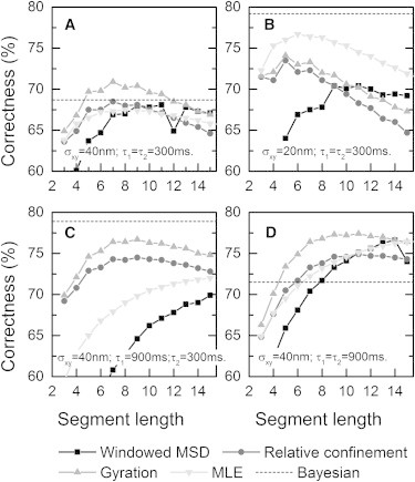
Correctness of the two-population classification by different quantification measures for different simulated cases (A–D in the corresponding panels). The correctness of the different quantification measures is plotted against the segment lengths used in the classification. The Bayesian method does not use segments, and its result is shown (dashed line). In all simulation cases D₁ = 0.06 μm²/s and D₂ = 0.015 μm²/s. (A) Simulation case A has a localization inaccuracy σ_xy of 40 nm and short state lifetimes (τ₁ and τ₂). (B) This simulation case differs from case A only by a lowered localization inaccuracy σ_xy. (C) This simulation case differs from case A only by having a longer fast-state lifetime τ₁. (D) This simulation case also has a longer slow-state lifetime τ₂.

We find that the non-diffusion-based gyration evolution method is the most accurate measure for diffusion-state classification in the simulation cases, with localization accuracy of 40 nm (cases A, C, and D). In these cases, for equally sized diffusion populations (cases A and D), the gyration-based classification scores better than classification using any other method. When the diffusion populations are not equally sized (case C), the gyration-based classification scores almost as well as the computationally much more expensive Bayesian method. In simulation case B with a localization accuracy of 20 nm, the Bayesian method and MLE-based classification score better than the other methods. This trend continues when there is no localization inaccuracy; simulations for this case showed the MLE method then scores 81% correct compared to 74% for the gyration-based classification. In practice, however, the localization will rarely be better than 20 nm, due to the limited number of photons and biochemistry labeling-related issues. In the case of slow-state switching behavior (case D), the gyration-based classification at these state-switching rates is already close to its best possible performance with these diffusion coefficients and localization inaccuracy; increasing the average state duration to infinity only resulted in 3% improvement in correctness. The classification correctness for the windowed MSD achieved when another number of points in the MSD curve is taken to perform the fit can be found in Fig. S2. The classification correctness when we set a minimum state duration for a number of frames can be found in Fig. S3.

After classification of the diffusion inside trajectories, the lifetime of the states can be determined by composing a histogram of state durations and fitting the lifetime. We determined the distribution of the slow- and the fast-state lifetimes found by the gyration-based classification in trajectories of simulation case A (see Fig. S5). We found that the state lifetimes fitted are shorter than the actual (simulated) lifetimes, especially for longer state lifetimes. Additional simulations showed that a trend of changing the state lifetimes in the simulation is reflected in the lifetimes found, although larger lifetimes (as in case D) are significantly underestimated, especially when the correctness is <85%.

Although the correctness percentages provide a measure of the classification performance, the exact number might not give a feeling for how useful such a classification is. We will return to this point in the section on identifying the zones of slow diffusion. Clearly the percentage must be >50% to have any relevance, because this percentage would also be obtained by a completely random state allocation.

Optimized threshold

The windowed MSD, relative confinement, and gyration measures use a threshold for classification. We noticed that for the windowed MSD, the classification correctness was not around its maximum with the threshold at the αth percentile, especially for unequally sized diffusion populations (Fig. 3 A). In the case of simulation case C (i.e., with unequally sized diffusion populations), the best result when using the windowed MSD as the quantification measure would be to classify every position as fast diffusion, and thereby scoring ∼75% correct (i.e., the fast fraction size). However, such classifications would not provide any information. The other methods score the same correctness at the 100th percentile threshold by definition, but these methods score a higher correctness with a threshold at the αth percentile. For the windowed MSD method, we therefore used another threshold. We instead compared the likelihoods that a value W for a segment originates from diffusion with diffusion coefficient D₁ or from diffusion with diffusion coefficient D₂. In other words, the threshold was set at the intersection of the probability density functions of the values obtained with the windowed MSD for diffusion from each diffusion state separately (detailed in Materials and Methods). We verified that the windowed MSD using likelihoods for state classification indeed performed with a higher correctness compared to when window MSD values are compared to a threshold using the αth percentile. Likelihood methods do not regard the fraction size α to determine the most likely state for a segment, therefore the MLE and the Bayesian methods are not included in Fig. 3 A.

Figure 3.

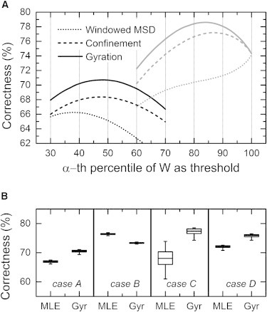
(A) The correctness dependence on the choice of the state classification threshold for simulation case A (left curves) and case C (right curves). The threshold varied with the αth percentile value of calculated quantification-measure values W. In these simulation cases, the fraction size for fast diffusion α = 0.5 and α = 0.75 (cases A and C, respectively), and the classification, was performed with a segment length of seven frames. The windowed MSD method does not yield optimal correctness with a threshold using the αth percentile, yet the optimal threshold does not provide any information either. Therefore the threshold selection for this method was altered to using the likelihood that the found value for a segment corresponds to either of the two diffusion states. (B) Robustness of the MLE and gyration-based classification. When simulations with 100 trajectories and 1000 frames are repeated 100 times, variations can come from the accuracy of the CDF fit. (Box plot) Resulting distribution (5, 25, 50, 75, 95%) of the obtained classification correctness using MLE and the gyration (Gyr) method for all simulation cases (A–D, left to right) due to this effect.

Classification robustness

The values for the classification performance in Fig. 2 and Fig. 3 A are average values that are obtained for many classifications. Because one simulation entailed 1000 trajectories of 1000 frames, the statistical noise averaged out between simulations with the same diffusion parameters. However, analyzing the results of one simulation is not sufficient to predict the robustness of the method, because the robustness in the correctness also depends on other aspects of the classification framework. For example, the correctness depends in large extent on the fitted diffusion constants and fractions obtained from the CDF fit. Therefore, we tested whether small perturbations in the CDF fit influenced the obtained correctness for the MLE and gyration method. We used a segment length of seven frames to classify 100 simulations to obtain the distribution of the correctness. In each simulation we used the simulation settings of case A, except for the number of trajectories in the simulations, which was lowered to 100 trajectories (a realistic number of molecules in a tracking experiment). In this way, fewer displacements are available for the CDF fit, and therefore the fitted values have a larger spread in subsequent simulations. The resulting correctness distributions (Fig. 3 B) shows that neither of the two methods is influenced dramatically by slightly perturbed CDF fits, except for the case where both fractions are not equally distributed (case C). The spread, in that case, is especially large in the MLE method.

Identifying the zones of slow diffusion

After state classification of the diffusion, super-resolution-like images of the diffusion states can be reconstructed. When the distribution of slow diffusion zones is not randomly distributed, the proposed approach for diffusion-state classification should be able to detect these zones. To validate this application, we performed simulations of 200 trajectories where the diffusion state was spatially defined. The regions with slow diffusion were defined as 1 pixel wide (corresponding to 120 nm), and were separated by 5 pixels. The separations were the regions of fast diffusion. The diffusion value in the fast region was chosen D₁ = 0.10 μm²/s, and in the slow regions it was chosen D₂ = 0.01 μm²/s, with the localization accuracy σ_xy = 20 nm. These settings were chosen to represent a typical membrane protein imaged utilizing bright fluorophores. The resulting state lifetimes were ∼300 ms. We performed the diffusion-state classification using the gyration-quantification measure with a segment length of four frames (Fig. 4 and see Movie S1 in the Supporting Material). Simulations with the diffusion-state parameters mentioned showed that this is the optimal segment length. The correctness of gyration-based classification was 85%. The figure shows that the performance is more than adequate to visualize the spatial diffusion-state organization described. The actual states of the simulation and the same reconstruction image using MLE-based classification are shown in Fig. S7. For comparison, when the motion and the state switching is completely random, such as in simulation case A, the reconstruction map also shows apparent zones (see Fig. S6). However, these zones are only caused by the randomness of Brownian movement.

Figure 4.

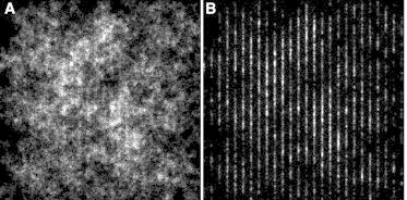
Diffusion states classified by the gyration method, visualized at high-resolution, with images displaying the regions in the fast state (A) and slow state (B). The simulation was designed with spatially defined zones (vertical lines) for diffusion states. Here the slow-state regions were 120-nm wide and are separated by 600-nm-wide fast-state regions. The regions of the slow diffusion state are suitably classified and clearly visible. The dimension of the image is 15 × 15 μm, and the image is reconstructed at a resolution of 30 nm/pixel.

Example of classification applied to EGF receptor

The advantage of spatiotemporal-resolved state classification is the possibility to observe where the molecules have traveled in which diffusion state. Reconstructed videos may also reveal whether multiple diffusion populations are originating from a pool of molecules exhibiting either diffusion state, or a pool of molecules transiently making transitions between the states. The lifetimes of the states can be determined as well from the histogram of state durations.

To demonstrate the potential of the application of diffusion-state classification, we performed a gyration-based classification on experimental single molecule tracking data. We recorded fluorescence images of fluorescently labeled EGF receptor in MCF7 cells by utilizing SNAP-tag (see Movie S2). In this video recording we detected, on average, 210 fluorescent molecules per frame (see Fig. S8 D). The localization accuracy in our video is close to 40 nm. The diffusion constants D₁ and D₂ and the fraction size α of the fast state from all displacements are determined using a fit to the CDF of squared displacements (see Fig. S8). We obtained D₁ = 0.112 ± 0.001 μm²/s, and D₂ = 0.008 ± 0.001 μm²/s with α = 0.69 ± 0.03 (the given errors are 5–95% confidence intervals of the fit). Intercellular differences are larger than the errors of fitting the CDF. We used a segment length of seven frames, which performs best according to simulations for the given diffusion parameters (classification correctness of 86%). State lifetimes (or kinetic rates, the inverse lifetime) were obtained by combining the state durations from five recordings of EGF receptor (unliganded) to get enough statistics (see Fig. S9).

After diffusion-state classification, we reconstructed the diffusion-state video (see Movie S3) and diffusion-state images at high resolution (Fig. 5 and see Fig. S10). In these images, we clearly see distinct zones of slowed diffusion. Furthermore, we see cellular structures such as filopodia at the boundaries of the cell, and possibly collapsed filopodial structures on the lower membrane. The presence of EGF receptor in filopodia was expected, because EGF receptor undergoes retrograde transport in filopodia (46,47).

Figure 5.

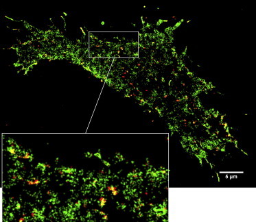
The spatial distribution of the diffusion states exhibited by EGF receptors in an MCF7 cell. The reconstructed image shows the areas where receptors were classified in the fast diffusion state (green), and areas where receptors were classified in the slow diffusion state (red). For a region at the periphery of the cell, a zoomed image (inset) shows clear regions of slow diffusion. The image also shows that the receptor is associated with certain cellular structures such as filopodia. The classification is performed using the gyration method with a segment length of seven frames. The resolution of the reconstructed image is 30 nm/pixel. To see this figure in color, go online.

Discussion

The optimal segment length

The optimal segment length correlated to the state lifetime in our simulations. For example, the optimal seven frames in simulation cases A and B corresponds to the average state lifetime of 300 ms (7.5 frames), and when the state lifetimes increase (simulation cases C and D), the optimal segment length also increases. The optimal segment length also varies for the different quantification measures, especially when the state lifetimes increase (simulation cases C and D). Because the state lifetimes are not known before the classification, it would be preferable when the results do not vary much for different segment lengths. We can see that the gyration method with a segment length of seven frames scores near optimal in almost all the cases simulated. Therefore, a good strategy would be to perform the classification first with the gyration method and a segment length of 5–7 frames. This might provide a good first classification with an adequate correctness. Later, the classification may be repeated with a different segment length more suitable to the state lifetimes found to obtain an optimized classification or a verification of the reconstructed diffusion-state images.

Diffusion state classification

We noticed that the gyration method has higher correctness and is more robust compared to the other tested methods, especially in situations with higher localization errors (σ_xy = 40 nm). The reason may be found in the fact that more information is used to determine the gyration radius compared to the value calculated with the windowed MSD or the MLE methods. In the calculation of the gyration, the information of the distances between all the segments positions is taken into account unlike in MLE. Therefore, the gyration method not only considers the distance between points, but also the relative locations of the positions. For example, for pure diffusion, it is unlikely that a particle would move in only one direction. The MLE would not detect this, because it only considers subsequent distances; however, the gyration method will detect it. The spatial information of relative location of the positions is only considered in the gyration and confinement methods, which might be the reason why these methods scored higher in classification of the two diffusion states. In the windowed MSD method, the optimum result is obtained when the fit to find the diffusion value is obtained from information only up to a time lag of three frames. This means that in the case of the windowed MSD calculation, the distance information from the first to the last point is not considered, whereas this is taken into account in the gyration method. However, when the positions are more precisely known (i.e., low localization error), the MLE and Bayesian-based methods start to outperform the gyration method. An explanation for this might lie in the fact that these methods make use of averaged distances of single steps. The average value of single steps in a segment is apparently precise enough to find the most likely underlying diffusion coefficient. Without localization errors, the (windowed) MSD also scores best when only single steps (corresponding to a time lag of one frame) are considered. Our approach with the windowed MSD is then in fact equivalent to the MLE method (43). Another reason why the windowed MSD scores lower than other methods might be because MSD values can be negative, especially with higher localization errors. It is not clear what the chance is that negative values represent a slow or a fast state (we classified these values as slow), such that negative values cannot be adequately classified.

Interestingly, it remains an open question whether the gyration-based classification method is the optimal quantification measure for the cases simulated, or if another quantification measure can be invented that outperforms gyration-based classification. We saw that classification based on the maximum likelihood of the average of single step sizes is outperformed by gyration-based classification, hence MLE does not yield the optimal performance to this problem. How to best combine all the positional information of a segment remains an open question.

Although we demonstrated the state classification for a two-population system, the framework and the methods can also be used for more than two populations. The CDF fit should then be adjusted for multiple populations, and thresholds can similarly be set at the found αth percentile. This expansion can be benchmarked using simulation situations comparable to those we have presented here. Other quantification methods can also use this framework for benchmarking the method in a realistic context of single molecule experiment on plasma membrane receptors. In this article we have tested prevalent analysis methods for quantification of the local diffusion. Although the confinement and gyration methods have been developed in the context of confinement, they had never been applied for quantification of pure Brownian motion, whereas we showed that these methods outperform classical methods to classify segments to a diffusion state.

Michalet (34) has discussed the practicality of using a windowed MSD. He argued that the segment length must be chosen small enough so as to measure local behavior and not averaged global behavior, yet must still be large enough to be sufficiently accurate inasmuch as too-small windows have a broad distribution in output values. He therefore concluded that this method can rarely provide reliable estimates of the diffusion coefficients, and can only show a difference in multiple orders of magnitude, even for windows of 100 points. Although this conclusion is valid in the case of exceedingly low diffusion coefficients, such as D = 10⁻⁴ μm²/s in his example, we showed that a windowed MSD can still be useful in diffusion-state classification. However, it is indeed not as powerful as the other methods tested.

We chose to use the CDF-fit approach to find the global diffusion values. Another approach to obtain the diffusion coefficients has been described using Bayesian statistics (45) and a hidden Markov model. This method finds the different (and hidden number of) diffusion states with their diffusion coefficients (40). Although this method yields accurate results, it also requires about a thousandfold more computational time on our computer, whereas a CDF fit is comparably accurate. Concerning the accuracy of the quantification measure, we neglected the influence of the exposure time on these values. Whereas this leads to underestimation of the value of the diffusion coefficient due to the averaging blur during exposure (1,48), we only used the values to classify states; the exposure time effect should not have much influence on this classification.

We only regarded spatiotemporal analysis methods in this article, because the spatial information may yield especially important information, such as where a molecule is interacting. Therefore, we have excluded image correlation spectroscopy methods (such as particle image correlation spectroscopy (49,50)) that do not require tracking, and a Monte Carlo approach (38). Also, we only looked at alternating diffusion states, and not at active transport or confinement, as explained before.

Application in live cells

The application of the gyration-based diffusion-state classification approach demonstrated that the correctness achieved is sufficient to identify spatial zones of slowed diffusion within cellular structures. Such zones are particularly important because they reflect the regions where the protein interacts with other proteins or cellular compounds. The physiological meaning of the slow diffusion zones in our example of EGF receptor remains an open question at the moment. They could be related to cytoskeletal structures or regions where the receptor exhibits internalization. For other proteins, we might find another distribution of membrane patches of slowed diffusion, and specific diffusion states near other cellular structures such as actin or microtubuli might be seen. In that case, single molecule trajectories may indicate a role of such cellular structures in the signaling of the protein studied when analyzed by diffusion-state classification.

Diffusion-state lifetimes obtained by this classification framework seem less informative, as they tend to be underestimated due to short periods of incorrect state classification (see Fig. S5). To reliably obtain changes in state lifetimes, a high classification correctness (>85%) seems essential. However, state lifetimes can be used as a test to confirm that the diffusive populations found (using the CDF fit) are lasting longer than the timescale of the sampling rate (time between frames). States with extremely short lifetimes are probably caused by issues with multiple intermixed diffusive states, and further diffusion classification is unreliable in that case.

Conclusion

In summary, we have introduced what we believe is a new strategy for spatiotemporal classification of two-population diffusion, and compared methods to be used for this classification. We have validated our proposed diffusion-state classification approach by testing with simulations and showed possible applications, such as determining diffusion-state lifetimes and composing diffusion-state images. The key feature of the proposed framework is that a diffusion estimator is the logical choice but not necessarily the best way to discriminate and classify segments to two diffusion states. When we have determined the diffusion coefficients and their fractions present in the motion of all the molecules (e.g., using a CDF fit of the squared displacements (20)), there is no need to find a local diffusion coefficient. What remains is the need to classify the local motion to one of the found diffusion states. The found fraction size α can be used to perform objective thresholding of the local quantification measures. This avoids relying on subjective manual thresholding in segment-based methods to detect transitions between motion patterns (39), such as relative confinement (4,36).

We have found that the gyration method is best used for diffusion-state classification when the localization error (due to photon shot noise and the finite proximity of the fluorescent dye to the protein) is ∼40 nm, whereas MLE or Bayesian methods are preferred in the case of localization errors of 20 nm or less. Although the differences in the resulting classification correctness are small, the robustness of the gyration method is higher than the MLE method, especially when a limited number of displacements are available for the CDF fit. Furthermore, the Bayesian method was approximately a thousandfold slower on our computer, whereas it outperforms the gyration-based classification only marginally. For realistic plasma membrane receptor motion, the optimal setting of the gyration method requires a segment window of 4–7 frames; the method then classifies 70–90% correct, depending on the exact characteristics of the motion. Simulations with spatially organized diffusion states demonstrated that this is adequate to observe spatial organization of diffusion states. The estimated correctness for experimental data may be determined by performing simulations as demonstrated. When the diffusion states are visualized at high resolution at their position in live cells, such diffusion-state images may aid in identifying spatially separated zones of the occurring states on the membrane of the cell. Zones of slowed diffusion are an indication of interactions with the protein studied. We showed that such zones exist for EGF receptors within cellular structures. The image also showed static or slowly dynamic cellular structures, such as filopodia.

In conclusion, new biophysical insights could be acquired from spatiotemporal information of protein mobility. Such information can be obtained through the proposed diffusion-state classification approach. We expect that the visualization of zones of altered diffusion of proteins on top of other cellular structures will help in providing a better understanding in the organization of the plasma membrane and the role of the cytoskeleton in protein signaling. Spatial diffusion classification will be a valuable tool for obtaining more insight into the complex protein interactions in live cells.

Supporting Material

Movie S1. The occurrence of simulated single molecules in the fast and slow diffusion state

Caption: The reconstructed video shows the location of the simulated molecules where the diffusion state found by the gyration based approach is indicated by the color of the molecule: green represents the fast state and red represents the slow state. The simulation was designed with spatially defined zones (vertical lines) for diffusion states as in Fig 5. The slow state regions were 120 nm wide and are separated by 600nm wide fast state regions. The molecules therefore transiently visit the slow state regions, and then diffuse further in the fast state. This behavior is adequately classified by the gyration based approach. The dimension of the image is 15x15μm. The video is reconstructed at a resolution of 60 nm/pixel and plays at 12 fps (half speed of real-time).

Movie S2. A TIRF microscopy recording of SNAP-EGFR in an MCF7 cell labeled with BGDy 549

Caption: The tracking algorithm localizes the molecules in the recording, and excludes immobile molecules and very short trajectories. The molecules are encircled in the recording, where colors are used to indicate distinct tracks.

Movie S3. The occurrence of EGFR molecules in the fast and slow diffusion state

Caption: Trajectories of EGFR in an MCF7 cell are found(Video 2), and for each position within the trajectories the diffusion state was classified using the gyration based approach. The diffusion state found is indicated by the color of the molecule: green represents the fast state and red represents the slow state. The classification is performed using the gyration method with a segment length of 7 frames. The dimension of the image is 59x59μm. The video is reconstructed at a resolution of 120 nm/pixel and plays at 12 fps (half speed of real-time). When all the frames in the video are overlayed, a diffusion image map (Fig. 6) is obtained.

Supporting Citations

References (51–55) appear in the Supporting Material.

References

- 1.Goulian M., Simon S.M. Tracking single proteins within cells. Biophys. J. 2000;79:2188–2198. doi: 10.1016/S0006-3495(00)76467-8. [DOI] [PMC free article] [PubMed] [Google Scholar]
- 2.Sako Y., Minoghchi S., Yanagida T. Single molecule imaging of EGFR signaling on the surface of living cells. Nat. Cell Biol. 2000;2:168–172. doi: 10.1038/35004044. [DOI] [PubMed] [Google Scholar]
- 3.Wieser S., Schütz G.J. Tracking single molecules in the live cell plasma membrane—do’s and don’t’s. Methods. 2008;46:131–140. doi: 10.1016/j.ymeth.2008.06.010. [DOI] [PubMed] [Google Scholar]
- 4.Sergé A., Bertaux N., Marguet D. Dynamic multiple-target tracing to probe spatiotemporal cartography of cell membranes. Nat. Methods. 2008;5:687–694. doi: 10.1038/nmeth.1233. [DOI] [PubMed] [Google Scholar]
- 5.Holtzer L., Schmidt T. The tracking of individual molecules in cells and tissues. In: Bräuchle C., Lamb D.C., Michaelis J., editors. Single Particle Tracking and Single Molecule Energy Transfer. Wiley-VCH Verlag; Weinheim, Germany: 2010. [Google Scholar]
- 6.Low-Nam S.T., Lidke K.A., Lidke D.S. ErbB1 dimerization is promoted by domain co-confinement and stabilized by ligand binding. Nat. Struct. Mol. Biol. 2011;18:1244–1249. doi: 10.1038/nsmb.2135. [DOI] [PMC free article] [PubMed] [Google Scholar]
- 7.Lippincott-Schwartz J., Snapp E., Kenworthy A. Studying protein dynamics in living cells. Nat. Rev. Mol. Cell Biol. 2001;2:444–456. doi: 10.1038/35073068. [DOI] [PubMed] [Google Scholar]
- 8.Miyawaki A. Proteins on the move: insights gained from fluorescent protein technologies. Nat. Rev. Mol. Cell Biol. 2011;12:656–668. doi: 10.1038/nrm3199. [DOI] [PubMed] [Google Scholar]
- 9.Giepmans B.N.G., Adams S.R., Tsien R.Y. The fluorescent toolbox for assessing protein location and function. Science. 2006;312:217–224. doi: 10.1126/science.1124618. [DOI] [PubMed] [Google Scholar]
- 10.Kusumi A., Nakada C., Fujiwara T. Paradigm shift of the plasma membrane concept from the two-dimensional continuum fluid to the partitioned fluid: high-speed single molecule tracking of membrane molecules. Annu. Rev. Biophys. Biomol. Struct. 2005;34:351–378. doi: 10.1146/annurev.biophys.34.040204.144637. [DOI] [PubMed] [Google Scholar]
- 11.Cambi A., Lidke D.S. Nanoscale membrane organization: where biochemistry meets advanced microscopy. ACS Chem. Biol. 2012;7:139–149. doi: 10.1021/cb200326g. [DOI] [PMC free article] [PubMed] [Google Scholar]
- 12.Sako Y., Yanagida T. Single molecule visualization in cell biology. Nat. Rev. Mol. Cell Biol. 2003;4(Suppl):SS1–SS5. [PubMed] [Google Scholar]
- 13.Saxton M.J., Jacobson K. Single particle tracking: applications to membrane dynamics. Annu. Rev. Biophys. Biomol. Struct. 1997;26:373–399. doi: 10.1146/annurev.biophys.26.1.373. [DOI] [PubMed] [Google Scholar]
- 14.Engelman D.M. Membranes are more mosaic than fluid. Nature. 2005;438:578–580. doi: 10.1038/nature04394. [DOI] [PubMed] [Google Scholar]
- 15.Shaw A.S. Lipid rafts: now you see them, now you don’t. Nat. Immunol. 2006;7:1139–1142. doi: 10.1038/ni1405. [DOI] [PubMed] [Google Scholar]
- 16.Jacobson K., Mouritsen O.G., Anderson R.G.W. Lipid rafts: at a crossroad between cell biology and physics. Nat. Cell Biol. 2007;9:7–14. doi: 10.1038/ncb0107-7. [DOI] [PubMed] [Google Scholar]
- 17.Citri A., Yarden Y. EGF-ERBB signaling: towards the systems level. Nat. Rev. Mol. Cell Biol. 2006;7:505–516. doi: 10.1038/nrm1962. [DOI] [PubMed] [Google Scholar]
- 18.Lemmon M.A., Schlessinger J. Cell signaling by receptor tyrosine kinases. Cell. 2010;141:1117–1134. doi: 10.1016/j.cell.2010.06.011. [DOI] [PMC free article] [PubMed] [Google Scholar]
- 19.Kapanidis A.N., Strick T. Biology, one molecule at a time. Trends Biochem. Sci. 2009;34:234–243. doi: 10.1016/j.tibs.2009.01.008. [DOI] [PubMed] [Google Scholar]
- 20.Schütz G.J., Schindler H., Schmidt T. Single molecule microscopy on model membranes reveals anomalous diffusion. Biophys. J. 1997;73:1073–1080. doi: 10.1016/S0006-3495(97)78139-6. [DOI] [PMC free article] [PubMed] [Google Scholar]
- 21.Brameshuber M., Schütz G.J. Springer Series on Fluorescence; Springer, Berlin, Germany: 2012. In Vivo Tracking of Single Biomolecules: What Trajectories Tell Us About the Acting Forces; pp. 1–37. [Google Scholar]
- 22.Dietrich C., Yang B., Jacobson K. Relationship of lipid rafts to transient confinement zones detected by single particle tracking. Biophys. J. 2002;82:274–284. doi: 10.1016/S0006-3495(02)75393-9. [DOI] [PMC free article] [PubMed] [Google Scholar]
- 23.de Keijzer S., Sergé A., Snaar-Jagalska B.E. A spatially restricted increase in receptor mobility is involved in directional sensing during Dictyostelium discoideum chemotaxis. J. Cell Sci. 2008;121:1750–1757. doi: 10.1242/jcs.030692. [DOI] [PubMed] [Google Scholar]
- 24.Cebecauer M., Spitaler M., Magee A.I. Signaling complexes and clusters: functional advantages and methodological hurdles. J. Cell Sci. 2010;123:309–320. doi: 10.1242/jcs.061739. [DOI] [PubMed] [Google Scholar]
- 25.Harding A.S., Hancock J.F. Using plasma membrane nanoclusters to build better signaling circuits. Trends Cell Biol. 2008;18:364–371. doi: 10.1016/j.tcb.2008.05.006. [DOI] [PMC free article] [PubMed] [Google Scholar]
- 26.Harding A., Hancock J.F. Ras nanoclusters: combining digital and analog signaling. Cell Cycle. 2008;7:127–134. doi: 10.4161/cc.7.2.5237. [DOI] [PMC free article] [PubMed] [Google Scholar]
- 27.Kholodenko B.N., Hancock J.F., Kolch W. Signaling ballet in space and time. Nat. Rev. Mol. Cell Biol. 2010;11:414–426. doi: 10.1038/nrm2901. [DOI] [PMC free article] [PubMed] [Google Scholar]
- 28.Radhakrishnan K., Halász Á., Wilson B.S. Mathematical simulation of membrane protein clustering for efficient signal transduction. Ann. Biomed. Eng. 2012;40:2307–2318. doi: 10.1007/s10439-012-0599-z. [DOI] [PMC free article] [PubMed] [Google Scholar]
- 29.Xiao Z., Zhang W., Fang X. Single molecule diffusion study of activated EGFR implicates its endocytic pathway. Biochem. Biophys. Res. Commun. 2008;369:730–734. doi: 10.1016/j.bbrc.2008.02.084. [DOI] [PubMed] [Google Scholar]
- 30.Rong G., Reinhard B.M. Monitoring the size and lateral dynamics of ErbB1 enriched membrane domains through live cell plasmon coupling microscopy. PLoS ONE. 2012;7:e34175. doi: 10.1371/journal.pone.0034175. [DOI] [PMC free article] [PubMed] [Google Scholar]
- 31.Orr G., Hu D., Colson S.D. Cholesterol dictates the freedom of EGF receptors and HER2 in the plane of the membrane. Biophys. J. 2005;89:1362–1373. doi: 10.1529/biophysj.104.056192. [DOI] [PMC free article] [PubMed] [Google Scholar]
- 32.Manley S., Gillette J.M., Lippincott-Schwartz J. High-density mapping of single molecule trajectories with photoactivated localization microscopy. Nat. Methods. 2008;5:155–157. doi: 10.1038/nmeth.1176. [DOI] [PubMed] [Google Scholar]
- 33.Kusumi A., Sako Y., Yamamoto M. Confined lateral diffusion of membrane receptors as studied by single particle tracking (nanovid microscopy). Effects of calcium-induced differentiation in cultured epithelial cells. Biophys. J. 1993;65:2021–2040. doi: 10.1016/S0006-3495(93)81253-0. [DOI] [PMC free article] [PubMed] [Google Scholar]
- 34.Michalet X. Mean square displacement analysis of single particle trajectories with localization error: Brownian motion in an isotropic medium. Phys. Rev. E Stat. Nonlin. Soft Matter Phys. 2010;82:041914. doi: 10.1103/PhysRevE.82.041914. [DOI] [PMC free article] [PubMed] [Google Scholar]
- 35.Simson R., Sheets E.D., Jacobson K. Detection of temporary lateral confinement of membrane proteins using single particle tracking analysis. Biophys. J. 1995;69:989–993. doi: 10.1016/S0006-3495(95)79972-6. [DOI] [PMC free article] [PubMed] [Google Scholar]
- 36.Meilhac N., Le Guyader L., Destainville N. Detection of confinement and jumps in single molecule membrane trajectories. Phys. Rev. E Stat. Nonlin. Soft Matter Phys. 2006;73:011915. doi: 10.1103/PhysRevE.73.011915. [DOI] [PubMed] [Google Scholar]
- 37.Elliott L.C.C., Barhoum M., Bohn P.W. Trajectory analysis of single molecules exhibiting non-Brownian motion. Phys. Chem. Chem. Phys. 2011;13:4326–4334. doi: 10.1039/c0cp01805h. [DOI] [PubMed] [Google Scholar]
- 38.Wieser S., Axmann M., Schütz G.J. Versatile analysis of single molecule tracking data by comprehensive testing against Monte Carlo simulations. Biophys. J. 2008;95:5988–6001. doi: 10.1529/biophysj.108.141655. [DOI] [PMC free article] [PubMed] [Google Scholar]
- 39.Helmuth J.A., Burckhardt C.J., Sbalzarini I.F. A novel supervised trajectory segmentation algorithm identifies distinct types of human adenovirus motion in host cells. J. Struct. Biol. 2007;159:347–358. doi: 10.1016/j.jsb.2007.04.003. [DOI] [PubMed] [Google Scholar]
- 40.Persson F., Lindén M., Elf J. Extracting intracellular diffusive states and transition rates from single molecule tracking data. Nat. Methods. 2013;10:265–269. doi: 10.1038/nmeth.2367. [DOI] [PubMed] [Google Scholar]
- 41.Jaqaman K., Kuwata H., Grinstein S. Cytoskeletal control of CD36 diffusion promotes its receptor and signaling function. Cell. 2011;146:593–606. doi: 10.1016/j.cell.2011.06.049. [DOI] [PMC free article] [PubMed] [Google Scholar]
- 42.Bouzigues C., Dahan M. Transient directed motions of GABAA receptors in growth cones detected by a speed correlation index. Biophys. J. 2007;92:654–660. doi: 10.1529/biophysj.106.094524. [DOI] [PMC free article] [PubMed] [Google Scholar]
- 43.Montiel D., Cang H., Yang H. Quantitative characterization of changes in dynamical behavior for single-particle tracking studies. J. Phys. Chem. B. 2006;110:19763–19770. doi: 10.1021/jp062024j. [DOI] [PubMed] [Google Scholar]
- 44.Ott M., Shai Y., Haran G. Single-particle tracking reveals switching of the HIV fusion peptide between two diffusive modes in membranes. J. Phys. Chem. B. 2013;117:13308–13321. doi: 10.1021/jp4039418. [DOI] [PubMed] [Google Scholar]
- 45.Eddy S.R. What is Bayesian statistics? Nat. Biotechnol. 2004;22:1177–1178. doi: 10.1038/nbt0904-1177. [DOI] [PubMed] [Google Scholar]
- 46.Lidke D.S., Nagy P., Jovin T.M. Quantum dot ligands provide new insights into erbB/HER receptor-mediated signal transduction. Nat. Biotechnol. 2004;22:198–203. doi: 10.1038/nbt929. [DOI] [PubMed] [Google Scholar]
- 47.Arndt-Jovin, D. 2006. Quantum dots shed light on processes in living cells. 9 July 2006, SPIE Newsroom. http://dx.doi.org/10.1117/2.1200605.0228.
- 48.Berglund A.J. Statistics of camera-based single-particle tracking. Phys. Rev. E Stat. Nonlin. Soft Matter Phys. 2010;82:011917. doi: 10.1103/PhysRevE.82.011917. [DOI] [PubMed] [Google Scholar]
- 49.Semrau S., Schmidt T. Particle image correlation spectroscopy (PICS): retrieving nanometer-scale correlations from high-density single-molecule position data. Biophys. J. 2007;92:613–621. doi: 10.1529/biophysj.106.092577. [DOI] [PMC free article] [PubMed] [Google Scholar]
- 50.Semrau S., Holtzer L., Schmidt T. Quantification of biological interactions with particle image cross-correlation spectroscopy (PICCS) Biophys. J. 2011;100:1810–1818. doi: 10.1016/j.bpj.2010.12.3746. [DOI] [PMC free article] [PubMed] [Google Scholar]
- 51.Qian H., Sheetz M.P., Elson E.L. Single particle tracking. Analysis of diffusion and flow in two-dimensional systems. Biophys. J. 1991;60:910–921. doi: 10.1016/S0006-3495(91)82125-7. [DOI] [PMC free article] [PubMed] [Google Scholar]
- 52.Saxton M.J. Lateral diffusion in an archipelago. Single-particle diffusion. Biophys. J. 1993;64:1766–1780. doi: 10.1016/S0006-3495(93)81548-0. [DOI] [PMC free article] [PubMed] [Google Scholar]
- 53.Saxton M.J. Single particle tracking: the distribution of diffusion coefficients. Biophys. J. 1997;72:1744–1753. doi: 10.1016/S0006-3495(97)78820-9. [DOI] [PMC free article] [PubMed] [Google Scholar]
- 54.Smith C.S., Joseph N., Lidke K.A. Fast, single molecule localization that achieves theoretically minimum uncertainty. Nat. Methods. 2010;7:373–375. doi: 10.1038/nmeth.1449. [DOI] [PMC free article] [PubMed] [Google Scholar]
- 55.Brauchle, C., D.C. Lamb, and J. Michaelis. Single Particle Tracking and Single Molecule Energy Transfer. Wiley-VCH Verlag, Weinheim, Germany.
Associated Data
This section collects any data citations, data availability statements, or supplementary materials included in this article.
Supplementary Materials