Causal network inference using biochemical kinetics

Abstract

Motivation: Networks are widely used as structural summaries of biochemical systems. Statistical estimation of networks is usually based on linear or discrete models. However, the dynamics of biochemical systems are generally non-linear, suggesting that suitable non-linear formulations may offer gains with respect to causal network inference and aid in associated prediction problems.

Results: We present a general framework for network inference and dynamical prediction using time course data that is rooted in non-linear biochemical kinetics. This is achieved by considering a dynamical system based on a chemical reaction graph with associated kinetic parameters. Both the graph and kinetic parameters are treated as unknown; inference is carried out within a Bayesian framework. This allows prediction of dynamical behavior even when the underlying reaction graph itself is unknown or uncertain. Results, based on (i) data simulated from a mechanistic model of mitogen-activated protein kinase signaling and (ii) phosphoproteomic data from cancer cell lines, demonstrate that non-linear formulations can yield gains in causal network inference and permit dynamical prediction and uncertainty quantification in the challenging setting where the reaction graph is unknown.

Availability and implementation: MATLAB R2014a software is available to download from warwick.ac.uk/chrisoates.

Contact: c.oates@warwick.ac.uk or sach@mrc-bsu.cam.ac.uk

Supplementary information: Supplementary data are available at Bioinformatics online.

1 INTRODUCTION

Statistical network inference techniques are widely used in the analysis of multivariate biochemical data (Ellis and Wong, 2008; Sachs et al., 2005). These techniques aim to make inferences regarding a network N whose vertices are identified with biomolecular components (e.g. genes or proteins) and edges with (direct or indirect) regulatory interplay between those components.

Network inference methods are typically rooted in linear or discrete models whose statistical and computational advantages facilitate exploration of large spaces of networks (e.g. Ellis and Wong, 2008; Maathuis et al., 2009; Werhli et al., 2006). On the other hand, when the network topology is known, non-linear ordinary differential equations (ODEs) are widely used to model biochemical dynamics (Chen et al., 2009; Kholodenko, 2006). The intermediate case where ODE models are used to select between candidate networks has received less attention.

We propose a general framework called ‘Chemical Model Averaging’ (CheMA) that uses biochemical ODE models to carry out both network inference and dynamical prediction. In summary, we consider a dynamical system $d\mathit{X}/dt={\mathit{f}}_G(\mathit{X},\mathit{\theta })$ where the state vector X contains the abundances of molecular species, G is a chemical reaction graph that characterizes reactions in the system, ${\mathit{f}}_G$ is a kinetic model that depends on G, and θ collects together all unknown kinetic parameters. A causal network N is obtained as a coarse summary N(G) of the reaction graph G in which each chemical species appears as a single node, and directed edges indicate that the parent is involved in chemical reaction(s), which have the child as product (we make these notions precise below). Given time course data $\mathcal{D}$ consisting of noisy measurements of X, we carry out inference and prediction within a Bayesian framework. In particular, we treat G itself as unknown and make inference concerning it using the posterior distribution,

$$p(G|\mathcal{D})\propto p(G)\underset{\text{marginal likelihood}p(\mathcal{D}|G)}{\underbrace{{\displaystyle \int p}(\mathcal{D}|\mathit{\theta },G)p(\mathit{\theta }|G)d\mathit{\theta }}}$$ (1)

where the marginal likelihood $p(\mathcal{D}|G)$ captures how well the chemical reaction graph G describes data $\mathcal{D}$, taking into account both parameter uncertainty and model complexity and $p(\mathit{\theta }|G)$ is a prior density over the kinetic parameters. In contrast to linear or discrete models that are motivated by tractability, our likelihood $p(\mathcal{D}|\mathit{\theta },G)$ depends on (richer) reaction graphs G and their associated kinetics.

This article makes three contributions: (i) A general framework for joint network learning and dynamical prediction using ODE models, (ii) a specific implementation (‘CheMA 1.0’), rooted in Michaelis–Menten kinetics, that uses Metropolis-within-Gibbs sampling to allow Bayesian inference at feasible computational cost and (iii) an empirical investigation, using both simulated and experimental time course data, of the performance of CheMA 1.0 relative to several existing approaches for network inference and dynamical prediction.

The statistical connection between linear ODEs and network inference using linear models has been discussed in Oates and Mukherjee (2012) and exploited in Bansal et al. (2006), Gardner et al. (2003). Several approaches based on non-linear ODEs have been proposed, including Äijö and Lähdesmäki (2010); Honkela et al. (2010); Nachman et al. (2004); Nelander et al. (2008). This article extends these ideas by formulating a Bayesian approach to both network inference and dynamical prediction that is rooted in chemical kinetics. Bayesian model selection based on non-linear ODEs has been shown to be a promising strategy for elucidation of specific signaling mechanisms (e.g. Xu et al., 2010). Our work differs in motivation and approach in that we exploit automatically generated rather than hand-crafted biochemical models, thereby allowing full network inference without manual specification of candidate models. Oates et al. (2012) performed Bayesian model selection by comparing steady-state data with equilibrium solutions of automatically generated ODE models. This article extends this approach to time course data and prediction of dynamics.

There are several considerations that motivate CheMA: (i) inference in biological systems is complicated by correlations between components that are co-regulated but not causally linked. It is well known that, under a linear formulation, the causal network N is in general unidentifiable (Pearl, 2009). For example, it may not be possible to orient certain edges, or edges may be inferred between co-regulated nodes due to strong associations between them. Non-linear kinetic equations, in contrast, are able to confer asymmetries between nodes and may be sufficient to enable orientation of edges (Peters et al., 2011), although we note that causal inference using non-linear models still requires a number of strong assumptions (Pearl, 2009). As a consequence, CheMA can in principle aid in causal network inference, and empirical results below support this. (ii) In contrast to linear models, in CheMA, the mechanistic roles of individual variables are respected. This facilitates analysis of data obtained under specific molecular interventions and enhances scientific interpretability. (iii) Prediction of dynamical behavior (e.g. response to a stimulus or to a drug treatment) in general depends on the chemical reaction graph. In settings where the graph itself is unknown or uncertain (e.g. due to genetic or epigenetic context), CheMA allows prediction of dynamics by averaging over an ensemble of (automatically generated) candidate reaction graphs.

The CheMA framework is general and can in principle be used in many settings where kinetic formulations are available to describe the dynamics, including gene regulation, metabolism and protein signaling. For definiteness, in this article, we focus on protein signaling networks mediated by phosphorylation and provide a specific implementation of the general framework. Phosphorylation kinetics have been widely studied (Kholodenko, 2006), and ODE formulations are available, including those based on Michaelis–Menten kinetics (Leskovac, 2003).

The remainder of the article is organized as follows. First, we introduce the model and associated statistical formulation. Second, we discuss network inference and dynamical prediction within this framework. Third, we show empirical results, on simulated and experimental data, comparing CheMA 1.0 with several existing approaches. Finally, we discuss our findings and suggest several directions for further work.

2 METHODS

Below we describe a first implementation of the CheMA framework, called CheMA 1.0, for the specific context of protein phosphorylation networks. Figure 1 provides an outline of the workflow below.

Fig. 1.

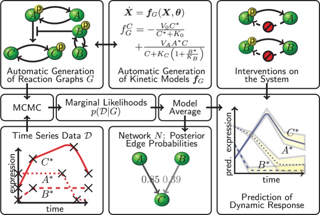
CheMA. Chemical reaction graphs G summarize interplay that is described quantitatively by kinetic equations ${\mathit{f}}_G$. Candidate graphs G are scored against observed time course data $\mathcal{D}$ in a Bayesian framework. A network N gives a coarse summary of the system; marginal posterior probabilities of edges in N quantify evidence in favor of causal relationships. The reaction graph G (and N) is treated as an unknown, latent object and the methodology allows Bayesian prediction of dynamics (including under intervention) in the unknown graph setting

2.1 Automatic generation of reaction graphs G

We construct reaction graphs for p proteins $\{X_1\dots X_p\}=\mathcal{V}$. Each X_i can be phosphorylated to $X_i^{*}$; the set of phosphorylated proteins is ${\mathcal{V}}^{*}$. Phosphorylation reactions $X_i\to X_i^{*}$ are catalyzed by enzymes $E\in {\mathcal{E}}_i$; the subscript indicates that each protein may have a specific set of enzymes (kinases). We consider the case in which the kinases themselves are phosphorylated proteins, i.e. ${\mathcal{E}}_i\subseteq {\mathcal{V}}^{*}$ (if phosphorylation of X_i is not driven by an enzyme in ${\mathcal{V}}^{*}$, we set ${\mathcal{E}}_i=\varnothing$). For simplicity, we do not consider multiple phosphorylation sites, other post-translational modifications (e.g. ubiquitinylation), protein degradation or spatial effects. The ability of enzyme $E\in {\mathcal{E}}_i$ to catalyze phosphorylation of X_i may be inhibited by proteins $I\in {\mathcal{I}}_{i,E}\subseteq {\mathcal{V}}^{*}$; the double subscript indicates that inhibition is specific to both target X_i and enzyme E (see below).

The reaction graph G provides a visual representation of the sets ${\mathcal{E}}_i$ and ${\mathcal{I}}_{i,E}$; Figure 1 shows an illustrative example on three proteins A, B and C. A causal biological network N(G) is formed by drawing exactly p vertices and edges (i, j) indicating that $X_i^{*}$ is either an enzyme catalyzing phosphorylation of X_j, or an inhibitor of such an enzyme. That is, $(i,j)\in N\iff i\in {\mathcal{E}}_j\vee \exists E·i\in {\mathcal{I}}_{j,E}$. For the example shown in Figure 1, the corresponding network N is the directed graph $A\to C\leftarrow B$.

2.2 Automatic generation of kinetic models ${\mathit{f}}_G$

The reaction graph G can be decomposed into local graphs G_i describing enzymes (and their inhibitors) for phosphorylation of protein X_i. For simplicity of exposition, we consider inference concerning G_i. Thus, X_i plays the role of the substrate; following conventional notation in enzyme kinetics, we refer to X_i using the symbol S and use [·] to denote concentration of the chemical species indicated by the argument.

We use kinetic models ${\mathit{f}}_G$ based on Michaelis–Menten functionals (Leskovac, 2003). Here we restrict attention to a relatively simple model class, but more complex dynamics could be incorporated. The rate of phosphorylation due to kinase E is given by $V_E[E]{[S]}^h/({[S]}^h+K_E^h)$, which acknowledges variation of kinase concentration [E] and permits kinase-specific response profiles, parameterized by K_E and h, with rate constant V_E. Below, the Hill coefficient h is taken equal to 1 (non-cooperative binding). We consider competitive inhibition, where substrate and inhibitor I compete for the same binding site on the enzyme ($EI\rightleftharpoons E\rightleftharpoons ES\to E+S^{*}$). When multiple inhibitors are present, they are assumed to act exclusively, competing for the same binding site on the enzyme ($EI\rightleftharpoons E\rightleftharpoons EI\prime$), corresponding mathematically to a rescaling of the Michaelis–Menten parameter $K_E\mapsto K_E(1+\sum _{I\in {\mathcal{I}}_{S,E}}[I]/K_I)$. We do not model phosphatase specificity; in particular, dephosphorylation is assumed to occur at a rate $V_0[S^{*}]/([S^{*}]+K_0)$, depending on a Michaelis–Menten parameter K₀ and taking a maximal value V₀.

Combining these assumptions produces a kinetic model for phosphorylation of substrate S, given by $f_{G,S}(\mathit{X},{\mathit{\theta }}_S)=$

$$-\frac{V_0[S^{*}]}{[S^{*}]+K_0}+{\displaystyle \sum _{E\in {\mathcal{E}}_S}\frac{V_E[E][S]}{[S]+K_E\left(1+{\displaystyle \sum _{I\in {\mathcal{I}}_{S,E}}\frac{[I]}{K_I}}\right)}}$$ (2)

where the parameter vector ${\mathit{\theta }}_S$ contains the maximum rates V and Michaelis–Menten constants K, and the (local) graph G_S specifies the sets ${\mathcal{E}}_S$ and ${\mathcal{I}}_{S,E}$. The complete dynamical system ${\mathit{f}}_G$ is given by taking, for each species $S\in \mathcal{V}$, a model akin to Equation (2). In this way, we are able to automate the generation of candidate parametric ODE models.

2.3 Model averaging and the network N

Evidence for a causal influence of protein i on protein j is summarized by the marginal posterior probability of a directed edge (i, j) in the network N. This is obtained by averaging over all possible reaction graphs G, as

$$p((i,j)\in N|\mathcal{D})=\frac{{\displaystyle \sum _{G:i\in G_j}p}(\mathcal{D}|G)p(G)}{{\displaystyle \sum _{G}p}(\mathcal{D}|G)p(G)}.$$ (3)

We note that while the marginal posterior in Equation (3) is an intuitive summary, the full posterior over reaction graphs G is also available for more detailed exploration. In the same vein, model averaging is used to compute posterior predictive distributions (see Supplementary Material).

Following work in structural inference for graphical models (Ellis and Wong, 2008), we bound graph in-degree; in particular, we consider only those sets of kinases ${\mathcal{E}}_S\subseteq {\mathcal{V}}^{*}$ that satisfy $|{\mathcal{E}}_S|\le c_1$, and similarly, we bound the number of inhibitors $|{\mathcal{I}}_{S,E}|\le c_2$ (see Section 3.1 below).

Bayesian variable selection requires multiplicity correction to control the false discovery rate and avoid degeneracy (Scott and Berger, 2010). For phosphorylation networks, we achieve multiplicity correction using a prior p(G) uniform over the number of kinases, and for a given kinase, uniform over the number of kinase inhibitors:

$$p(G)={\displaystyle \prod _{i=1}^p{\left(\begin{array}{c}p\\ |{\mathcal{E}}_i|\end{array}\right)}^{-1}}{\displaystyle \prod _{E\in {\mathcal{E}}_i}{\left(\begin{array}{c}p\\ |{\mathcal{I}}_{i,E}|\end{array}\right)}^{-1}}$$ (4)

We note that the above prior does not include biological knowledge concerning specific edges; informative structural priors are also available in the literature (Mukherjee and Speed, 2008).

2.4 Statistical formulation: CheMA 1.0

2.4.1 Time course data

Data $\mathcal{D}$ comprise measurements $y_i(t_j)$ and $y_i^{*}(t_j)$ proportional to the concentrations of unphosphorylated and phosphorylated forms, respectively, of protein i at discrete times t_j, $0\le j\le n$. Data are scale normalized to give unit mean for each protein ($\sum _j{y}_i(t_j)=\sum _j{y}_i^{*}(t_j)=n+1$). In CheMA 1.0, observables are related to dynamics via ‘gradient matching’. We follow Äijö and Lähdesmäki (2010); Bansal et al. (2006); Oates and Mukherjee (2012) and use a simple Euler scheme that approximates the gradient $d{X}_i/dt$ at time t_j by $z_i(t_j)=(y_i^{*}(t_j)-y_i^{*}(t_{j-1}))/(t_j-t_{j-1})$. We note that more accurate approximations could be used, at the cost of requiring more data points or additional modeling assumptions (see Section 4). The ODE model $f_{G,S}$ [Equation (2)] is formulated as a statistical model by constructing, conditional upon (unknown) Michaelis–Menten parameters K, a design matrix ${\mathit{D}}_{G,S}(\mathit{K})$ with rows

$$[-\frac{y_S^{*}}{y_S^{*}+K_0},\underset{E\in {\mathcal{E}}_S}{\underbrace{\dots ,\frac{y_E^{*}{y}_S}{y_S+K_E\left(1+\sum _{I\in {\mathcal{I}}_{S,E}}\frac{y_I^{*}}{K_I}\right)},\dots }}]$$ (5)

and then interpreting Equation (2) statistically as

$${\mathit{z}}_S={\mathit{D}}_{G,S}(\mathit{K})\mathit{V}+\mathbf{ϵ},\mathbf{ϵ}\sim \mathcal{N}(\mathit{0},{\sigma }^2\mathit{I})$$ (6)

where ${\mathit{z}}_S={[z_S(t_1),\dots ,z_S(t_n)]}^T,\mathcal{N}$ denotes a normal density, ${\sigma }^2$ the noise variance, I the identity matrix and, as above, V is the vector of maximum reaction rates. The appropriateness of normality, additivity and the uncorrelatedness of errors necessarily depends on the data generating and measurement processes, as well as the time intervals $t_j-t_{j-1}$ between consecutive observations, as discussed in Oates and Mukherjee (2012). This approximation has the crucial advantage of rendering the local reaction graphs G_S statistically orthogonal, such that each may be estimated independently (see Hill et al., 2012). Iterating over $S\in \mathcal{V}$ permits inference concerning the complete reaction graph G.

2.4.2 MCMC and marginal likelihoods

CheMA 1.0 uses truncated normal priors ${\mathcal{N}}_T(\mathit{\mu },\mathbf{\Sigma })$ with parameters $\mathit{\mu },\mathbf{\Sigma }$ inherited from the corresponding untruncated distribution. Truncation ensures non-negativity of parameters, while normality facilitates partial conjugacy (see below); additional information on truncated normals is provided in the Supplementary Material. To simplify notation, we consider a specific variable S and candidate model G_S and omit the subscript in what follows. To elicit hyperparameters $\mathit{\mu },\mathbf{\Sigma }$, we follow Xu et al. (2010) and assume all processes occur on observable time and concentration scales, that is ${\mathit{\mu }}_{\mathit{V}},{\mathit{\mu }}_{\mathit{K}}\sim \mathcal{O}(1)$, reflecting that the data are normalized a priori. For prior covariance of Michaelis–Menten parameters ${\mathbf{\Sigma }}_{\mathit{K}}$, we assume independence of the components K_i, so that $p(\mathit{K})={\mathcal{N}}_T(\mathit{K};{\mathit{\mu }}_{\mathit{K}},\nu \mathit{I})$, where ${\mathit{\mu }}_{\mathit{K}},\nu$ are hyperparameters. For the prior covariance ${\mathbf{\Sigma }}_{\mathit{V}}$ of maximum reaction rates, we take a unit information formulation of the truncated g-prior, so that $p(\mathit{V}|\mathit{K},\sigma )={\mathcal{N}}_T(\mathit{V};{\mathit{\mu }}_{\mathit{V}},n{\sigma }^2{(\mathit{D}\prime \mathit{D})}^{-1})$ where $\mathit{D}={\mathit{D}}_{G,S}(\mathit{K})$ is the design matrix defined above. This implies that the prior contributes (approximately) the same amount of information as one data point, as recommended by Kass and Wasserman (1995), and automatically selects the scale of the prior covariance (see Zellner, 1986). For the noise parameter, we use a Jeffreys prior $p(\sigma )\propto 1/\sigma$. These latter choices render the formulation partially conjugate, permitting an efficient Metropolis-within-Gibbs Markov chain Monte Carlo (MCMC) sampling scheme for the parameter posterior distribution, as described in detail in the Supplementary Material.

To estimate marginal likelihoods from sampler output, we exploit partial conjugacy and use the method of Chib and Jeliazkov (2001). As inference in CheMA 1.0 decomposes over proteins $X_i\in \mathcal{V}$, and for a given protein, over local models G_i, the computations were parallelized (full details and software provided as Supplementary Material). Alternatively, MCMC could be used over the discrete space of reaction graphs (Ellis and Wong, 2008) or the joint space of graphs and parameters (Oates et al., 2012).

2.4.3 Interventions on the system

In interventional experiments, data are obtained under treatments that externally influence network edges or nodes. Inhibitors of protein phosphorylation are now increasingly available; such inhibitors typically bind to the kinase domain of their target, preventing enzymatic activity. We consider such inhibitors in biological experiments below. Within CheMA 1.0, we model inhibition by setting to zero those terms in the design matrix ${\mathit{D}}_{G,S}$ corresponding to the inhibited enzyme E in the treated samples (‘perfect certain’ interventions in the terminology of Eaton and Murphy, 2007; Spencer et al., 2012). This removes the causal influence of E for the inhibited samples.

3 RESULTS

3.1 Hyperparameter specification and sensitivity

For CheMA 1.0, we set hyperparameters ${\mathit{\mu }}_{\mathit{V}}={\mathit{\mu }}_{\mathit{K}}=\mathit{1},\nu =1/2$ and the maximum in-degree constraint $c_1=2$; we investigated sensitivity by varying these parameters within (i) a toy model of signaling (Supplementary Fig. S3a–c) and (ii) in a subset of the simulations reported below (Supplementary Fig. S2). As the action of inhibition is second order in the Taylor expansion sense, inference for inhibitor variables ${\mathcal{I}}_{S,E}$ may be expected to require substantially more data, in line with the ‘weak identifiability’ of second-order terms reported in Calderhead and Girolami (2011). A preliminary investigation based on a toy model of signaling revealed that at typical sample sizes inference for inhibitor sets ${\mathcal{I}}_{S,E}$ was extremely challenging (Supplementary Fig. S3d). Combined with computational considerations, we decided to fix $c_2=0$ for subsequent experiments; that is, we did not include inhibitory regulation in the reaction graph. Further diagnostics, including MCMC convergence, are presented in the Supplementary Material.

3.2 In silico MAPK pathway

Data were generated from a mechanistic model of the MAPK signaling pathway described by Xu et al. (2010), specified by a system of 25 ODEs of Michaelis–Menten type whose reaction graph is shown in Figure 2a. This archetypal protein signaling system provides an ideal test bed, as the causal graph is known, and the model has been validated against experimentally obtained data (Xu et al., 2010). Following Oates and Mukherjee (2012), the Xu et al. model was transformed into a stochastic differential equation with intrinsic noise σ. Full details of the simulation setup appear in Supplementary Material.

Fig. 2.

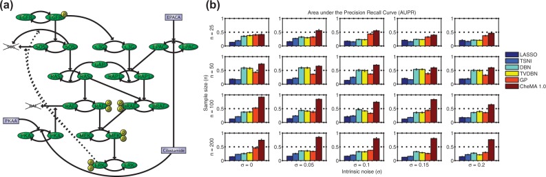
Network inference, simulation study. (a) Reaction graph G for the MAPK signaling pathway because of Xu et al. (2010). (The model, based on enzyme kinetics, uses Michaelis–Menten equations to capture a variety of post-translational modifications including phosphorylation.) (b) AUPR[with respect to the true causal network N(G)] for varying sample size n and noise level σ. [Network inference methods: (i) LASSO, ${\ell }_1$-penalized regression, (ii) TSNI, ${\ell }_2$-penalized regression, (iii) DBN, dynamic Bayesian networks, (iv) TVDBN, time-varying DBNs, (v) GP, non-parametric regression, (vi) CheMA 1.0, based on chemical kinetic models. Error bars display standard error computed over five independent datasets. (Full details provided in Supplementary Material.)

For inference of the network N(G), we compared our approach with existing network inference methods that are compatible with time course data: (i) ${\ell }_1$-penalized regression (‘LASSO’), (ii) time series network identification (‘TSNI’; Bansal et al. 2006; this is based on ${\ell }_2$-penalized regression), (iii) dynamic Bayesian networks (‘DBN’; Hill et al., 2012), (iv) time-varying DBNs (Dondelinger et al., 2012) and (v) Gaussian process regression with model averaging (‘GP’; Äijö and Lähdesmäki, 2010). Approaches (i–iii) are based on linear difference equations; (iv) relaxes the linear assumption in a piecewise fashion, whereas (v) is a semiparametric variable selection technique. We note that because TSNI cannot deal with multiple time courses, we adapted it for use in this setting. Implementation details for all methods may be found in the Supplementary Material.

To systematically assess estimation of network structure, we computed the average area under the precision-recall (AUPR) and area under the receiver-operating characteristic (AUROC) curves. Figure 2b shows mean AUPR for all approaches, for 20 regimes of sample size n and noise σ. CheMA 1.0 performs consistently well in all regimes, and outperforms (i–v) substantially at the larger sample sizes. It is interesting to note that the linear and piecewise linear DBNs (iii–iv) perform better at moderate sample sizes compared with higher sample sizes, possibly because of model misspecification. AUROC results (Supplementary Fig. S6) showed a broadly similar pattern, with CheMA 1.0 offering gains at larger sample sizes. For the kinetic parameters, however, we found that CheMA 1.0 struggled to precisely recover the true values $\mathit{\theta }=\{\mathit{V},\mathit{K}\}$, even when the reaction graph G was known (Fig. 3). The posterior distribution over rate constants V was much more informative than the posterior distribution over Michaelis–Menten parameters K, consistent with the ‘weak identifiability’ of kinase inhibitors that we found in Section 3.1.

Fig. 3.

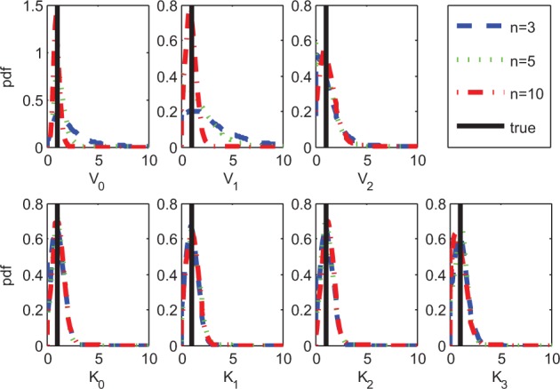
Posterior distributions over kinetic parameters when the graph G is known. As the number of samples n increases, the posterior mass concentrates on the true values much faster for the maximum reaction rates V (top row) than for the Michaelis–Menten parameters K (bottom row)

To investigate dynamical prediction in the setting where neither reaction graph nor parameters are known, we generated data from an unseen intervention and assessed ability to predict the resulting dynamics (details of the simulation are included in the Supplementary Material). To fix a length scale, both true and predicted trajectories were normalized by maximum protein expression in the test data. The quality of a predicted trajectory was then measured by the mean squared error (MSE) relative to the (held out) data points. The network inference approaches (i–v) above cannot be directly applied for prediction in this setting (although they could in principle be adapted to do so). Therefore, we compared CheMA 1.0 with the analogous linear formulation, that replaces Equation (2) by $f_{G,S}(\mathit{X},{\mathit{\theta }}_S)={\beta }_0+\sum _{E\in {\mathcal{E}}_S}{\beta }_E[X_E^{*}]$ (see Supplementary Material for details), along with a simple, baseline estimator (the ‘stationary benchmark’) that presumes protein concentrations do not change with time. Figure 4a displays predictions for the dynamics that result from EPAC inhibition. Here CheMA 1.0 provides qualitatively correct prediction, whereas the linear analogue rapidly diverges to infinity (due to poorly estimated eigenvalues). Therefore, we focused only on short-term prediction, specifically the first 25% of the time course, for which linear models may yet prove useful. Over all simulation regimes and experiments, including at small sample sizes, we found that our approach produced significantly lower MSE than both the linear and benchmark models (${\text{MSE}}_{\text{CheMA 1}.\text{0}}=0.061,{\text{MSE}}_{\text{Lin}.}=2.55,{\text{MSE}}_{\text{Bench}.}=0.199$). Furthermore, CheMA 1.0 consistently produced lowest MSE at all fixed values of n and σ (Supplementary Fig. S10; P < 0.001 binomial test).

Fig. 4.

Predicting dynamical response to a novel intervention: (a) predicting the effect of EPAC inhibition under the data generating model of Xu et al. (2010). [CheMA (solid) regions correspond to standard deviation of the posterior predictive distribution. Linear (dashed) replaces the non-linear chemical kinetic models with simple linear models. The stationary benchmark (dotted) simply uses the initial data point as an estimate for all later data points. The true test data are displayed as crosses. Here n = 100, $\sigma =0.1$.] (b) Assessing prediction over a panel of 15 breast cancer cell lines. (Training data were time series under treatment with a single inhibitor; test data represented a second held-out inhibitor. Normalized MSE was averaged over all protein species and all time points.)

3.3 In Vitro signaling

Next, we considered experimental data obtained using reverse-phase protein arrays (Hennessy et al., 2010) from 15 human breast cancer cell lines, of which 10 were of HER2+ subtype (Neve et al., 2006). These data comprised observations for key phosphoproteins AKT, EGFR, MEK, GSK3ab, S6, 4EBP1 and their unphosphoryated counterparts. Data were acquired under pretreatment with inhibitors Lapatinib (‘EGFRi’; an EGFR/HER2 inhibitor), GSK690693 (‘AKTi’; an AKT inhibitor) and without inhibition (DMSO) at 0.5, 1, 2, 4 and 8 h following serum stimulation, giving n = 15 observations of each species in each cell line (see Supplementary Material for full experimental protocol).

Assessment of inferred network topologies for the cell lines is challenging because the true cell line-specific networks are not known. Inferred topologies partially agree with known signaling (Supplementary Fig. S11), but the latter is based mainly on studies using wild-type cells and may not reflect networks in genetically perturbed cancer lines. Therefore, to assess performance, we also considered the problem of prediction of trajectories under an unseen intervention, where objective assessment is possible. We sought to compare performance of CheMA 1.0 against a literature-based ODE model (reaction graph G fixed according to literature and dynamics ${\mathit{f}}_G$ as described above) fitted to training data. No prior information concerning specific chemical reactions was provided to CheMA 1.0. This problem is highly non-trivial because of the small sample size, uneven sampling times and the complex observation process associated with proteomic assay data.

Training on DMSO and EGFRi (or AKTi) data, we assessed ability to predict the full dynamic response to AKT (or EGFR) inhibition. In this way, each held-out test set contained trajectories under a completely unseen intervention. By considering all 15 cell lines, giving 30 held-out datasets, we found that in 19 of 30 prediction problems CheMA 1.0 outperformed the literature predictor (Fig. 4b). As expected (and as in the case of the simulated data), the linear model was not well behaved for prediction (Supplementary Fig. S12) and is not shown. In the AKTi test, of the 10 HER2+ cell lines, 9 were better predicted by CheMA 1.0 compared with literature prediction (P = 0.01, binomial test; ${\text{MSE}}_{\text{CheMA 1}.\text{0}}=0.064$ versus ${\text{MSE}}_{\text{Lit}.}=0.274$). Conversely, four of five HER2− lines were better predicted by literature (${\text{MSE}}_{\text{Lit}.}=0.145$ versus ${\text{MSE}}_{\text{CheMA 1}.\text{0}}=0.240$), suggesting that signaling network topology in HER2+ lines may differ to the (wild type) literature topology, in line with the literature on the cell lines (Neve et al., 2006). This is encouraging from the perspective of CheMA, as a priori it is far from clear whether the training data, which involved only P = 6 species and n = 10 data points, contain sufficient information to predict the effect of an unseen intervention, even approximately. However, in two of the failure cases (HCC 1569, HCC 1954; EGFRi test) CheMA 1.0 produced extremely poor predictions (${\text{MSE}}_{\text{CheMA 1}.\text{0}}>1$), likely because of the small training sample size.

4 DISCUSSION

We proposed a general framework for using chemical kinetics in network inference and dynamical prediction. The use of chemical kinetics can be expected to contribute gains in causal inference because the underlying models are not structurally symmetric, allowing causal directionality to be established (Peters et al., 2011). In empirical results, we found that while CheMA 1.0 struggled to identify kinetic parameters from data, it was nevertheless able to identify the causal network; this discrepancy is explained by the fact that the latter is in a sense a projection of the former, and can be identifiable even when the full set of parameters are not.

An important challenge in systems biology is to predict the effect on signaling of a novel intervention, such as a drug treatment. At present, dynamical predictions in systems biology require a known chemical reaction graph, for instance, taken from the literature; a system of ODEs is usually specified based on such a graph and used for prediction. However, in many settings, the chemical reaction graph may differ depending on cell type or disease state and cannot be assumed known. In contrast, CheMA shows how prediction of dynamical behavior may be possible even when the reaction graph itself is unknown a priori. Unlike more convenient linear or discrete formulations, our use of chemical kinetic models provides interpretable predictions. For example, the dynamic behavior of phosphoprotein concentrations obtained under chemical kinetic rate laws is physically plausible (i.e. smooth, bounded and non-negative). Furthermore, by averaging predictions over reaction graphs, our approach should provide robustness in (typical) situations where it is unreasonable to expect to identify G precisely. Nevertheless, prediction of trajectories based on the protein data was challenging, likely because of noise and small sample sizes (Supplementary Fig. S13). We anticipate that continuing technical advances will move high-throughput proteomics closer to the favorable simulation regimes in Section 3.2 on which we found the richer non-linear models to be useful.

Several improvements can be made to the CheMA 1.0 implementation reported here, of which we highlight two: (i) gradient matching (rather than numerical solution of the automatically generated dynamical systems) can help to relieve the computational demands associated with exploration the large model spaces, but the Euler approximations we used for this purpose are crude. Improved gradient matching should be possible (at the expense of requiring more time points) via higher-order expansions, or (at the expense of additional modeling assumptions) kernel regression, the penalized likelihood approaches of González et al. (2013); Ramsay et al. (2007), or the Bayesian approach of Dondelinger et al. (2013). (ii) CheMA 1.0 does not explicitly distinguish between process noise and observation noise; an interesting direction for further research would be to incorporate an explicit observation model.

Two ongoing challenges in Bayesian computation relevant to CheMA include inference of model parameters and computation of marginal likelihoods for model selection. The second is an active area of research, with candidate approaches including variational approximations (Rue et al., 2009) and MCMC (Vyshemirsky and Girolami, 2008). In general, the computational burden of CheMA will be higher than many methods (see Supplementary Material). By way of illustration, Bayesian inference and prediction for a system of 27 protein species required over 12 h (serial) computational time. In contrast, linear or discrete models offer better scalability to high-dimensional settings. Thus, CheMA can complement existing methodologies but is not at present applicable to truly high-dimensional problems with hundreds or thousands of nodes.

Finally, we note the following caveats: (i) the automatic generation of kinetic equations limits the extent to which detailed knowledge about particular biochemical processes and dynamics may be incorporated. (ii) Our empirical results suggest that more complex interactions, including kinase inhibition, can be extremely difficult to identify in practice. (iii) The form of kinetics used here will likely be suboptimal when the assumptions of the Michaelis–Menten approximation are violated. (iv) Larger training and test datasets may be needed to allow truly effective trajectory prediction and comprehensive assessment of performance.

Funding: US Department of Energy (DE-AC02-05CH11231); US National Institute of Health, National Cancer Institute (U54 CA 112970, P50 CA 58207); UK Engineering and Physical Sciences Research Council (EP/E501311/1); and Netherlands Organisation for Scientific Research [Cancer Systems Biology Center].

Conflicts of interest: none declared.

REFERENCES

- Äijö T, Lähdesmäki H. Learning gene regulatory networks from gene expression measurements using non-parametric molecular kinetics. Bioinformatics. 2010;25:2937–2944. doi: 10.1093/bioinformatics/btp511. [DOI] [PubMed] [Google Scholar]
- Bansal M, et al. Inference of gene regulatory networks and compound mode of action from time course gene expression profiles. Bioinformatics. 2006;22:815–822. doi: 10.1093/bioinformatics/btl003. [DOI] [PubMed] [Google Scholar]
- Calderhead B, Girolami M. Statistical analysis of nonlinear dynamical systems using differential geometric sampling methods. J. R. Soc. Interface Focus. 2011;1:821–835. doi: 10.1098/rsfs.2011.0051. [DOI] [PMC free article] [PubMed] [Google Scholar]
- Chen WW, et al. Input-output behavior of ErbB signaling pathways as revealed by a mass action model trained against dynamic data. Mol. Syst. Biol. 2009;5:239. doi: 10.1038/msb.2008.74. [DOI] [PMC free article] [PubMed] [Google Scholar]
- Chib S, Jeliazkov I. Marginal likelihood from the metropolis-hastings output. J. Am. Stat. Assoc. 2001;96:270–281. [Google Scholar]
- Dondelinger F, et al. Non-homogeneous dynamic Bayesian networks with Bayesian regularization for inferring gene regulatory networks with gradually time-varying structure. Mach. Learn. 2012;90:191–230. [Google Scholar]
- Dondelinger F, et al. Sixteenth International Conference on Artificial Intelligence and Statistics, Scottsdale, AZ, USA. 2013. ODE parameter inference using adaptive gradient matching with Gaussian processes; pp. 216–228. [Google Scholar]
- Eaton D, Murphy K. Exact Bayesian structure learning from uncertain interventions. 11th International Conference on Artificial Intelligence and Statistics. 2007;Vol. 2:107–114. [Google Scholar]
- Ellis B, Wong W. Learning causal bayesian network structures from experimental data. J. Am. Stat. Assoc. 2008;103:778–789. [Google Scholar]
- Gardner T, et al. Inferring genetic networks and identifying compound mode of action via expression profiling. Science. 2003;301:102–105. doi: 10.1126/science.1081900. [DOI] [PubMed] [Google Scholar]
- González J, et al. Inferring latent gene regulatory network kinetics. Stat. Appl. Genet. Mol. 2013;12:109–127. doi: 10.1515/sagmb-2012-0006. [DOI] [PubMed] [Google Scholar]
- Hennessy BT, et al. A technical assessment of the utility of reverse phase protein arrays for the study of the functional proteome in nonmicrodissected human breast cancer. Clin. Proteomics. 2010;6:129–151. doi: 10.1007/s12014-010-9055-y. [DOI] [PMC free article] [PubMed] [Google Scholar]
- Hill SM, et al. Bayesian inference of signaling network topology in a cancer cell line. Bioinformatics. 2012;28:2804–2810. doi: 10.1093/bioinformatics/bts514. [DOI] [PMC free article] [PubMed] [Google Scholar]
- Honkela A, et al. Model-based method for transcription factor target identification with limited data. Proc. Natl Acad. Sci. USA. 2010;107:7793–7798. doi: 10.1073/pnas.0914285107. [DOI] [PMC free article] [PubMed] [Google Scholar]
- Kass RE, Wasserman L. A reference Bayesian test for nested hypotheses and its relationship to the Schwarz criterion. J. Am. Stat. Assoc. 1995;90:928–934. [Google Scholar]
- Kholodenko B. Cell-signalling dynamics in time and space. Nat. Rev. Mol. Cell Biol. 2006;7:165–176. doi: 10.1038/nrm1838. [DOI] [PMC free article] [PubMed] [Google Scholar]
- Leskovac V. Comprehensive Enzyme Kinetics. New York: Kluwer Academic/Plenum Publishers; 2003. [Google Scholar]
- Maathuis MH, et al. Estimating high-dimensional intervention effects from observational data. Ann. Stat. 2009;37:3133–3164. [Google Scholar]
- Mukherjee S, Speed T. Network inference using informative priors. Proc. Natl Acad. Sci. USA. 2008;105:14313–14318. doi: 10.1073/pnas.0802272105. [DOI] [PMC free article] [PubMed] [Google Scholar]
- Nachman I, et al. Inferring quantitative models of regulatory networks from expression data. Bioinformatics. 2004;20:i248–i256. doi: 10.1093/bioinformatics/bth941. [DOI] [PubMed] [Google Scholar]
- Nelander S, et al. Models from experiments: combinatorial drug perturbations of cancer cells. Mol. Syst. Biol. 2008;4:216. doi: 10.1038/msb.2008.53. [DOI] [PMC free article] [PubMed] [Google Scholar]
- Neve R, et al. A collection of breast cancer cell lines for the study of functionally distinct cancer subtypes. Cancer Cell. 2006;10:515–527. doi: 10.1016/j.ccr.2006.10.008. [DOI] [PMC free article] [PubMed] [Google Scholar]
- Oates CJ, Mukherjee S. Network inference and biological dynamics. Ann. Appl. Stat. 2012;6:1209–1235. doi: 10.1214/11-AOAS532. [DOI] [PMC free article] [PubMed] [Google Scholar]
- Oates CJ, et al. Network inference using steady state data and Goldbeter-Koshland kinetics. Bioinformatics. 2012;28:2342–2348. doi: 10.1093/bioinformatics/bts459. [DOI] [PMC free article] [PubMed] [Google Scholar]
- Pearl J. Causal inference in statistics: an overview. Stat. Surv. 2009;3:96–146. [Google Scholar]
- Peters J, et al. 27th Conference on Uncertainty in Artificial Intelligence, Barcelona, Spain. 2011. Identifiability of causal graphs using functional models; pp. 589–598. [Google Scholar]
- Ramsay JO. Parameter estimation for differential equations: a generalized smoothing approach. J. R. Stat. Soc. Series B Stat. Methodol. 2007;69:741–796. [Google Scholar]
- Rue H, et al. Approximate Bayesian inference for latent Gaussian models using integrated nested laplace approximations. J. R. Stat. Soc. Series B Stat. Methodol. 2009;71:319–392. [Google Scholar]
- Sachs K, et al. Causal Protein-signaling networks derived from multiparameter single-cell data. Science. 2005;308:523–529. doi: 10.1126/science.1105809. [DOI] [PubMed] [Google Scholar]
- Scott JG, Berger JO. Bayes and empirical-bayes multiplicity adjustment in the variable-selection problem. Ann. Stat. 2010;38:2587–2619. [Google Scholar]
- Spencer SEF, et al. CRiSM Working Paper. Coventry, UK: University of Warwick; 2012. Dynamic Bayesian networks for interventional data. [Google Scholar]
- Vyshemirsky V, Girolami M. Bayesian ranking of biochemical system models. Bioinformatics. 2008;24:833–839. doi: 10.1093/bioinformatics/btm607. [DOI] [PubMed] [Google Scholar]
- Werhli A, et al. Comparative evaluation of reverse engineering gene regulatory networks with relevance networks, graphical Gaussian models and Bayesian networks. Bioinformatics. 2006;22:2523–2531. doi: 10.1093/bioinformatics/btl391. [DOI] [PubMed] [Google Scholar]
- Xu T-R, et al. Inferring signaling pathway topologies from multiple perturbation measurements of specific biochemical species. Sci. Signal. 2010;3:ra20. [PubMed] [Google Scholar]
- Zellner A. On assessing prior distributions and Bayesian regression analysis with g-prior distributions. In: Goel PK, Zellner A, editors. Bayesian inference and decision techniques—Essays in honor of Bruno de Finetti, North-Holland, Amsterdam. 1986. pp. 233–243. [Google Scholar]
Associated Data
This section collects any data citations, data availability statements, or supplementary materials included in this article.