Empowering Imaging Biomarkers of Alzheimer’s Disease

Abstract

In a previous report, we proposed a method for combining multiple markers of atrophy caused by Alzheimer’s Disease (AD) into a single atrophy score that is more powerful than any one feature. We applied the method to expansion rates of the lateral ventricles, achieving the most powerful ventricular atrophy measure to date. Here, we expand our method’s application to Tensor Based Morphometry (TBM) measures. We also combine the volumetric TBM measures with previously computed ventricular surface measures into a combined atrophy score. We further show that our atrophy scores are longitudinally unbiased, with the intercept bias estimated at two orders of magnitude below the mean atrophy of control subjects at one year. Both approaches yield the most powerful biomarker of atrophy not only for ventricular measures, but for all published unbiased imaging measures to date. A two-year trial using our measures requires only 31 [22 43] AD subjects, or 56 [44 64] subjects with Mild Cognitive Impairment (MCI) to detect 25% slowing in atrophy with 80% power and 95% confidence.

1. Introduction

Imaging biomarkers of Alzheimer’s disease must offer sufficient power to detect brain atrophy in subjects scanned repeatedly over time (Cummings, 2010, Ross et al., 2012, Wyman et al., 2012). The expected cost of a drug trial may be prohibitively high, unless we can reasonably expect disease-slowing effects to be detected quickly enough and with reasonably few subjects. Imaging measures from standard structural MRI show considerable promise. Their use stems from the premise that longitudinal changes may be more precisely and reproducibly measured with MRI than comparable changes in clinical, CSF, or proteomic assessments; clearly, whether that is true depends on the measures used. The use of MRI in a drug trial has some caveats: most MR studies from published drug trials have detected no effect or even a small - and possibly irrelevant but significant - increase in atrophy in the treatment group. Brain measures that are helpful for diagnosis, such as PET scanning, may not be stable for large multi-center (N = several hundred) longitudinal trials that aim to slow disease progression. Other markers, such as CSF measures of amyloid and tau proteins to assess brain amyloid, may suffer the opposite problem of showing too little change during the clinical AD period. As a result, there is interest in testing the reproducibility of biomarkers, as well as methods to optimally combine them (Yuan et al., 2012).

Recent studies have tested the reproducibility and accuracy of a variety of MRI-derived measures of brain change. Several are highly correlated with clinical measures, and can predict future decline on their own, or in combination with other relevant measures. Although not the only important consideration, some analyses have assessed which MRI-based measures show greatest effect sizes for measuring brain change over time, while avoiding issues of bias and asymmetry that can complicate longitudinal image analysis (Fox et al., 2011, Holland et al., 2011, Hua et al., 2013), and while avoiding removing scans from the analysis that may lead to unfairly optimistic sample size estimates (Wyman et al., 2012, Hua et al., 2013). Promising MRI-based measures include the brain boundary shift integral (Schott et al., 2010, Leung et al., 2012), the ventricular boundary shift integral (Schott et al., 2010) and measures derived from anatomical segmentation software such as Quarc or FreeSurfer, some of which have been recently modified to handle longitudinal data more accurately (Fischl and Dale, 2000, Smith et al., 2002, Holland and Dale, 2011, Reuter et al., 2012).

Although several power estimates are possible, the analysis advocated by the ADNI Biostatistics Core (Beckett, 2000), is to estimate the minimal sample size required to detect, with 80% power, a 25% reduction in the mean annual change, using a two-sided test and standard significance level α = 0.05 for a hypothetical two-arm study (treatment versus placebo). The estimate for the minimum sample size is computed from the formula below. β̂ denotes the annual change (average across the group) and σ̂²_D refers to the variance of the annual rate of change.

$$n=\frac{2{{\widehat{\sigma }}^2}_D{\left(z_{1-\alpha /2}+z_{\mathit{power}}\right)}^2}{{\left(0.25\widehat{\beta }\right)}^2}$$ (1)

Here z_α is the value of the standard normal distribution for which P[Z < z_α] = α. The sample size required to achieve 80% power is commonly denoted by n80. Typical n80s for competitive methods are under 150 AD subjects and under 300 MCI subjects; the larger numbers for MCI reflect the fact that brain changes tend to be slower in MCI than AD and MCI is an etiologically more heterogeneous clinical category. For this reason, it is harder to detect a modification of changes that are inherently smaller, so greater sample sizes are needed to guarantee sufficient power to detect the slowing of disease.

Many algorithms can detect localized or diffuse changes in the brain, creating detailed 3D maps of changes (Leow et al., 2007, Avants et al., 2008, Shi et al., 2009), but the detail in the maps they produce is often disregarded when making sample size estimates according to (1), as the formula expects a single, univariate measure of change. In other words, it requires a single number, or ‘numeric summary’ to represent all the relevant changes occurring within the brain. To mitigate this problem, Hua et al. (Hua et al., 2009) defined a “statistical ROI” based on a small sample of AD subjects by thresholding the t-statistic of each feature (voxel) and summing the relevant features over the ROI; this approach was initially advocated in the FDG-PET literature to home in on regions that show greatest effects (Chen et al., 2010). In spirit, the statistical ROI is a rudimentary supervised learning approach, as it finds regions that show detectable effects in a training sample, and uses them to empower the analysis of future samples; the samples used are non-overlapping and independent, to avoid circularity. However, a simple threshold-based masking is known to potentially eliminate useful features, as binarisation loses a lot of the information present in continuous weights (Duda et al., 2001). While many studies have used machine learning to predict the progression of neurodegenerative diseases and differentiate diagnostic groups such as AD, MCI, and controls (Vemuri et al., 2008, Kohannim et al., 2010, Kloppel et al., 2012), we found no attempts in the literature that used learning to directly optimize power to detect brain change.

To address this issue, we observed that minimizing (1) is exactly analogous to one-class Linear Discriminant Analysis. We applied the method to surface-based longitudinal expansion rates of the ventricular boundary (Gutman et al., 2013), achieving the lowest sample size estimates of any ventricle-based measure of AD to date, both in terms of absolute and control-adjusted atrophy. Here, we apply the LDA-based weighting to recently reported maps of whole brain volume change based on Tensor Based Morphometry (Hua et al., 2013). Further, we combine ventricular surface and TBM volume measures into one combined atrophy score. Our results show a marked improvement over the stat-ROI approach, achieving substantively lower sample size estimates than any ADNI-based report to date.

2. Materials and Methods

2.1. Alzheimer’s Disease Neuroimaging Initiative

Data used in the preparation of this article were obtained from the Alzheimer’s Disease Neuroimaging Initiative (ADNI) database (adni.loni.ucla.edu). The ADNI was launched in 2003 by the National Institute on Aging (NIA), the National Institute of Biomedical Imaging and Bioengineering (NIBIB), the Food and Drug Administration (FDA), private pharmaceutical companies and non-profit organizations, as a $60 million, 5-year public-private partnership. The primary goal of ADNI has been to test whether serial magnetic resonance imaging (MRI), positron emission tomography (PET), other biological markers, and clinical and neuropsychological assessment can be combined to measure the progression of mild cognitive impairment (MCI) and early Alzheimer’s disease (AD). Determination of sensitive and specific markers of very early AD progression is intended to aid researchers and clinicians to develop new treatments and monitor their effectiveness, as well as lessen the time and cost of clinical trials.

The Principal Investigator of this initiative is Michael W. Weiner, MD, VA Medical Center and University of California – San Francisco. ADNI is the result of efforts of many co-investigators from a broad range of academic institutions and private corporations, and subjects have been recruited from over 50 sites across the U.S. and Canada. The initial goal of ADNI was to recruit 800 adults, ages 55 to 90, to participate in the research, approximately 200 cognitively normal older individuals to be followed for 3 years, 400 people with MCI to be followed for 3 years and 200 people with early AD to be followed for 2 years. For up-to-date information, see www.adni-info.org.

Longitudinal brain MRI scans (1.5 Tesla) and associated study data (age, sex, diagnosis, genotype, and family history of Alzheimer’s disease) were downloaded from the ADNI public database (http://www.loni.ucla.edu/ADNI/Data/) on July 1^st 2012. The first phase of ADNI, i.e., ADNI-1, was a five-year study launched in 2004 to develop longitudinal outcome measures of Alzheimer’s progression using serial MRI, PET, biochemical changes in CSF, blood and urine, and cognitive and neuropsychological assessments acquired at multiple sites similar to typical clinical trials.

All subjects underwent thorough clinical and cognitive assessment at the time of scan acquisition. All AD patients met NINCDS/ADRDA criteria for probable AD (McKhann et al., 1984). The ADNI protocol lists more detailed inclusion and exclusion criteria (Mueller et al., 2005a, Mueller et al., 2005b), available online http://www.alzheimers.org/clinicaltrials/fullrec.asp?PrimaryKey=208). The study was conducted according to the Good Clinical Practice guidelines, the Declaration of Helsinki and U.S. 21 CFR Part 50-Protection of Human Subjects, and Part 56-Institutional Review Boards. Written informed consent was obtained from all participants before performing experimental procedures, including cognitive testing.

2.2. MRI acquisition and image correction

All subjects were scanned with a standardized MRI protocol developed for ADNI (Jack et al., 2008). Briefly, high-resolution structural brain MRI scans were acquired at 59 ADNI sites using 1.5 Tesla MRI scanners (GE Healthcare, Philips Medical Systems, or Siemens). Additional data was collected at 3-T, but is not used here as it was only collected on a subsample that is too small for making comparative assessments of power. Using a sagittal 3D MP-RAGE scanning protocol, the typical acquisition parameters were repetition time (TR) of 2400 ms, minimum full echo time (TE), inversion time (TI) of 1000 ms, flip angle of 8°, 24 cm field of view, 192×192×166 acquisition matrix in the x-, y-, and z-dimensions, yielding a voxel size of 1.25×1.25×1.2 mm³, later reconstructed to 1 mm isotropic voxels. For every ADNI exam, the sagittal MP-RAGE sequence was acquired a second time, immediately after the first using an identical protocol. The MP-RAGE was run twice to improve the chance that at least one scan would be usable for analysis and for signal averaging if desired.

The scan quality was evaluated by the ADNI MRI quality control (QC) center at the Mayo Clinic to exclude failed scans due to motion, technical problems, significant clinical abnormalities (e.g., hemispheric infarction), or changes in scanner vendor during the time-series (e.g., from GE to Philips). Image corrections were applied using a standard processing pipeline consisting of four steps: (1) correction of geometric distortion due to gradient non-linearity (Jovicich et al., 2006), i.e. “gradwarp” (2) “B1-correction” for adjustment of image intensity inhomogeneity due to B1 non-uniformity (Jack et al., 2008), (3) “N3” bias field correction for reducing residual intensity inhomogeneity (Sled et al., 1998), and (4) phantom-based geometrical scaling to remove scanner and session specific calibration errors (Gunter et al., 2006).

2.3. The ADNI-1 dataset

For our experiments, we analyzed data from 683 ADNI subjects with baseline and 1 year scans, and 542 subjects with baseline, 1 year and 2 year scans. The former group consisted of 144 AD subjects (age at screening: 75.5 +/− 7.4, 67 female (F)/77 male (M)), 337 subjects with Mild Cognitive Impairment (MCI) (74.9 +/− 7.2, 122 F/215 M), and 202 age-matched healthy controls (NC) (76.0 +/− 5.1, 95 F/107 M). The 2-year group (i.e., people with scans at baseline, and after a 1-year and 2-year interval) had 111 AD (75.7 +/− 7.3, 52 F/59 M), 253 MCI (74.9 +/− 7.1, 87 F/166 M), and 178 NC (76.2 +/− 5.2, 85 F/93 M) subjects. All raw scans, images with different steps of corrections, and the standard ADNI-1 collections are available to the general scientific community at http://www.loni.ucla.edu/ADNI/Data/. We used exactly all ADNI subjects available to us (on Feb. 1, 2012) who had both baseline and 12 month scans, and all subjects with 24 month scans (available July 1, 2012). The use of all subjects without data exclusion has been advocated by (Wyman et al., 2012) and (Hua et al., 2013), because any scan exclusion can lead to power estimates that are unfairly optimistic, and many drug trials prohibit the exclusion of any scans at all.

2.4 Surface Extraction and Analysis

Our surfaces were extracted from 9-parameter affine-registered, fully processed T1-weighted anatomical scans. We used a modified version of Chou’s registration-based segmentation (Chou et al., 2008), using inverse-consistent fluid registration with a mutual information fidelity term (Leow et al., 2007). To avoid issues of bias and non-transitivity, we segmented each of our subjects’ two or three scans separately. In this approach, a set of hand-labeled “templates” are aligned to each scan, with multiple atlases being used to greatly reduce error. There were two templates from each of the three diagnostic groups, with one male and one female subject in each. Ventricular surfaces were extracted using an inverse-consistent fluid registration with a mutual information fidelity term to align a set of hand-labeled ventricular templates to each scan. The template surfaces were registered as a group following a medial-spherical registration method (Gutman et al., 2012). To improve upon the standard multi-atlas segmentation, which generally involves a direct, or a weighted average of the warped binary masks, we select an individual template that best fits the new boundary at each boundary point. A naïve formulation of this synthesis can be written as below:

$$\mathit{S}(\mathit{p})={\sum }_{\mathit{i}}{\mathit{W}}^{\mathit{i}}(\mathit{p}){\mathit{T}}_{\mathit{i}}(\mathit{p}),{\mathit{W}}^{\mathit{i}}(\mathit{p})=\{\begin{array}{ll}\mathbf{1}\hfill & \hfill \mathit{if}\mathit{s}(\mathit{I},{\mathit{I}}_{\mathit{i}})[\mathit{p}]>\mathit{s}(\mathit{I},{\mathit{I}}_{\mathit{j}})[\mathit{p}]\forall \mathit{j}\ne \mathit{i}\\ \mathbf{0}\hfill & \hfill \mathit{otherwise}\end{array}.$$ (2)

Here, I, S are the new image and boundary surface, {I_i, T_i}_i are template surfaces and images warped to the new image, and s(I, I_i)[p] is some local normalized similarity measure at point p. Normalized mutual information around a neighborhood of each point was used to measure similarity. This approach allows for more flexible segmentation, in particular for outlier cases. Even a weighted average, with a single weight applied to each individual template, often distorts geometric aspects of the boundary that are captured in only a few templates, perhaps only in one. However, to enforce smoothness of the resulting surface, care must be taken around the boundaries of the surface masks Wⁱ. An effective approach is to smooth the masks with a spherical heat kernel, so that our final weights are ${\mathit{W}}_{\mathit{\sigma }}^{\mathit{i}}(\mathit{q})={\int }_{{\mathbb{S}}^2}{\mathit{K}}_{\mathit{\sigma }}(\mathit{p},\mathit{q}){\mathit{W}}^{\mathit{i}}(\mathit{p})\mathit{dp}$. This approach is similar to (Yushkevich et al., 2010b), differing mainly in the fact that it is a surface-based rather than a voxel-based approach.

Local surface-based maps of atrophy were then generated using the algorithm described in (Gutman et al., 2012, Gutman et al., 2013). Briefly, the algorithm deforms a curve to minimize the medial energy associated with the shape, which may be written as:

$$R(\mathit{c},{\mathit{c}}^{\prime },\mathcal{M})={\int }_0^1\underset{\mathit{p}\in \mathcal{M}}{\int }w(\mathit{c}(t),{\mathit{c}}^{\prime }(t),\mathit{p},\mathcal{M}){\mid \mathit{c}(t)-\mathit{p}\mid }^{2}d\mathcal{M}\mathit{dt},$$ (3)

The term w(c(t), c′(t), p, ) represents the medial weight for each pair of curve and surface points, which is described in detail in (Gutman et al., 2012). Two surface-based feature functions are generated based on the curve representing shape geometry: thickness and the global orientation function (GOF) (Gutman et al., 2012). We non-linearly register shapes first longitudinally and then to a mean template by parametrically minimizing sum of square differences (SSD) between corresponding feature functions. Our mean template is generated by averaging the hand-traced templates in a group-wise fashion as described in (Gutman et al., 2012). The thickness change maps represent change in the distance to the medial axis from any given point on the ventricular boundary, or intuitively, change in thickness of the shape.

2.5 Tensor-Based Morphometry

TBM is an image analysis technique that measures brain structural differences from the gradients of deformation fields that align one image to another (Freeborough and Fox, 1998, Ashburner and Friston, 2003, Leow et al., 2007). Individual Jacobian maps were created to estimate 3D patterns of structural brain change over time by warping the 9P-registered and ‘skull-stripped’ follow-up scan to match the corresponding screening scan. We used a non-linear inverse consistent elastic intensity-based registration algorithm (Leow et al., 2007), which optimizes a joint cost function based on mutual information (MI) and the elastic energy of the deformation. The deformation field was computed using a spectral method to implement the Cauchy–Navier elasticity operator (Marsden and Hughes, 1983, Thompson et al., 2000) using a Fast Fourier Transform (FFT) resolution of 64 × 64 × 64. This corresponds to an effective voxel size of 3.4 mm in the x, y, and z dimensions (220 mm/64 = 3.4 mm). Color-coded maps of the Jacobian determinants were created to illustrate regions of ventricular/CSF expansion (i.e., with det J(r) > 1), or brain tissue loss (i.e., with det J(r) < 1) over time. These longitudinal maps of tissue change were also spatially normalized across subjects by nonlinearly aligning all individual Jacobian maps to a Minimal Deformation Template (MDT), for regional comparisons and group statistical analyses. See (Hua et al., 2013) for more details.

2.6 LDA for Empowering Biomarkers

In designing an imaging biomarker, one generally seeks to balance the intuitiveness of the measure and its power to track disease progression. In this study, we choose to use, alternatively, radial expansion of the lateral ventricles, local tissue loss as measured by Jacobian determinants of non-linear longitudinal warps, or the combination of the two. Having made this choice, we would now like to find an optimal linear weighting for each surface vertex and image voxel to maximize the effect size of our combined global measure of change. A linear model may not have the intuitive clarity of a binary weighting (i.e., specifying or masking a restricted region to measure), but its meaning is still sufficiently clear and can be easily visualized. Thus we would like to minimize our sample size estimate (1) as a function of the weights, w:

$$n(\mathbf{w})=C\frac{\frac{1}{N-1}\mathrm{\sum }{({\mathbf{x}}_i^{\mathrm{T}}\mathbf{w}-{\mathbf{m}}^{\mathrm{T}}\mathbf{w})}^2}{{({\mathbf{m}}^{\mathrm{T}}\mathbf{w})}^2}=\frac{1}{N-1}C\frac{{\mathbf{w}}^{\mathrm{T}}{\mathbf{S}}_W\mathbf{w}}{{\mathbf{w}}^{\mathrm{T}}{\mathbf{S}}_B\mathbf{w}}.$$ (4)

Here C = 32(z_1−α/2 + z_power)², x_i is the thickness change for the i^th subject, m is the mean vector, the covariance matrix ${\mathbf{S}}_W={\sum }_{i=1}^N({\mathbf{x}}_i-\mathbf{m}){({\mathbf{x}}_i-\mathbf{m})}^T$, and S_B = mm^T. Minimizing (4) is equivalent to maximizing

$$J(\mathbf{w})=\frac{{\mathbf{w}}^{\mathrm{T}}{\mathbf{S}}_B\mathbf{w}}{{\mathbf{w}}^{\mathrm{T}}{\mathbf{S}}_W\mathbf{w}},$$ (5)

which is a special case of the LDA cost function, with a maximum given by

$$\mathbf{w}={\mathbf{S}}_W^{-1}\mathbf{m}.$$ (6)

For our purposes, m represents the mean of the diseased group. We denote this by m = m_AD,MCI, where m_AD,MCI stands for the mean expansion vector in the combined MCI and AD group. We make no distinction between these two groups during LDA training. Maximizing (5) directly is generally not stable when S_W has a high condition number. Further, when the feature space is large enough, as in the case of Jacobian fields with roughly 2 million features, storing the dense 2Mx2M covariance matrix directly simply becomes impossible. We resolve this issue by applying Principal Components Analysis (PCA) to our training sample, storing the first k principal components (PCs) in the rows of a matrix, P, and computing the corresponding k eigenvalues λ_j. This is a standard approach when applying LDA to actual two-class problems, as it makes the mixed covariance matrix nearly diagonal. In our case, the covariance in PCA space is exactly diagonal, which reduces (6) to a direct computation:

$$\mathbf{w}={\mathbf{P}}^{\mathrm{T}}\mathbf{\omega },\text{where}{\omega }_j={[\mathbf{Pm}]}_j/{\lambda }_j.$$ (7)

This approach is very fast: one can compute the first k eigenvectors and eigenvalues of S_W without explicitly computing S_W itself. While alternative, possibly more flexible basis function sets are possible, we choose PCA for its simplicity.

The order of subjects in each diagnostic group is randomly changed to eliminate the confound due to different scanning protocols at different ADNI acquisition sites.. This step is needed mainly to ensure a roughly equal distribution of sites in each fold, as ADNI subjects are ordered by site by default. Where the subjects are scanned is known to correlate with reliability in many morphometric measures, and we have found that our LDA measures are affected by the site distribution as well. This is only done once before LDA training, with the same order and same subdivision of diagnostic groups used for each method.

To validate our data-driven weighting approaches, we create two groups of equal size, with an equal number of MCI and AD subjects in each. Each of these folds is then used to optimize the number of principal components k. This is done by subdividing the training fold further into 2 sub-folds of equal size, computing principal components separately on each sub-fold, and training a different LDA model using all PC’s up to k, with k varying from 1 to the total number of subjects in the sub-fold. A sample size for each sub-fold’s model is computed by applying the linear weights to the other sub-fold. The optimal k is chosen so that the mean of the two sub-folds’ sample size estimates is minimized. Further, to avoid circularity, we do not use the six hand-traced subjects used in generating the ventricular surface template for model training or testing. For TBM, such circularity is avoided entirely, as the Minimum Distance Template (MDT) (Hua et al., 2008) is based on 40 control subjects, which are not used during the training or testing stages. This approach is an adaptation of the standard nested cross-validation technique in machine learning.

Because Jacobian determinants have a skewed distribution due to the nature of the measurement, we perform LDA training on the logarithm of the Jacobian maps, which in the first approximation is equivalent to actual atrophy rates over a given time interval. This step ensures that the Gaussian assumption in LDA is more closely satisfied.

3. Results

Below we compare the performance of our LDA-based vertex weighting of ventricular expansion (Medial Vent LDA), the LDA-based voxel weighting of TBM maps (TBM-LDA), the combination of the two LDA measures into one score, and the LDA Stat-ROI method previously reported on in (Hua et al., 2013). Though in general, absolute ventricular expansion may not be specific to AD pathology, its finely resolved surface-based signature is used here as a surrogate measure of AD-related atrophy in addition to what can be learned from TBM. In testing each of these weighting methods, we used nested 2-fold cross-validation. Only AD and MCI subjects were used in the training stage. Further, we restricted our training sample to include only 1-year changes. Twenty-four month data was only used for testing, applying 1-year models to the non-overlapping subgroups of the 24-month data. Tables 2a and 2b summarize sample size estimates for 1-year and 2-year clinical trials for each of the four biomarkers. The linear weight maps are visualized in Figures 1 and 2. To visualize the difference between a multivariate approach and a mass-univariate type of weighting as done in the stat-ROI approach, we also display maps of t-statistics in Figures 3 and 4. The t-maps were computed to test the null hypothesis that no change takes place among the AD and MCI subjects at each spatial location over one year. In another test, we restricted the PCA feature space to the gray matter voxels, segmented by BrainSuite (Shattuck et al., 2001), and computed the resulting power estimates. The weight maps are visualized in Figure 5. To assess the reproducibility of our sample sizes, we also computed bootstrapped 95% confidence intervals for our sample size estimates (DiCicio and Efron, 1996).

Table 2a. Sample size estimates for clinical trials, using anatomical biomarkers of change over 12 months as an outcome measure.

Depending on how we weight the features on the ventricular surfaces, the sample size estimates can be reduced, and the power of the study increased. “Whole” stands for whole-brain TBM of Figure 1, and “GM” means the TBM model restricted to gray matter, from Figure 5. Mean sample size estimates are computed as the average of the two folds’ estimates. 95% confidence intervals are presented in parentheses.

	MCI	AD	Mean MCI	Mean AD
Vent-LDA	111/96 (85,150)/(75,127)	65/86 (46,92)/(64,128)	104 (94,139)	75 (64,102)
TBM-LDA Whole	85/99 (67,110)/(77,131)	48/50 (34,70)/(35,85)	92 (77,111)	49 (38,66)
TBM-LDA GM	110/93 (85,145)/(73,122)	48/49 (33,74)/(35,76)	101 (84,122)	49 (37,64)
Vent + TBM	83/72 (66,112)/(56,92)	41/46 (28,65)/(32,68)	78 (63,90)	43 (33,58)
TBM stat-ROI	--	--	135 (114,167)	64 (51,86)

Table 2b. Sample size estimates for clinical trials, using anatomical biomarkers of change over 24 months as an outcome measure.

95% confidence intervals are presented in parentheses.

	MCI	AD	Mean MCI	Mean AD
Vent-LDA	80/62 (65,108)/(44,86)	67/47 (47,122)/(31,67)	71 (65,98)	57 (45,89)
TBM-LDA Whole	61/64 (47,81)/(50,81)	28/33 (19,44)/(21,56)	63 (52,75)	31 (22,43)
TBM-LDA GM	73/66 (58,92)/(51,88)	38/31 (25,60)/(19,51)	69 (57,81)	34 (25,47)
Vent + TBM	53/58 (40,72)/(46,73)	28/34 (19,43)/(22,62)	56 (44,64)	32 (22,44)
TBM stat-ROI	--	--	109 (92,131)	41 (33,55)

Figure 1.

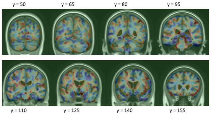
Log-Jacobian (TBM) LDA weighting, scaled by standard deviation of the weights. Red regions expect expansion, and blue – atrophy.

Figure 2.

Ventricular LDA weighting, scaled by standard deviation of the weights.

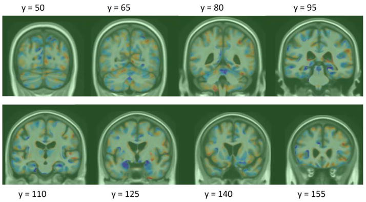
Figure 3.

Log-Jacobian (TBM) t-maps, based on the null hypothesis that there is no change over 1 year in AD and MCI subjects in each voxel. The difference between these maps and Figure 1 shows the difference between a multivariate and a mass-univariate approach in weighting Jacobian maps.

Figure 4.

Ventricular thickness t-maps, based on the null hypothesis that there is no change over 1 year in AD and MCI subjects at each mesh vertex. The difference between these maps and Figure 2 shows the difference between a multivariate and a mass-univariate approach in weighting Jacobian maps.

Figure 5.

Log-Jacobian (TBM) LDA weighting restricted to gray matter regions, scaled by standard deviation of the weights. Red regions expect expansion, and blue – atrophy.

For ventricular surface measures, the optimal number of principal components was found to be 28 and 47, for folds 1 and 2, respectively. For Jacobian maps, the smallest sample size was achieved at k = 115 and 103 for whole-brain LDA, and at k = 98 and 95 for LDA restricted to gray matter.

We compared the sample size estimates of the stat-ROI approach to TBM-LDA in table 4. The LDA measures significantly outperformed the stat-ROI measure for MCI subjects, and trended better for AD subjects.

Table 4. Bootstrapped p-values, stat-ROI vs. TBM-LDA measures.

Non-parametric test assessing the probability that the stat-ROI measure leads to lower or equal required sample size compared to the given LDA measure.

	12 months		24 months
	GM-LDA vs. stat-ROI	Whole LDA vs. stat-ROI	GM-LDA vs. stat-ROI	Whole LDA vs. stat-ROI
AD	0.0683	0.0795	0.162	0.0631
MCI	0.014	0.0019	0.0001	<0.0001

To assess whether there is any evidence of longitudinal bias of our weighted measures, we applied our 1 year models to healthy controls at 12 and 24 months. Using a method similar to (Hua et al., 2011), we used the y-intercept of the linear regression as a measure of bias (bearing in mind the caveats noted that there may be some biological acceleration or deceleration that could appear to be a bias). We again used bootstrapping to estimate the intercept and linear fit confidence intervals (DiCicio and Efron, 1996), with the exception of TBM stat-ROI, which we reprint from (Hua et al., 2013). We note that using standardized linear fit model CI’s leads to intervals that are more than twice as wide for the LDA models, implying that our CI’s are quite conservative. Figure 6 shows the regression plots for all LDA models over the two follow-up time points. Confidence intervals for the linear fits are shown in dotted green lines. The bias test results are summarized in Table 3. We note that the intercept shows virtually zero bias for all the LDA models, as it is two orders of magnitude lower than change in controls at 1 year.

Figure 6. Regression plots for LDA-based atrophy measures in controls.

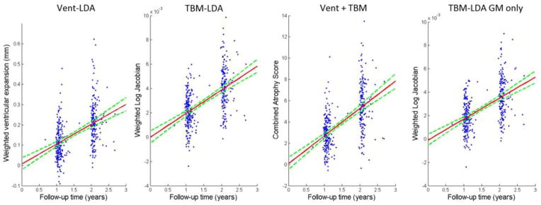
95% confidence belts for the regression models are shown with dotted green lines. All LDA models are longitudinally unbiased, since the zero intercept is contained in the 95% confidence interval on the intercept, for each of the methods.

Table 3. Longitudinal bias analysis of AD imaging biomarkers.

Change in healthy controls is linearly regressed over two time points. The intercept is very close to zero, with the confidence interval clearly containing zero for each method. The LDA-based measures do not show any algorithmic bias according to the CI test.

Vent-LDA	TBM-LDA	Vent + TBM	TBM stat-ROI	TBM-LDA GM only
0.0064 (−0.0218, 0.06)	−1.48 × 10−5 (−5.1 × 10−4, 4.9 × 10−4)	0.077 (−0.48, 0.67)	0.06 (−0.07, 0.18)	−1.02 × 10−4 (−5.6 × 10−4, 3.9 × 10−4)

4. Discussion

Here we continued the effort started in (Gutman et al., 2013) to increase the efficiency of clinical trials in Alzheimer’s Disease and MCI, based on multiple neuroimaging features. We applied a one-class Linear Discriminant Analysis to a set of TBM features as well as a combination of TBM and ventricular surface features. Based on a non-parametric comparison, the resulting sample size estimates are significantly better than the stat-ROI approach, which has been the standard feature weighting method to date. The linear feature weighting also produces an intuitive, univariate measure of change – a single number summary that can be correlated to other relevant variables and outcome measures. The linear weights can be easily visualized, adding insight into the pattern and 3D profile of disease progression.

4.1 Machine Learning in Alzheimer’s Disease

Machine learning has been applied to classify AD and MCI subjects based on brain images in many studies. Fan et al. applied SVM to RAVENS maps (Fan et al., 2008), an approach similar to modified VBM (Good et al., 2002) incorporating partial tissue classification and a high-dimensional non-linear volume registration. Vemuri (Vemuri et al., 2008) used a similar method with tissue probability maps (TPMs). Kloppel et al. (Kloppel et al., 2008) further showed that this linear model is stable across different datasets. In general, classification algorithms can achieve AD-NC cross-validation accuracy in the mid-nineties (~95%) within the same dataset, although performance inevitably degrades when applied to new datasets, due to differences in demographics and scanning protocols.

Cuingnet et al. (Cuingnet et al., 2010) developed a Laplacian-regularized SVM approach for classifying AD and NC subjects, which bears similarity to our Tikhonov-regularized LDA (Gutman et al., 2013). The Laplacian regularizer is shown to improve classification rates for AD vs. NC subjects. SVM has also been used, in our prior work, to separate AD and NC subjects based on hippocampal shape invariants and spherical harmonics (Gutman et al., 2009). Cho et al. (Cho et al., 2012) smoothed surface atlas-registered cortical thickness data with a low-pass filter of the Laplace-Beltrami operator. Following this procedure, PCA was performed on the smoothed data and LDA was applied on a subset of the PCA coefficients to train a linear classifier. The resulting classification accuracy is very competitive. Another surface-based classifier (Gerardin et al., 2009) uses the SPHARM-PDM approach to classify AD and NC subjects based on hippocampal shape. SPHARM-PDM (Styner et al., 2005) computes SPHARM coefficients based on an area-preserving spherical parameterization, and defines correspondence via the first-order ellipsoid. This leads to a basic surface registration and a spectral shape decomposition. Gerardin et al. reported competitive classification rates compared to whole-brain approaches. Shen et al. (Shen et al., 2010) used a Bayesian feature selection approach and classification on cortical thickness data, showing competitive AD-NC and MCI-NC classification accuracy with SVM. Zhang et al. (Zhang et al., 2011) developed a multiple kernel SVM classifier to further improve diagnostic multi-modality AD and MCI classification.

4.2 Classifiers and Biomarkers

It is important to stress that while many studies have used machine learning to derive a single measure of “AD-like” morphometry for discriminating AD and MCI subjects from the healthy group, no study we are aware of has used machine learning to maximize the power of absolute atrophy rates in AD. We have attempted this by using a straightforward application of LDA. The fundamental difference between classification accuracy and biomarker reliability lies in the difference of the underlying goals. Regardless of the regularization, the goal in classification is to separate two classes of subjects in a generalizable way. As a result, subjects which are most difficult to classify will play a disproportionately large role in defining an atrophy measure. For example, we see that this is true of the two most popular classification algorithms: AdaBoost and Support Vector Machines. SVM considers only the “support vectors,” and AdaBoost greedily up-weights the difficult cases.

However, in the context of a drug trial, the main concern is not prediction of disease, but the identification of a measurable effect on brain degeneration in the whole population due to a new drug. This difference exists regardless of the fine details of statistical analysis and machine learning algorithms, such as whether the test applied to detect drug effects should make Gaussian assumptions, or whether for example one uses a hard-margin or a soft-margin SVM approach. Ultimately, the best classifier may ignore or downplay the very substrate of the diseased population that is most helped by a drug in favor of correctly discriminating the nearly normal-appearing subjects who do not experience the beneficial effect. Good classification accuracy and high biomarker power are, in principle, different goals precisely because a good biomarker must treat all subjects equally. This is why the best classifier will not, in general, be the best biomarker. The requirement for equal treatment of all subjects also implies greater computational burdens when optimizing an imaging biomarker compared to a classifier.

A related question examines whether a Gaussian assumption made in the power estimate is appropriate. While several arguments can be made on the subject, it must be noted that the assumption is not made by this work, or any other work concerned with biomarker power in ADNI, but by hypothetical trial design itself. Since the trial is based on a test with Gaussian assumptions (Beckett, 2000), the only appropriate power estimate must make the same assumptions as well. In fact, the power estimate used here assesses in part how much a measure’s deviation from Gaussianity will affect its sensitivity in the hypothetical test.

Outside of Alzheimer’s literature we found one approach for explicitly minimizing sample size estimates (Qazi et al., 2010), and another that uses SVM for classification of Huntington’s disease patients versus controls, with reduced sample sizes as a by-product (Hobbs et al., 2010). The first paper is methodologically closest in spirit to this work: a fidelity term is explicitly defined to be the control-adjusted sample size estimate. A number of non-linear constraints are then added: the total variation norm (TV1-norm), sparsity and non-negativity. While the first two have analogues that can be linearly optimized as we do here (TV2 and L² norm), the third constraint forces the authors to use non-linear conjugate gradient (CG), which leads to far slower convergence. More importantly, due to the differences in the nature of their data – knee cartilage CT images – and ours, the sparsity and non-negativity constraints are perhaps not appropriate for brain imaging. We expect the effect over soft tissue to be diffuse without many discontinuities, and non-negativity is generally not appropriate in brain MR either. This is due to the fact that we expect some brain regions to grow and others to shrink over time. Further, CG optimization would be impossibly slow to apply to brain MR images with millions of features, though it may still make sense to do for the far sparser knee CT images. The second paper (Hobbs et al., 2010) uses leave-one-out linear SVM weighting of fluid registration-based TBM maps to derive an atrophy measure. No spatial regularization, or sample size-specific modification to the learning approach is used. In both of these cases the measure used is based on the difference between the mean of controls and the diseased group, which is not the main goal of the present work. Our main contribution, absent in the works above, is to optimize a univariate measure of brain degeneration over time.

4.3 Power Estimates of Other Measures in AD

Our change measures outperformed all other published unbiased measures as an AD biomarker with respect to the sample size requirements, assuming of course that the reference data are comparable. Below we compare each method’s best measure as reported in (Holland et al., 2011), and two other methods against our TBM-LDA and TBM + Vent LDA measures.

FreeSurfer ventricular measures give 2-year estimates of 90 (68,128) for AD and 153 (126, 194) for MCI. An FSL tool, known as SIENA (Smith et al., 2002, Cover et al., 2011), achieved a 1-year point estimate for sample size of 132 for AD and 278 for MCI. Quarc entorhinal achieved 2-year whole brain estimates of 44 (33, 63) for AD and 134 (110, 171) for MCI. Schott’s KN-BSI, a whole brain gray matter atrophy measure (Schott et al., 2010), required 1-year samples of 81 (64, 109) for AD and 149 (122, 188) for MCI. For a 2-year trial, (Holland et al., 2011) estimates KN-BSI power at 75 (58,104) for AD and 142 (115,182) for MCI. Hua et al. (Hua et al., 2013) used improved Tensor Based Morphometry (TBM) with the stat-ROI voxel weighting to achieve 2-year sample sizes of 41 (33,55) for AD and 109 (92,131) for MCI. Wolz et al., (Wolz et al., 2010) measured hippocampal volume change based a longitudinal adaptation of the LEAP algorithm, achieving 24-month power estimates of 46 for AD and 121 for MCI and 12-month estimates of 67 and 206. Some confusion has resulted due to the use of the term “two-arm” to describe a study of treatment versus placebo groups in (Wolz et al., 2010). The power estimates are, in fact, computed identically and are directly comparable to the others’, as can be seen by comparing equation (1) above, and equation (4) in (Wolz et al., 2010). The estimates “per arm” in other studies above have the same meaning as the estimates “for both arms” [sic] in (Wolz et al., 2010), without need to adjust them by a factor of 2. This can also be confirmed by applying equation (1) to their reported means and standard deviations. We note that both the 24-month LEAP and the SIENA estimates are based on a much smaller sample of subjects – (83,165) and (85,195) - than the other methods above, and any comparisons must be made with the appropriate reservations. These comparisons are summarized in Figure 7.

Figure 7.

Sample size estimates for different biomarkers for 1- and 2-year trials with two scans per subject. 95% confidence intervals are displayed as black bars, where available.

A likely reason for such a favorable comparison to existing atrophy scores is due to the multivariate nature of our raw atrophy measures. Unlike the other methods used in ADNI - most of which are ROI volume measures or their combinations - our measure is based on a spatially distributed map. This presents a challenge and an opportunity: to optimally combine thousands or even millions of features into a useful biomarker. The simplest approach – linear weighting – outperforms other methods in terms of power estimates. However, we do not wish for this simplicity to be misleading; the linear model uses the fine-grained spatial analysis from TBM and surface features, which is not available in other popular ADNI measures. Though one could use the same approach to optimize power by, for example, combining all FreeSurfer regional volumes optimally, that approach would still not offer the voxel-wise accuracy of TBM and local surface-based measures.

4.4 Algorithmic Bias

We showed that our measures are longitudinally unbiased according to the intercept CI test (Yushkevich et al., 2010a). The test addresses an issue raised by (Thompson and Holland, 2011) about overly optimistic power estimates caused by additive algorithmic bias. The fact that the baseline and follow-up scans were processed identically, and independently, avoids several sources of subtle bias in longitudinal image processing that can arise from not handling the images in a uniform way (Thompson and Holland, 2011). Some issues have been raised regarding the validity of the intercept CI test as a test for bias in estimating rates of change. The CI test assumes that the true morphometric change from baseline increases in magnitude linearly over time in healthy controls. Relying on this assumption, the test examines whether the intercept of the linear model, fitted through measures of change at successive time intervals in controls, is zero. If this is not the case, the measure of change is said to have additive bias. We address the common criticisms of this test in our previous report (Gutman et al., 2013), and conclude that the test remains appropriate so long as it is only applied to control subjects.

4.5 Total and Relative Atrophy

There has been some recent debate regarding the need to subtract the mean of the healthy controls when estimating sample sizes for a drug trial. Some ADNI collaborators seem to have rejected this idea (Gutman et al., 2013, Hua et al., 2013), in part because real drug trials do not tend to enroll controls, and even if they did, many controls already harbor incipient Alzheimer pathology or some degree of vascular pathology that may also be resisted by treatment. However, the idea is not completely without merit, since all meaningful trials must compare a treatment against another (placebo or established) treatment group. Further, any additive algorithmic bias could be excluded by subtracting the mean rate of controls. We addressed this issue in our previous report on ventricular LDA biomarkers (Gutman et al., 2013) by computing an additional linear ventricular expansion model, specific to AD and MCI progression. We did this by directly applying a 2-class, as opposed to 1-class, LDA with the covariance defined strictly by the diseased group, as required by the current practice of NC-adjusted sample size estimates. The resulting power estimates for NC-adjusted atrophy outperformed all previous ventricular measures.

4.6 Future Work

Future work will include utilization of additional biomarkers, including other imaging biomarkers, such as measures based on diffusion imaging or even non-imaging biomarkers (such as CSF or proteomic measures), into the framework. We would like to extend the use of supervised learning to further reduce our sample size estimates. For example, in the PCA experiment, we simply used all principal components - up to a cutoff value. Though the power estimates were impressive, the spatial patterns of the weights contained high-frequency components without clear anatomical meaning. A greedy boosting-type search over the principal components as in (Lu et al., 2003) may lead to better performance, with the goal of making the pattern more generalizable and more congruent across the folds. As our linear weighting is likely to contain a combination of disease effect and systematic registration artifact, a boosting approach over the principle components could potentially isolate and discount any PCs containing the artifactual portion of the variance. Alternatively, a more comprehensive set of basis functions could be utilized to describe the TBM atrophy patterns, yet enable whole sample learning on conventional computers. Additional improvements in sample size estimates could potentially be achieved by controlling for confounding factors such as age and sex, as is in (Schott et al., 2010), and by enrichment techniques accounting for ApoE genotype or family history of AD.

A potential limitation of a data-driven method such as what we have presented here pertains to its reliance on the specifics of the data. In particular, image quality and inclusion criteria of a hypothetical trial are assumed to be the same as in ADNI. Simpler univariate methods like LEAP and BSI do not suffer from this limitation to the same extent, as they do not make such strict assumptions about image quality and assume nothing about the subjects included in the trial. Nonetheless, as our measure outperforms other competitive measures by quite a few subjects, it is quite possible that a new trial with significantly different parameters may still be better served by the proposed method. In this case, some data may need to be set aside in order to train a new model specific to the trial. Whether this additional training set justifies the reduced number of test subjects required will be the subject of future work. In this paper, we have simply assumed that the hypothetical trial will follow the design of ADNI, which justifies our direct head-to-head N80 comparisons. In this case, the new trial would simply use our existing weight maps to compute the aggregate atrophy measure, without requiring any additional training subjects.

It is important to interpret biomarker power in its proper context. Basing a measure of brain change on a certain region or parameter of the brain may overlook valuable disease-modifying effects that affect other regions or measures. Perhaps even more importantly, the slowing of a change measure by 25% may have different value to the patient, depending on whether the measure is volumetric loss, amyloid clearance, or decline in cognition. We must therefore treat the n80 as a guide to biomarker utility weighing it against other relevant criteria, in much the same way as we advocated the weighting of multiple features within an image here, rather than relying on any one marker of disease progression.

Table 1.

Available scans for ADNI-1 on February 1, 2012, for 12 months and July 1, 2012, for 24 months. Total number of scans used: N = 2065.

	Screening	12Mo	24Mo
AD	200	144	111
MCI	408	337	253
Normal	232	202	178
Total	840	683	542

• We develop a method for optimizing biomarker power from MRI-derived measures of atrophy in Alzheimer’s Disease

• We apply the weighting to surface ventricular expansion maps and TBM maps in ADNI

• Our weighted measures require fewer subjects for a trial than other measures.

References

- Ashburner J, Friston KJ. Human Brain Function. 2 2003. Morphometry. [Google Scholar]
- Avants BB, Epstein CL, Grossman M, Gee JC. Symmetric diffeomorphic image registration with cross-correlation: evaluating automated labeling of elderly and neurodegenerative brain. Med Image Anal. 2008;12:26–41. doi: 10.1016/j.media.2007.06.004. [DOI] [PMC free article] [PubMed] [Google Scholar]
- Beckett LA. Community-based studies of Alzheimer’s disease: statistical challenges in design and analysis. Stat Med. 2000;19:1469–1480. doi: 10.1002/(sici)1097-0258(20000615/30)19:11/12<1469::aid-sim439>3.0.co;2-j. [DOI] [PubMed] [Google Scholar]
- Chen K, Langbaum JB, Fleisher AS, Ayutyanont N, Reschke C, Lee W, Liu X, Bandy D, Alexander GE, Thompson PM, Foster NL, Harvey DJ, de Leon MJ, Koeppe RA, Jagust WJ, Weiner MW, Reiman EM. Twelve-month metabolic declines in probable Alzheimer’s disease and amnestic mild cognitive impairment assessed using an empirically pre-defined statistical region-of-interest: findings from the Alzheimer’s Disease Neuroimaging Initiative. Neuroimage. 2010;51:654–664. doi: 10.1016/j.neuroimage.2010.02.064. [DOI] [PMC free article] [PubMed] [Google Scholar]
- Cho Y, Seong JK, Jeong Y, Shin SY. Individual subject classification for Alzheimer’s disease based on incremental learning using a spatial frequency representation of cortical thickness data. Neuroimage. 2012;59:2217–2230. doi: 10.1016/j.neuroimage.2011.09.085. [DOI] [PMC free article] [PubMed] [Google Scholar]
- Chou YY, Lepore N, de Zubicaray GI, Carmichael OT, Becker JT, Toga AW, Thompson PM. Automated ventricular mapping with multi-atlas fluid image alignment reveals genetic effects in Alzheimer’s disease. Neuroimage. 2008;40:615–630. doi: 10.1016/j.neuroimage.2007.11.047. [DOI] [PMC free article] [PubMed] [Google Scholar]
- Cover KS, van Schijndel RA, van Dijk BW, Redolfi A, Knol DL, Frisoni GB, Barkhof F, Vrenken H. Assessing the reproducibility of the SienaX and Siena brain atrophy measures using the ADNI back-to-back MP-RAGE MRI scans. Psychiatry Res. 2011;193:182–190. doi: 10.1016/j.pscychresns.2011.02.012. [DOI] [PubMed] [Google Scholar]
- Cuingnet R, Chupin M, Benali H, Colliot O. Spatial prior in SVM-based classification of brain images. Proc SPIE 7624, Medical Imaging 2010: Computer-Aided Diagnosis. 2010:7624. [Google Scholar]
- Cummings JL. Integrating ADNI results into Alzheimer’s disease drug development programs. Neurobiology of aging. 2010;31:1481–1492. doi: 10.1016/j.neurobiolaging.2010.03.016. [DOI] [PMC free article] [PubMed] [Google Scholar]
- DiCicio TJ, Efron B. Bootstrap Confidence Intervals. Statistical Science. 1996;11:10. [Google Scholar]
- Duda RO, Hart PE, Stork DG. Pattern classification. New York: Wiley; 2001. [Google Scholar]
- Fan Y, Batmanghelich N, Clark CM, Davatzikos C. Spatial patterns of brain atrophy in MCI patients, identified via high-dimensional pattern classification, predict subsequent cognitive decline. Neuroimage. 2008;39:1731–1743. doi: 10.1016/j.neuroimage.2007.10.031. [DOI] [PMC free article] [PubMed] [Google Scholar]
- Fischl B, Dale AM. Measuring the thickness of the human cerebral cortex from magnetic resonance images. Proc Natl Acad Sci U S A. 2000;97:11050–11055. doi: 10.1073/pnas.200033797. [DOI] [PMC free article] [PubMed] [Google Scholar]
- Fox NC, Ridgway GR, Schott JM. Algorithms, atrophy and Alzheimer’s disease: cautionary tales for clinical trials. Neuroimage. 2011;57:15–18. doi: 10.1016/j.neuroimage.2011.01.077. [DOI] [PubMed] [Google Scholar]
- Freeborough PA, Fox NC. Modeling Brain Deformations in Alzheimer Disease by Fluid Registration of Serial 3D MR Images. Journal of Computer Assisted Tomography. 1998;22:838–843. doi: 10.1097/00004728-199809000-00031. [DOI] [PubMed] [Google Scholar]
- Gerardin E, Chetelat G, Chupin M, Cuingnet R, Desgranges B, Kim HS, Niethammer M, Dubois B, Lehericy S, Garnero L, Eustache F, Colliot O Initi AsDN. Multidimensional classification of hippocampal shape features discriminates Alzheimer’s disease and mild cognitive impairment from normal aging. Neuroimage. 2009;47:1476–1486. doi: 10.1016/j.neuroimage.2009.05.036. [DOI] [PMC free article] [PubMed] [Google Scholar]
- Good CD, Scahill RI, Fox NC, Ashburner J, Friston KJ, Chan D, Crum WR, Rossor MN, Frackowiak RS. Automatic differentiation of anatomical patterns in the human brain: validation with studies of degenerative dementias. Neuroimage. 2002;17:29–46. doi: 10.1006/nimg.2002.1202. [DOI] [PubMed] [Google Scholar]
- Gunter J, Bernstein M, Borowski B, Felmlee J, Blezek D, Mallozzi R, Levy J, Schuff N, Jack CR., Jr Validation testing of the MRI calibration phantom for the Alzheimer’s Disease Neuroimaging Initiative Study. ISMRM 14th Scientific Meeting and Exhibition.2006. [Google Scholar]
- Gutman B, Wang Y, Morra J, Toga AW, Thompson PM. Disease classification with hippocampal shape invariants. Hippocampus. 2009;19:572–578. doi: 10.1002/hipo.20627. [DOI] [PMC free article] [PubMed] [Google Scholar]
- Gutman BA, Hua X, Rajagopalan P, Chou Y-Y, Wang Y, Yanovsky I, Toga AW, Jack CR, Jr, Weiner MW, Thompson PM. Maximizing power to track Alzheimer’s disease and MCI progression by LDA-based weighting of longitudinal ventricular surface features. Neuroimage. 2013;70:386–401. doi: 10.1016/j.neuroimage.2012.12.052. [DOI] [PMC free article] [PubMed] [Google Scholar]
- Gutman BA, Yalin W, Rajagopalan P, Toga AW, Thompson PM. Shape matching with medial curves and 1-D group-wise registration. Biomedical Imaging (ISBI), 2012 9th IEEE International Symposium on; 2012. pp. 716–719. [Google Scholar]
- Hobbs NZ, Henley SMD, Ridgway GR, Wild EJ, Barker RA, Scahill RI, Barnes J, Fox NC, Tabrizi SJ. The progression of regional atrophy in premanifest and early Huntington’s disease: a longitudinal voxel-based morphometry study. J Neurol Neurosur Ps. 2010;81:756–763. doi: 10.1136/jnnp.2009.190702. [DOI] [PubMed] [Google Scholar]
- Holland D, Dale AM. Nonlinear registration of longitudinal images and measurement of change in regions of interest. Medical image analysis. 2011;15:489–497. doi: 10.1016/j.media.2011.02.005. [DOI] [PMC free article] [PubMed] [Google Scholar]
- Holland D, McEvoy LK, Dale AM. Unbiased comparison of sample size estimates from longitudinal structural measures in ADNI. Hum Brain Mapp. 2011 doi: 10.1002/hbm.21386. [DOI] [PMC free article] [PubMed] [Google Scholar]
- Hua X, Gutman B, Boyle CP, Rajagopalan P, Leow AD, Yanovsky I, Kumar AR, Toga AW, Jack CR, Jr, Schuff N, Alexander GE, Chen K, Reiman EM, Weiner MW, Thompson PM. Accurate measurement of brain changes in longitudinal MRI scans using tensor-based morphometry. Neuroimage. 2011;57:5–14. doi: 10.1016/j.neuroimage.2011.01.079. [DOI] [PMC free article] [PubMed] [Google Scholar]
- Hua X, Hibar DP, Ching CR, Boyle CP, Rajagopalan P, Gutman BA, Leow AD, Toga AW, Jack CR, Jr, Harvey D, Weiner MW, Thompson PM. Unbiased tensor-based morphometry: Improved robustness and sample size estimates for Alzheimer’s disease clinical trials. Neuroimage. 2013;66C:648–661. doi: 10.1016/j.neuroimage.2012.10.086. [DOI] [PMC free article] [PubMed] [Google Scholar]
- Hua X, Lee S, Yanovsky I, Leow AD, Chou YY, Ho AJ, Gutman B, Toga AW, Jack CR, Jr, Bernstein MA, Reiman EM, Harvey DJ, Kornak J, Schuff N, Alexander GE, Weiner MW, Thompson PM. Optimizing power to track brain degeneration in Alzheimer’s disease and mild cognitive impairment with tensor-based morphometry: an ADNI study of 515 subjects. Neuroimage. 2009;48:668–681. doi: 10.1016/j.neuroimage.2009.07.011. [DOI] [PMC free article] [PubMed] [Google Scholar]
- Hua X, Leow AD, Parikshak N, Lee S, Chiang MC, Toga AW, Jack CR, Jr, Weiner MW, Thompson PM. Tensor-based morphometry as a neuroimaging biomarker for Alzheimer’s disease: an MRI study of 676 AD, MCI, and normal subjects. Neuroimage. 2008;43:458–469. doi: 10.1016/j.neuroimage.2008.07.013. [DOI] [PMC free article] [PubMed] [Google Scholar]
- Jack CR, Jr, Bernstein MA, Fox NC, Thompson P, Alexander G, Harvey D, Borowski B, Britson PJ, Whitwell JL, Ward C, Dale AM, Felmlee JP, Gunter JL, Hill DL, Killiany R, Schuff N, Fox-Bosetti S, Lin C, Studholme C, DeCarli CS, Krueger G, Ward HA, Metzger GJ, Scott KT, Mallozzi R, Blezek D, Levy J, Debbins JP, Fleisher AS, Albert M, Green R, Bartzokis G, Glover G, Mugler J, Weiner MW. The Alzheimer’s Disease Neuroimaging Initiative (ADNI): MRI methods. J Magn Reson Imaging. 2008;27:685–691. doi: 10.1002/jmri.21049. [DOI] [PMC free article] [PubMed] [Google Scholar]
- Jovicich J, Czanner S, Greve D, Haley E, van der Kouwe A, Gollub R, Kennedy D, Schmitt F, Brown G, Macfall J, Fischl B, Dale A. Reliability in multi-site structural MRI studies: effects of gradient non-linearity correction on phantom and human data. Neuroimage. 2006;30:436–443. doi: 10.1016/j.neuroimage.2005.09.046. [DOI] [PubMed] [Google Scholar]
- Kloppel S, Abdulkadir A, Jack CR, Jr, Koutsouleris N, Mourao-Miranda J, Vemuri P. Diagnostic neuroimaging across diseases. Neuroimage. 2012;61:457–463. doi: 10.1016/j.neuroimage.2011.11.002. [DOI] [PMC free article] [PubMed] [Google Scholar]
- Kloppel S, Stonnington CM, Barnes J, Chen F, Chu C, Good CD, Mader I, Mitchell LA, Patel AC, Roberts CC, Fox NC, Jack CR, Jr, Ashburner J, Frackowiak RS. Accuracy of dementia diagnosis: a direct comparison between radiologists and a computerized method. Brain. 2008;131:2969–2974. doi: 10.1093/brain/awn239. [DOI] [PMC free article] [PubMed] [Google Scholar]
- Kohannim O, Hua X, Hibar DP, Lee S, Chou YY, Toga AW, Jack CR, Jr, Weiner MW, Thompson PM. Boosting power for clinical trials using classifiers based on multiple biomarkers. Neurobiol Aging. 2010;31:1429–1442. doi: 10.1016/j.neurobiolaging.2010.04.022. [DOI] [PMC free article] [PubMed] [Google Scholar]
- Leow AD, Yanovsky I, Chiang MC, Lee AD, Klunder AD, Lu A, Becker JT, Davis SW, Toga AW, Thompson PM. Statistical properties of Jacobian maps and the realization of unbiased large-deformation nonlinear image registration. IEEE Trans Med Imaging. 2007;26:822–832. doi: 10.1109/TMI.2007.892646. [DOI] [PubMed] [Google Scholar]
- Leung KK, Ridgway GR, Ourselin S, Fox NC Neuroimaging AsD. Consistent multi-time-point brain atrophy estimation from the boundary shift integral. Neuroimage. 2012;59:3995–4005. doi: 10.1016/j.neuroimage.2011.10.068. [DOI] [PubMed] [Google Scholar]
- Lu J, Plataniotis KN, Venetsanopoulos AN. Boosting linear discriminant analysis for face recognition. ICIP. 2003:657–660. [Google Scholar]
- Marsden J, Hughes T. Mathematical foundations of elasticity. Prentice-Hall; 1983. [Google Scholar]
- McKhann G, Drachman D, Folstein M, Katzman R, Price D, Stadlan EM. Clinical diagnosis of Alzheimer’s disease: report of the NINCDS-ADRDA Work Group under the auspices of Department of Health and Human Services Task Force on Alzheimer’s Disease. Neurology. 1984;34:939–944. doi: 10.1212/wnl.34.7.939. [DOI] [PubMed] [Google Scholar]
- Mueller SG, Weiner MW, Thal LJ, Petersen RC, Jack C, Jagust W, Trojanowski JQ, Toga AW, Beckett L. The Alzheimer’s disease neuroimaging initiative. Neuroimaging Clin N Am. 2005a;15:869–877. xi–xii. doi: 10.1016/j.nic.2005.09.008. [DOI] [PMC free article] [PubMed] [Google Scholar]
- Mueller SG, Weiner MW, Thal LJ, Petersen RC, Jack CR, Jagust W, Trojanowski JQ, Toga AW, Beckett L. Ways toward an early diagnosis in Alzheimer’s disease: The Alzheimer’s Disease Neuroimaging Initiative (ADNI) Alzheimers Dement. 2005b;1:55–66. doi: 10.1016/j.jalz.2005.06.003. [DOI] [PMC free article] [PubMed] [Google Scholar]
- Qazi AA, Jorgensen DR, Lillholm M, Loog M, Nielsen M, Dam EB. A framework for optimizing measurement weight maps to minimize the required sample size. Medical Image Analysis. 2010;14:255–264. doi: 10.1016/j.media.2010.01.004. [DOI] [PubMed] [Google Scholar]
- Reuter M, Schmansky NJ, Rosas HD, Fischl B. Within-subject template estimation for unbiased longitudinal image analysis. Neuroimage. 2012;61:1402–1418. doi: 10.1016/j.neuroimage.2012.02.084. [DOI] [PMC free article] [PubMed] [Google Scholar]
- Ross J, Thompson PM, Tariot P, Reiman EM, Schneider L, Frigerio E, Fiorentini F, Giardino L, Calzà L, Norris D, Cicirello H, Casula D, Imbimbo BP. Primary and Secondary Prevention Trials in Subjects at Risk of Developing Alzheimer’s Disease: the GEPARD-AD (Genetically Enriched Population At Risk of Developing Alzheimer’s Disease) Studies. CTAD conference; Monte Carlo, Monaco. 2012. [Google Scholar]
- Schott JM, Bartlett JW, Barnes J, Leung KK, Ourselin S, Fox NC. Reduced sample sizes for atrophy outcomes in Alzheimer’s disease trials: baseline adjustment. Neurobiol Aging. 2010;31:1452–1462. 1462 e1451–1452. doi: 10.1016/j.neurobiolaging.2010.04.011. [DOI] [PMC free article] [PubMed] [Google Scholar]
- Shattuck DW, Sandor-Leahy SR, Schaper KA, Rottenberg DA, Leahy RM. Magnetic Resonance Image Tissue Classification Using a Partial Volume Model. Neuroimage. 2001;13:856–876. doi: 10.1006/nimg.2000.0730. [DOI] [PubMed] [Google Scholar]
- Shen L, Qi Y, Kim S, Nho K, Wan J, Risacher SL, Saykin AJ. Sparse bayesian learning for identifying imaging biomarkers in AD prediction. Med Image Comput Comput Assist Interv. 2010;13:611–618. doi: 10.1007/978-3-642-15711-0_76. [DOI] [PMC free article] [PubMed] [Google Scholar]
- Shi Y, Morra JH, Thompson PM, Toga AW. Inverse-consistent surface mapping with Laplace-Beltrami eigen-features. Information processing in medical imaging: proceedings of the conference. 2009;21:467–478. doi: 10.1007/978-3-642-02498-6_39. [DOI] [PMC free article] [PubMed] [Google Scholar]
- Sled JG, Zijdenbos AP, Evans AC. A nonparametric method for automatic correction of intensity nonuniformity in MRI data. IEEE transactions on medical imaging. 1998;17:87–97. doi: 10.1109/42.668698. [DOI] [PubMed] [Google Scholar]
- Smith SM, Zhang Y, Jenkinson M, Chen J, Matthews PM, Federico A, De Stefano N. Accurate, robust, and automated longitudinal and cross-sectional brain change analysis. Neuroimage. 2002;17:479–489. doi: 10.1006/nimg.2002.1040. [DOI] [PubMed] [Google Scholar]
- Styner M, Lieberman JA, McClure RK, Weinberger DR, Jones DW, Gerig G. Morphometric analysis of lateral ventricles in schizophrenia and healthy controls regarding genetic and disease-specific factors. P Natl Acad Sci USA. 2005;102:4872–4877. doi: 10.1073/pnas.0501117102. [DOI] [PMC free article] [PubMed] [Google Scholar]
- Thompson PM, Giedd JN, Woods RP, MacDonald D, Evans AC, Toga AW. Growth patterns in the developing brain detected by using continuum mechanical tensor maps. Nature. 2000;404:190–193. doi: 10.1038/35004593. [DOI] [PubMed] [Google Scholar]
- Thompson WK, Holland D. Bias in tensor based morphometry Stat-ROI measures may result in unrealistic power estimates. Neuroimage. 2011;57:1–4. doi: 10.1016/j.neuroimage.2010.11.092. [DOI] [PMC free article] [PubMed] [Google Scholar]
- Vemuri P, Gunter JL, Senjem ML, Whitwell JL, Kantarci K, Knopman DS, Boeve BF, Petersen RC, Jack CR., Jr Alzheimer’s disease diagnosis in individual subjects using structural MR images: validation studies. Neuroimage. 2008;39:1186–1197. doi: 10.1016/j.neuroimage.2007.09.073. [DOI] [PMC free article] [PubMed] [Google Scholar]
- Wolz R, Heckemann RA, Aljabar P, Hajnal JV, Hammers A, Lötjönen J, Rueckert D. Measurement of hippocampal atrophy using 4D graph-cut segmentation: Application to ADNI. Neuroimage. 2010;52:109–118. doi: 10.1016/j.neuroimage.2010.04.006. [DOI] [PubMed] [Google Scholar]
- Wyman BT, Harvey DJ, Crawford K, Bernstein MA, Carmichael O, Cole PE, Crane PK, Decarli C, Fox NC, Gunter JL, Hill D, Killiany RJ, Pachai C, Schwarz AJ, Schuff N, Senjem ML, Suhy J, Thompson PM, Weiner M, Jack CR., Jr Standardization of analysis sets for reporting results from ADNI MRI data. Alzheimers Dement. 2012 doi: 10.1016/j.jalz.2012.06.004. [DOI] [PMC free article] [PubMed] [Google Scholar]
- Yuan L, Wang Y, Thompson PM, Narayan VA, Ye J. Multi-source feature learning for joint analysis of incomplete multiple heterogeneous neuroimaging data. Neuroimage. 2012;61:622–632. doi: 10.1016/j.neuroimage.2012.03.059. [DOI] [PMC free article] [PubMed] [Google Scholar]
- Yushkevich PA, Avants BB, Das SR, Pluta J, Altinay M, Craige C. Bias in estimation of hippocampal atrophy using deformation-based morphometry arises from asymmetric global normalization: an illustration in ADNI 3 T MRI data. Neuroimage. 2010a;50:434–445. doi: 10.1016/j.neuroimage.2009.12.007. [DOI] [PMC free article] [PubMed] [Google Scholar]
- Yushkevich PA, Wang H, Pluta J, Das SR, Craige C, Avants BB, Weiner MW, Mueller S. Nearly automatic segmentation of hippocampal subfields in in vivo focal T2-weighted MRI. Neuroimage. 2010b;53:1208–1224. doi: 10.1016/j.neuroimage.2010.06.040. [DOI] [PMC free article] [PubMed] [Google Scholar]
- Zhang D, Wang Y, Zhou L, Yuan H, Shen D. Multimodal classification of Alzheimer’s disease and mild cognitive impairment. Neuroimage. 2011;55:856–867. doi: 10.1016/j.neuroimage.2011.01.008. [DOI] [PMC free article] [PubMed] [Google Scholar]