Analytic P-value calculation for the higher criticism test in finite d problems

Summary

The higher criticism is effective for testing a joint null hypothesis against a sparse alternative, e.g., for testing the effect of a gene or a genetic pathway that consists of d genetic markers. Accurate p-value calculations for the higher criticism based on the asymptotic distribution require a very large d, which is not the case for the number of genetic variants in a gene or a pathway. In this paper we propose an analytic method that accurately computes the p-value of the higher criticism test for finite d problems. Unlike previous treatments, this method does not rely on asymptotics in d or simulation, and is exact for arbitrary d when the test statistics are normally distributed. The method is particularly computationally advantageous when d is not large. We illustrate the proposed method with a case-control genome-wide association study of lung cancer and compare its power to competing methods through simulations.

1. Introduction

The higher criticism tests for the joint null hypothesis against the alternative hypothesis that signals in a set are sparse. This situation is commonly encountered in genetic association studies, where it is often of interest to jointly test the effects of genetic variants within a gene, network, or pathway on a disease/trait (Tzeng & Zhang, 2007; Wu et al., 2010). The higher criticism adaptively aggregates independent marginal test statistics, and has been shown to be an asymptotically powerful test of the joint null hypothesis when signals are sparse and are above the detection boundary (Donoho & Jin, 2004; Arias-Castro et al., 2011). Here asymptotics refers to the number of test statistics, d, tending towards infinity. The higher criticism test statistic is the supremum of a standardized empirical process under the null hypothesis and follows a Gumbel distribution asymptotically, but its convergence is very slow and its p-value cannot be reliably computed analytically based on asymptotic theory unless d is very large (Jaeschke, 1979).

Many practical situations of interest that could benefit from the higher criticism do not have a very large d. For example, in genome-wide association studies, one is often interested in testing for the effect of genetic variants in a gene or a pathway. The number of genetic variants in a gene or a pathway is often not large; it is in the dozens for the vast majority of genes across the genome. To test for the joint null hypothesis of no gene or no pathway effect, the asymptotic theory-based p-values using the higher criticism are not applicable due to the very slow convergence rate to the asymptotic distribution. Simulation of the null distribution is computationally burdensome in genome-wide association studies, as tens of thousands of genes of different sizes need to be tested, and a control for multiple comparisons results in very stringent significance levels. For example, in order to obtain p-values accurate to the genome-wide significance level of 10⁻⁷ for testing 10⁴ genes requires at least 10¹¹ test statistics simulated under the null hypothesis.

In this paper we present an analytic method of accurate p-value calculations for the higher criticism in non-large d signal detection settings. The proposed method relies neither on asymptotics in d nor on simulation of the null distribution. We show that the proposed method is exact for an arbitrary d for normally distributed marginal test statistics, and is computationally fast for the non-large d settings commonly encountered in genome-wide association studies. We evaluate the finite sample performance of the proposed method using simulation and demonstrate its effectiveness on data from a case-control lung cancer genome-wide association study.

2. The higher criticism and its asymptotic distribution

Consider d normally independent test statistics Z = (Z₁, …, Z_d)^T with means μ = (μ₁, …, μ_d)^T and unit variance. It is of interest to test the joint null hypothesis that H₀ : μ = 0 against the alternative that μ is a sparse vector with the number of non-zero entries d₀ = d^1−β, where β ∈ (1/2, 1) (Donoho & Jin, 2004). Letting Φ̄(t) be the survival function of the standard normal distribution and $S(t)={\sum }_{j=1}^d{I}_{\{\mid Z_j\mid \ge t\}}$, the higher criticism test statistic is

$$\text{HC}=\underset{t>0}{sup}\left(\frac{S(t)-d2\overline{\mathrm{\Phi }}(t)}{{[d2\overline{\mathrm{\Phi }}(t)\{1-2\overline{\mathrm{\Phi }}(t)\}]}^{1/2}}\right).$$ (1)

Under the null hypothesis, HC follows a Gumbel distribution as d → ∞. For large d, gains in power can be made by searching for the supremum over a restricted range of t (Donoho & Jin, 2004). For 0 < ε < δ < 1, if the supremum in (1) is taken over the interval Φ⁻¹(1 − δ/2) < t < Φ⁻¹(1 − ε/2), then, as shown in Jaeschke (1979), we can write

$$\text{pr}(\text{HC}<x)\approx exp[-exp\{-x{(2log\rho )}^{1/2}-2^{-1}log\pi +2^{-1}{log}_2\rho +2log\rho \}],$$ (2)

where ρ = 2⁻¹ log[δ (1 − ε)/{ε(1 − δ)}]. Jaeschke (1979) shows that HC converges in distribution at an abysmal rate of O{(log d) ^−1/2}, so the asmyptotic approximation (2) is inaccurate for d as large as 10⁶ as demonstrated through simulations in the Supplementary Material. Hence, accurate higher criticism p-values at stringent significance levels for gene or pathway level analysis in genome-wide association studies must be computed without the use of asymptotics.

In genetic association studies, the individual marker test statistics Z_j within a gene or a genetic pathway are often correlated, with covariance Σ, say, which can be estimated from the genotypes of a study sample. Letting UU^T = Σ be the Cholesky decomposition, then under the joint null hypothesis, the transformed statistics U⁻¹Z are uncorrelated standard normal random variables and so the higher criticism can be applied directly on these transformed test statistics (Hall & Jin, 2010). This is appropriate only when sample size is larger than d, which is often the case in gene/pathway level analysis in genome-wide association studies.

3. Estimation of p-values for the higher criticism in finite d settings

The higher criticism test rejects the joint null hypothesis for large values of HC. In this section we show that finding the supremum does not require an exhaustive search over all t > 0. Let HC(t) = {S(t) − d2 Φ̄ (t)}[d2 Φ̄ (t){1 − 2 Φ̄ (t)}]^−1/2. Then HC(t) is a piecewise increasing function with a local maximum at each observed |Z_i|. Hence calculating the supremum in the higher criticism test statistic requires finding a maximum over only d quantities. Specifically, let h be the observed HC statistic in (1). Letting c(t | h) = h[2d Φ̄ (t){1 − 2 Φ̄(t)}]^1/2 + 2d Φ̄ (t), the p-value corresponding to a given observed higher criticism statistic h is

$$\text{pr}\left[\underset{t>0}{sup}\text{HC}(t)\ge h\right]=1-\text{pr}\left[\underset{t>0}{\cap }\{S(t)<c(t\mid h)\}\right].$$ (3)

At a first glance, evaluating (3) seems to require determining the probability of an intersection of an uncountable number of events: one for each t > 0. Without having asymptotics in d, we can instead use the fact that S(t) is binomially distributed and can only take a finite number of values 0, …, d. This will reduce the intersection in (3) to an intersection over a finite number of events, as defined by the partition given in Lemma 1.

Lemma 1

There exists a partition of the positive real line, 0 = t₀ < ···< t_d+1 = ∞, such that c(t | h) > d for t₀ < t < t₁ and d − k < c(t | h) ≤ d − k + 1 for t_k ≤ t < t_k+1 for each k = 1, …, d.

The proof of Lemma 1 is left to the Appendix. Lemma 1 makes the observation that, as a function of t, c(t | h) equals d when t = 0, and then increases to a global maximum before decreasing with an asymptote at 0 (Fig. 1). The form of c(t | h) is the same for all h > 0 and so in each case the partition in Lemma 1 exists.

Fig. 1.

An example c(t | h) = h[2d Φ̄ (t){1 − 2 Φ̄ (t)}]^1/2 + 2dΦ̄ (t) is plotted with d = 6 and h = 2.4. The partition given by Lemma 1 is labeled on the t-axis.

We can ignore the case where h = 0, because the p-value then equals 1. For h > 0, using Lemma 1, Theorem 1 simplifies (3) to be the joint probability of a finite intersection, which is computationally feasible to obtain.

Theorem 1

If 0 = t₀ < ···< t_d+1 = ∞ is the partition given by Lemma 1, then

$$\text{pr}\left[\underset{t>0}{\cap }\{S(t)<c(t\mid h)\}\right]=\text{pr}\left[\underset{k=1}{\overset{d}{\cap }}\{S(t_k)\le d-k\}\right].$$

According to Theorem 1, for the partition given in Lemma 1, (3) simplifies to

$$1-\text{pr}\left[\underset{k=1}{\overset{d}{\cap }}\{S(t_k)\le d-k\}\right].$$ (4)

For a given d and h, this partition from Lemma 1 is obtained by solving for t_k in the equation c(t_k | h) = d − k + 1 for each k = 1, …, d. The result is

$$t_k={\mathrm{\Phi }}^{-1}\left[1-\frac{2(d-k+1)+h^2-h{\{h^2+4(d-k+1)-4{(d-k+1)}^2/d\}}^{1/2}}{4(h^2+d)}\right],$$ (5)

which defines the partition.

Evaluating (4) directly is difficult because the d events in the intersection are not independent. Instead, by the chain rule for conditioning, the p-value can be written as

$$1-\text{pr}\left[\underset{k=1}{\overset{d}{\cap }}\{S(t_k)\le d-k\}\right]=1-\prod _{k=1}^d\text{pr}\left[S(t_k)\le d-k\mid \underset{l=1}{\overset{k-1}{\cap }}\{S(t_l)\le d-l\}\right].$$ (6)

Empirical processes have the Markov property (pg. 3 of Gaenssler, 1983), so, conditional on S(t_k−1) = m_k−1, …, S(t₁) = m₁, S(t_k) is Binomial with denominator m_k−1 and probability Φ̄ (t_k) / Φ̄(t_k−1); information about S(t_k−2),…, S(t₁) has no bearing on the distribution of S(t_k) if S(t_k−1) is known. We can use this to compute the terms in the product of (6) by further conditioning on S(t_k−1) in the kth term. Letting q_k,a = pr{S(t_k) = a | S(t_k−1) ≤ d − k + 1, …, S(t₁) ≤ d − 1}, some calculations show that

$$\begin{array}{l}{q}_{k,a}=\sum _{m=0}^{d-k+1}\text{pr}\{S(t_k)=a\mid S(t_{k-1})=m\}\frac{q_{k-1,m}}{{\sum }_{l=0}^{d-k+1}{q}_{k-1,l}}\\ =\sum _{m=0}^{d-k+1}{I}_{\{a\le m\}}\left(\begin{array}{l}m\hfill \\ a\hfill \end{array}\right){\{\overline{\mathrm{\Phi }}(t_k)/\overline{\mathrm{\Phi }}(t_{k-1})\}}^{\alpha }{\{1-\overline{\mathrm{\Phi }}(t_k)/\overline{\mathrm{\Phi }}(t_{k-1})\}}^{m-a}\frac{q_{k-1,m}}{{\sum }_{l=0}^{d-k+1}{q}_{k-1,l}}.\end{array}$$ (7)

From (7), in order to compute q_k,a, only knowledge of q_k−1,m for m = 0, …, d − k + 1 is required. Because q_1,a = pr{S(t₁) = a} is a binomial probability, q_1,a offers a base case for calculating the p-value by computing each q_k,a for k = 1, …, d and a = 0, …, d − k.

The main result of this paper, Theorem 2, integrates the q_k,as into the exact analytic p-value calculation of the higher criticism for an arbitrary d.

Theorem 2

For the partition in (5), the q_k,as from (7), and the observed higher criticism statistic h, the p-value for the higher criticism test statistic (1) is

$$\text{pr}(\text{HC}\ge h)=1-\prod _{k=1}^d\sum _{a=0}^{d-k}{q}_{k,a}.$$ (8)

Proof

The result follows immediately by the definition of q_k,a combined with Theorem 1, equation (3) and equation (6).

Remark 1

Obtaining the higher criticism p-value analytically in finite samples is a three-step process. Firstly, the observed test statistic h is computed by finding the supremum in (1), by finding the maximum value attained over all observed test statistics |Z_i|. Upon computing h, the partition in (5) is computed. Lastly, the q_k,as are calculated using this partition. As there are d(d + 1)/2 different q_k,a terms, each requiring a sum of order d in order to be calculated, the total computation time for this last step is O(d³).

Remark 2

The p-value calculation has been implemented in the statistical computing software, R, in the package GHC. The precision of this method as well as the inaccuracy of the asymptotic p-values is confirmed by Table 1. The computation time in seconds for a given d on a 2·30 GHz laptop with 4 Gb memory can be well approximated by the polynomial (3 · 69 × 10⁻⁴)p − (6 · 98 × 10⁻⁶)p² + (3 · 63 × 10⁻⁶)p³. This corresponds to 0·007 seconds, 0·45 seconds, 28·9 seconds, and 4 hours, for d = 10, 50, 200, and 1000, respectively. Table 1 also presents the empirical type I error rates calculated using the asymptotic distribution in (2), which are subject to considerable bias.

Table 1.

Empirical type I error rate percentages from 10⁶ simulations for the higher criticism using the proposed analytic method over a range of significance levels, α. Asymptotic type I error rate percentages are provided for comparison: exact(asymptotic).

	d
α	2	10	50
5·0	4·98(5·95)	4·98(3·24)	5·01(1·84)
1·0	1·00(2·24)	9·92 × 10−1(7·31 × 10−1)	1·01(1·59 × 10−1)
1·0 × 10−1	9·97 × 10−2(2·05 × 10−1)	1·01 × 10−1(6·03 × 10−2)	9·75 × 10−2(4·90 × 10−3)
1·0 × 10−2	1·01 × 10−2(5·32 × 10−2)	1·12 × 10−2(7·30 × 10−3)	9·80 × 10−3(4·00 × 10−4)

4. Power Simulations

We compare the power of the higher criticism to competing methods through simulation in the context of genetic association studies. An n by d genotype matrix G is generated such that the rows are independent and the columns are autocorrelated with correlation parameter ρ, where n is the sample size. Marginally, each G_ij ~ Binomial(2, 0·3). Letting ε be the n-vector of independent standard normal noise and β be the d-vector of regression coefficients, the phenotypes are generated according to y = Gβ + ε. The test for the association between the jth genetic variant and y is $Z_j=G_j^T(y-\overline{y})/{({\widehat{\sigma }}^2{G}_j^T{G}_j)}^{1/2}$ where G_j is the jth column of G and σ̂² is the sample variance.

Power is calculated for a region of size d = 40, with 10% and 5% sparsity with autocorrelation ρ = 0, 0·05, 0·1, 0·15, 0·2, 0·25, 0·3, 0·35. In each setting, 1000 iterations resulted in power estimates. For each iteration, causal variants were selected at random. If the jth variant is causal, it has β_j = 0·11 for the 5% sparsity case and β_j = 0·08 for the 10% sparsity case. If the jth variant is non-causal then β_j = 0. In the cases where ρ > 0, the test statistics must first be decorrelated, as in Hall & Jin (2010), so that the higher criticism is applied instead to U^−1/2Z. The sequence kernel association test of Wu et al. (2010) is provided as a comparison alongside the standard likelihood ratio test, and the results are in Fig. 2.

Fig. 2.

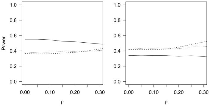
The power for various methods are compared. The higher criticism applied to the decorrelated test statistics is represented by the solid line. The likelihood ratio test is represented by the dotted line. The sequence kernel association test is represented by the dashed line. Power is simulated for each ρ that is a nonnegative multiple of 0·05 and the smoothed results are displayed. Signal sparsity is 5% with β = 0.11 in the left plot with signal sparsity 10% with β = 0.08 in the right plot.

The higher criticism has the highest power in the higher sparsity situations, while the likelihood ratio test and the sequence kernel association test have higher power for lower sparsity. The sequence kernel association test seems to benefit greatly from increased correlation, while the higher criticism loses power as ρ increases, because the transformation U^−1/2Z deflates some of the signal for larger ρ, leading to lower power. Overall, it seems that all three methods can be viable. The higher criticism is a good complement to the other methods, and performs better in the presence of weak correlation among the variants and sparse signals.

5. Data analysis

We apply our p-value computation of the higher criticism to a case-control lung cancer genome-wide association study conducted at the Massachusetts General Hospital, which aims at identifying genes that are associated with the risk of non-small-cell lung cancer. The study consists of a total of 984 cases and 970 controls. We use the higher criticism to test for the association of lung cancer risk and each gene, which consists of multiple genetic variants. We analyze 14396 genes throughout the genome with d = 20 genetic variants per gene on average. 92% of genes have d < 50 genetic variants, with the largest d being 1665.

For each gene, we calculate the marginal test statistics Z_j (j = 1, …, d) for genetic variant j by fitting a logistic regression model of case-control status on the genetic variant j while controlling for age, sex, smoking, and principal components for population stratification (Price et al., 2006). As in Section 3, the marginal test statistics corresponding to the genetic variants within the same gene are decorrelated using the Hall & Jin (2010) approach.

Three of the top most significant genes in this analysis were CHRNA5, MYH10, and CLPTM1L, which have been independently found to be associated with lung cancer in previous studies (Spitz et al., 2008; Zienolddiny et al., 2009; Wang et al., 2012). For the CHRNA5, MYH10, and CLPTM1L genes, the higher criticism p-values are 6·37 × 10⁻⁴, 6·42 × 10⁻⁴, and 1·29 × 10⁻²; the sequence kernel association test p-values are 8·19 × 10⁻⁴, 0·41, and 1·54 × 10⁻⁵; and the likelihood ratio test p-values are 4·92 × 10⁻³, 1·96 × 10⁻³, and 7·05 × 10⁻⁴, respectively.

As observed in the power simulations of Section 3, the higher criticism test and the sequence kernel association test complement each other for these most significant genes. In order to correct for multiple comparisons, the higher criticism can be used for signal identification in a hierarchical fashion on the 14396 p-values (Donoho & Jin, 2008). A threshold is set at the point where the test statistics attain the supremum for the higher criticism and all genes with test statistics more extreme than that threshold are declared to be disease-associated. This procedure controls for the false non-discovery rate (Ahdesmki & Strimmer, 2009). In our case this procedure selected the four most significant genes.

As a clear example of why the asymptotic distribution of the higher criticism can be wildly inaccurate for finite d settings, the asymptotic p-values for CHRNA5, MYH10, and CLPTM1L are 5·97 × 10⁻⁷², 3·83 × 10⁻⁶⁴, and 3·27 × 10⁻¹², respectively. These inaccuracies are amplified in the tails of the distribution which is why the asymptotic p-values differ by so many orders of magnitude from the exact p-values obtained from Theorem 2.

6. Discussion

The proposed analytic method for calculating the p-value of the higher criticism is exact for any arbitrary finite d for normally distributed test statistics. It is computationally fast for the common non-large d settings encountered in gene-level analysis in genome-wide association studies. For non-normally distributed outcomes, such as binary outcomes in case-control studies, accuracy of the proposed calculations depends on the accuracy of the normality approximation of individual marginal test statistics. For large sample sizes, which is often the case in genome-wide association studies, the normality assumption of individual test statistics holds quite well and the proposed p-value calculations for an arbitrary d have high accuracy.

While the vast majority of genes in the genome will have only dozens of genetic variants, there may be a very few large genes with d in the thousands. For these large genes, simulating the null distribution could be less of a computational burden than the analytic p-value calculation given by Theorem 2. Hence a mixture of both techniques could lead to a faster overall analysis of genome-wide association data. For example, Theorem 2 could be used to calculate p-values unless the gene has d > 500 in which case simulation of the null distribution could be used to obtain the p-value. In the presence of correlation, the decorrelation transformation (Hall & Jin, 2010) could dampen the non-null signals when the correlation between some of the marginal test statistics is moderate or strong. It would be of future interest to develop an alternative higher criticism method to account for the correlation more effectively to improve the test power.

Appendix 1. Proof of Lemma 1

Proof

Recall that c(t | h) = h[2d Φ̄ (t){1 − 2 Φ̄ (t)}]^1/2 + 2dΦ̄ (t). By letting t → 0, we see that h ≥ 0 and the p-value in this case is 1. Considering a fixed h > 0, we evaluate the behavior of c(t | h). We have, c(0 | h) = d, lim_t→∞ c(t | h) = 0, and the first derivative is

$$c^{\prime }(t\mid h)=d\varphi (t)\left(\frac{h(4\overline{\mathrm{\Phi }}(t)-1)}{{[2d\overline{\mathrm{\Phi }}(t)\{1-2\overline{\mathrm{\Phi }}(t)\}]}^{1/2}}-2\right).$$

Letting t_max = Φ⁻¹[1 − {1 + d(h² + d) ⁻¹}/4], we can see that c(t | h) is increasing on 0 < t < t_max, achieves its maximum at t_max, and is decreasing on t_max < t < ∞ approaching 0. This along with c(0 | h) = d and c(t | h) being continuous gives the result.

Appendix 2. Proof of Theorem 1

Proof

We need only consider t ≥ t₁ rather than take the intersection over all t > 0. Because c(t | h) > d for 0 < t < t₁, and as S(t) ≤ d, S(t) must be less than c(t | h) for every t ∈ (0, t₁) with probability 1. Therefore

$$\text{pr}\left[\underset{t>0}{\cap }\{S(t)<c(t\mid h)\}\right]=\text{pr}\left[\underset{t\ge t_1}{\cap }\{S(t)<c(t\mid h)\}\right].$$

As S(t) an integer-valued non-increasing function of t, we have for each k in 1, …, d that

$$\underset{t_k<t\le t_{k+1}}{\cap }\{S(t)<c(t\mid h)\}=\{S(t_k)\le d-k\}.$$

Using this and breaking the intersection into its partition

$$\underset{t\ge t_1}{\cap }\{S(t)<c(t\mid h)\}=\underset{k=1}{\overset{d}{\cap }}\underset{t_k<t\le t_{k+1}}{\cap }\{S(t)<c(t\mid h)\},$$

the results follow.

References

- Ahdesmki M, Strimmer K. Feature selection in omics prediction problems using cat scores and false non-discovery rate control. The Annals of Applied Statistics. 2009;4:503–519. [Google Scholar]
- Arias-Castro E, Candès EJ, Plan Y. Global testing under sparse alternatives: ANOVA, multiple comparisons and the higher criticism. The Annals of Statistics. 2011;39:2533–2556. [Google Scholar]
- Donoho D, Jin J. Higher criticism for detecting sparse heterogeneous mixtures. The Annals of Statistics. 2004;34:962–994. [Google Scholar]
- Donoho D, Jin J. Higher criticism thresholding: optimal feature selection when useful features are rare and weak. Proceedings of the National Academy of Sciences. 2008;105(39):14790–14795. doi: 10.1073/pnas.0807471105. [DOI] [PMC free article] [PubMed] [Google Scholar]
- Gaenssler P. In: Empirical Processes. Gupta SS, editor. Vol. 3. Institute of Mathematical Statistics; 1983. pp. 1–11. Lecture Notes-Monograph Series. [Google Scholar]
- Hall P, Jin J. Innovated higher criticism for detecting sparse signals in correlated noise. The Annals of Statistics. 2010;38:1686–1732. [Google Scholar]
- Jaeschke D. The asymptotic distribution of the supremum of the standardized empirical distribution function on subintervals. The Annals of Statistics. 1979;7:108–115. [Google Scholar]
- Price A, Patterson N, Plenge R, Weinblatt M, Shadick N, Reich D. Principal components analysis corrects for stratification in genome-wide association studies. Nature Genetics. 2006;38:904–909. doi: 10.1038/ng1847. [DOI] [PubMed] [Google Scholar]
- Spitz M, Amos C, Dong Q, Lin J, Wu X. The CHRNA5-A3 region on chromosome 15q24-25.1 is a risk factor both for nicotine dependence and for lung cancer. Journal of the National Cancer Institute. 2008;100:1552–1556. doi: 10.1093/jnci/djn363. [DOI] [PMC free article] [PubMed] [Google Scholar]
- Tzeng JY, Zhang D. Haplotype-based association analysis via variance components score test. The American Journal of Human Genetics. 2007;81:927–938. doi: 10.1086/521558. [DOI] [PMC free article] [PubMed] [Google Scholar]
- Wang C, Chien K, Wang C, Liu H, Cheng C, Chang Y, Yu J, Yu C. Quantitative proteomics reveals regulation of KPNA2 and its potential novel cargo proteins in non-small cell lung cancer. Molecular & Cellular Proteomics. 2012;12 doi: 10.1074/mcp.M111.016592. [DOI] [PMC free article] [PubMed] [Google Scholar]
- Wu MC, Lee S, Cai T, Li Y, Boehnke M, Lin X. Rare-variant association testing for sequencing data with the sequence kernel association test. The American Journal of Human Genetics. 2011;89:82–93. doi: 10.1016/j.ajhg.2011.05.029. [DOI] [PMC free article] [PubMed] [Google Scholar]
- Zienolddiny S, Skaug V, Landvik N, Ryberg D, Phillips D, Houlston R, Haugen A. The TERT-CLPTM1L lung cancer susceptibility variant associates with higher DNA adduct formation in the lung. Carcinogenesis. 2009;30:1368–1371. doi: 10.1093/carcin/bgp131. [DOI] [PubMed] [Google Scholar]
Associated Data
This section collects any data citations, data availability statements, or supplementary materials included in this article.