Abstract
The maintenance of genetic diversity in fitness-related traits remains a central topic in evolutionary biology, for example, in the context of sexual selection for genetic benefits. Among the solutions that have been proposed is directional sexual selection for heterozygosity. The importance of such selection is highly debated. However, a critical evaluation requires knowledge of the heritability of heterozygosity, a quantity that is rarely estimated in this context, and often assumed to be zero. This is at least partly the result of the lack of a general framework that allows for its quantitative prediction in small and inbred populations, which are the focus of most empirical studies. Moreover, while current predictors are applicable only to biallelic loci, fitness-relevant loci are often multiallelic, as are the neutral markers typically used to estimate genome-wide heterozygosity. To this end, we first review previous, but little-known, work showing that under most circumstances, heterozygosity at biallelic loci and in the absence of inbreeding is heritable. We then derive the heritability of heterozygosity and the underlying variances for multiple alleles and any inbreeding level. We also show that heterozygosity at multiallelic loci can be highly heritable when allele frequencies are unequal, and that this heritability is reduced by inbreeding. Our quantitative genetic framework can provide new insights into the evolutionary dynamics of heterozygosity in inbred and outbred populations.
Introduction
Fisher's fundamental theorem of natural selection states that the rate of increase in fitness is proportional to the additive genetic variance in fitness (Fisher, 1930, Chapter 2). From this it follows that, if selection is the only evolutionary force and the environment is stable, additive genetic variance in fitness will be depleted (e.g., Charlesworth, 1987), reducing responses to selection. This expected depletion of additive genetic variance in fitness has received most interest in the context of mate choice for genetic benefits, as it is difficult to explain how there remains enough additive genetic variance in fitness to make it worthwhile for females to be choosy. This apparent contradiction has been termed the ‘lek paradox' (Borgia, 1979). A number of solutions to the question of how genetic variance in fitness is maintained have been proposed (reviewed in Kokko et al., 2003), one of which is that genetic diversity is maintained by sexual selection for heterozygosity (Borgia, 1979; Brown, 1997). The importance of such selection is, however, highly debated (Lehmann et al., 2007; Fromhage et al., 2009; Aparicio, 2011), and empirical studies testing for a response to (natural or sexual) selection of heterozygosity at fitness-related loci are lacking.
One important component of a rigorous quantitative genetic framework to study such processes is the heritability of heterozygosity. Theoretical studies have shown that heterozygosity is heritable when allele frequencies are unequal (Borgia, 1979; Mitton et al., 1993; Neff and Pitcher, 2008), and a number of empirical studies have reported parent–offspring correlations in heterozygosity itself (Cothran et al., 1983; Mitton et al., 1993; Richardson et al., 2004; Hoffman et al., 2007; García-Navas et al., 2009; Oh, 2009; Thoß, 2010; Thonhauser et al., 2014), or inferred them from a parent–offspring correlation in inbreeding coefficients (Reid et al., 2006). Although the presence of substantial heritability of heterozygosity has been formally shown for two-allelic loci more than two decades ago (Mitton et al., 1993), this is not well known among evolutionary biologists (e.g., Coulson and Clegg, 2014).
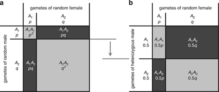
A parent–offspring correlation in heterozygosity may seem surprising, because offspring heterozygosity would appear to be only a function of the genetic similarity of the parents. However, while the genetic similarity of the parents is an important determinant of offspring heterozygosity, under most conditions (i.e., whenever allele frequencies are not equal) offspring heterozygosity also depends on the genetic composition of each parent in isolation. We illustrate this in Figure 1 for a randomly mating population and a single locus with two alleles A1 and A2, with frequencies p and q. As depicted in Figure 1a, the probability of two random individuals having a heterozygous offspring equals 2pq, which if p≠q is <50%. However, the probability of a heterozygous individual and a random individual having a heterozygous offspring is, regardless of the allele frequencies in the population, 50% (Figure 1b). Thus, if p≠q, matings involving a heterozygous individual produce more heterozygous offspring than matings involving two randomly chosen individuals, giving rise to the heritability of heterozygosity. When one allele becomes increasingly rare, the amount by which the proportions of expected heterozygous offspring differ between the two mating types becomes larger, and the heritability of heterozygosity therefore increases when allele frequencies become more unequal. Phrased in another way, heterozygosity is heritable because gametes of heterozygous individuals are on average less likely to share alleles with gametes of a randomly chosen individual from the same population. Thereby, the heritability of heterozygosity does not require fitness differences between homozygotes and heterozygotes, but rather is a neutral process following directly from the principles of Mendelian inheritance.
Figure 1.
Qualitative explanation of heritability of heterozygosity. (a) A situation of random mating where offspring genotypes are produced according to the allele frequencies in the population. At most 50% of the offspring are expected to be heterozygous (dark gray areas). This maximum of 50% heterozygous offspring occurs when allele frequencies are equal (i.e. p=q). (b) A situation where a heterozygous individual mates with a random individual from the population. In this case, half of the offspring are expected to be heterozygous (dark gray areas), regardless of the allele frequencies in the population. Thus, for unequal allele frequencies (i.e. p≠q), matings involving a heterozygous individual produce more heterozygous offspring than random matings. Hence, heterozygosity is heritable when allele frequencies are unequal, or put another way, heterozygosity is heritable because of the presence of rare alleles.
Although we have a quantitative understanding of the heritability of heterozygosity for cases of two alleles and no inbreeding (Mitton et al., 1993), most empirical studies that reported parent–offspring correlations in heterozygosity have used multiallelic genetic (e.g., microsatellite) markers. Additionally, although point mutations in coding DNA usually lead to biallelic single-nucleotide polymorphisms, many fitness-relevant genes will carry multiple mutations leading to multiple haplotypes (e.g., immune genes). Thus, at the scale of a gene rather than a single nucleotide, multiallelic loci are common. Furthermore, the expected heritability of heterozygosity has only been derived for outbred populations. However, many studies measuring heterozygosity are carried out in small and inbred populations, and inbreeding complicates predictions of the heritability by influencing the covariance between parents and offspring (Cockerham and Weir, 1984; de Boer and Hoeschele, 1993; Shaw et al., 1998; Wolak and Keller, 2014).
Here we derive the heritability of heterozygosity for multiple alleles and any inbreeding level. After reviewing the explicit theoretical framework of Mitton et al. (1993) for predicting heritability of heterozygosity at biallelic loci in the absence of inbreeding, we extend their framework to allow for multiple alleles and any degree of inbreeding. We show that multiallelic heterozygosity can be highly heritable when allele frequencies are unequal. We also show how inbreeding affects heritability of heterozygosity. On the whole, this quantitative genetics framework allows for a direct comparison of the observed and the expected heritability of heterozygosity, and thus for the study of the evolutionary dynamics of heterozygosity.
Theoretical framework
The additive and dominance genetic variance of heterozygosity has previously been derived for loci with two alleles by Mitton et al. in Heredity (1993). Here we review these derivations, and subsequently extend them to the multiallelic case. We do this first assuming random mating and a large population size, and then allowing for any level of inbreeding.
Biallelic loci and no inbreeding
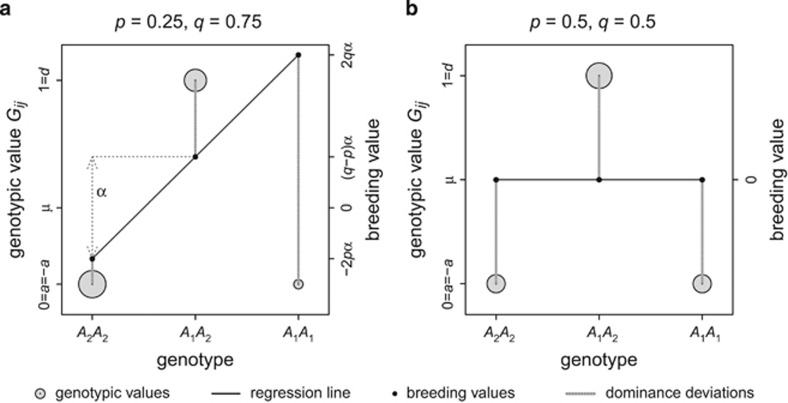
Heterozygosity can be treated as a quantitative genetic trait (Mitton et al., 1993), as is illustrated for the simplest case of one locus with two alleles A1 and A2 and frequencies p and q, respectively, in Figure 2 (following Fisher, 1918; as outlined in Falconer and Mackay, 1996, Chapter 7).
Figure 2.
Derivation of additive and dominance genetic variance of heterozygosity for one locus with two alleles with frequencies p and q (see text for details). Genotypic values Gij of 1 are assigned to heterozygotes and 0 to homozygotes, and thus the mean genotypic value μ of the population equals 2pq. Gray circles represent genotypic values and their surface area represents genotype frequencies. Predicted values of a least-squares regression (black line) weighted by genotype frequencies of Gij on the number of A1 alleles represent breeding values (black dots) and the slope of this regression represents the average effect of allelic substitution α. Variance in breeding values represents the additive genetic variance. Dominance deviations (gray vertical lines) are differences between breeding values and genotypic values Gij, and their variance represents dominance genetic variance. Panel a shows an example of unequal allele frequencies, in which case there exists additive genetic variance in heterozygosity, causing heritability of heterozygosity. Panel b shows the case of equal allele frequencies, leading to no additive genetic variance, but considerable dominance genetic variance.
We first assign a genotypic value Gij of 0 to homozygotes (i.e., allele i=j) and 1 to heterozygotes (i.e., i≠j). Following Falconer and Mackay (1996, Chapter 7), the genotypic values of the two homozygotes (a and −a) are expressed relative to their midpoint, and the deviation of the heterozygote from this midpoint as d, the dominance coefficient. In the case of heterozygosity, a =−a=0 and d=1. The average effect α of substituting allele A2 with A1, given by a+d(q−p) (Falconer and Mackay 1996, p 114), reduces to q−p in the case of heterozygosity. This average effect of allelic substitution equals the slope of a least-squares regression of genotypic values on the number of copies of allele A1, weighted by genotype frequencies. On a scale where the population mean is set to 0, the estimated genotypic values of such a weighted regression represent the breeding values of the corresponding genotypes, and the residuals represent dominance deviations. From this it follows that the breeding values for heterozygosity of the A1A1, A1A2 and A2A2 genotypes are 2q(q−p), (q−p)2 and −2p(q−p), respectively. Note that Lynch and Walsh (1998, Chapter 4) use an alternative formulation of d, namely d=(1+k)a, where k is undefined for a=0.
One definition of additive genetic variance ( ) is the variance in breeding values, which is obtained by squaring the breeding values and summing across genotypes, while weighting by genotype frequencies. This yields
  in the general case (Falconer and Mackay, 1996, Equation (8.3b)), and reduces to
  for heterozygosity (Mitton et al., 1993). Similarly, dominance deviations can be expressed as functions of p, q and d (Falconer and Mackay, 1996, p 118). Because d=1 for heterozygosity, dominance deviations are −2q2 for A1A1, 2pq for A1A2 and −2p2 for A2A2. Summing across the squared dominance deviations and weighting by genotype frequencies yields the dominance genetic variance
  (Falconer and Mackay, 1996, Equation (8.4)), which equals 4p2q2 for heterozygosity (Mitton et al., 1993). Because heterozygosity does not exhibit environmental variance, in the absence of inbreeding (see below), the total variance in heterozygosity is equal to the genetic variance
  , which is equal to the sum of
  and
and  . Thus, narrow-sense heritability of heterozygosity is
  , which equals
  or
or  . Thus, the heritability of heterozygosity can, at least for biallelic loci, be predicted from allele frequencies alone.
Multiallelic loci and no inbreeding
Additive genetic variance
To extend the formulations for biallelic loci (see above) to accommodate loci with n alleles, we follow Lynch and Walsh (1998, pp 71–89) for the case of random mating and infinite population size. In this case, the additive effect of allele i is
 |
with μG being the population mean heterozygosity (see below). Assigning as before genotypic values (Gij) of 0 to homozygotes (i.e., i=j, with i and j representing the two alleles of a diploid individual) and genotypic values of 1 to heterozygotes (i.e., i≠j), this simplifies to
 |
From this it directly follows that rare alleles have larger additive effects on heterozygosity than common alleles.
Under Hardy–Weinberg equilibrium (Hardy, 1908; Weinberg, 1908), the population mean heterozygosity  , with k indicating alleles (Nei, 1987, Equation (8.1)). Substituting this for μG in Equation (1a) yields
 |
We can now substitute Equation (1b) into the general expression for the additive genetic variance (Lynch and Walsh, 1998, Equation (4.23b)),
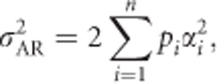 |
where we use subscript R to emphasize that this variance is for a randomly mating and infinitely large population. Using Equation (1b), this yields
 |
Equation (2) shows that, as is the case for biallelic loci, the additive genetic variance of heterozygosity is fully defined by the allele frequencies. This derivation is general regarding the number of alleles and reduces to the equation in Mitton et al. (1993) of  (because (q−p)2=(p−q)2) when applied to a biallelic locus with allele frequencies p and q.
Dominance variance
The dominance deviation δij is the deviation of the genotypic value from the breeding value for each genotype (Figure 2; Lynch and Walsh, 1998, p 73):
If we substitute Equation (1a) for αi and αj, we get
 |
Following Cockerham and Weir (1984), we can calculate the dominance variance for a randomly mating and infinitely large population as
 |
where the subscript R again denotes that this is the variance of an infinitely large and randomly mating population.
Using 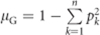 , this yields
 |
Note that summation has to be across all possible values of i and j, and therefore each heterozygous genotype is included twice.
Total genetic variance
Assuming Hardy–Weinberg equilibrium (Hardy, 1908; Weinberg, 1908), we can calculate the total genetic variance of heterozygosity  as the squared deviation of genotypic values from the population mean, weighted by genotype frequencies (Quinn and Keough, 2002, p 10):
 |
Splitting this equation into separate terms giving the contribution of homozygotes (i.e., Gij=0, with i=j) and heterozygotes (Gij=1, with i≠j) yields
 |
We use  (see above) and (0−μG)2=μG2 to get
 |
An alternative, but equivalent approach using Var(X)=E(X2)−E(X)2 (Bolker, 2008, p 118) yields the slightly simpler equation
 |
Thus, rearrangement of Equation (5b) shows that the genetic variance in heterozygosity is a function of mean heterozygosity μG:
Conveniently, we can apply  and use Equations (2) and (5b) to get an alternative equation for the computationally involved Equation (4):
 |
Heritability
For a trait without environmentally induced variation (such as heterozygosity), the broad-sense heritability is one, except in the special case where  . The narrow-sense heritability of heterozygosity can be calculated using Equations (2) and (5b) as
 |
Multiple loci
Without epistasis, measures of genetic variance obtained from several loci can be combined by summing all locus-specific predictions of variance components (Mitton et al., 1993; Falconer and Mackay, 1996, p 129). This means that for the case of heterozygosity, multilocus predictions will behave similarly to the average single-locus prediction, and the extension of the predictions arrived at above to multiple loci is straightforward. However, if there is strong gametic phase disequilibrium, which affects additive and dominance genetic variances and therefore heritability estimates, the extension to multiple loci becomes more complicated (Lynch and Walsh, 1998, p 102) and is beyond the scope of the framework outlined here. At present, it may thus be most practical to prune the data set so that only loci in gametic phase equilibrium remain (Purcell et al., 2007). Identity disequilibrium will be explicitly dealt with in the extensions for inbred populations (Cockerham and Weir, 1984) and will therefore not cause problems for predictions based on multiple loci (see below).
Whereas in the absence of missing data, heterozygosity measures such as the proportion of heterozygous loci among the genotyped loci (i.e., multilocus heterozygosity; Coltman and Slate, 2003) or its standardized equivalent, standardized heterozygosity (Coltman et al., 1999), weight all loci equally, measures such as internal relatedness (Amos et al., 2001) or homozygosity by loci (Aparicio et al., 2006) include some type of weighting according to allele frequencies. For the latter two measures, additivity across loci is therefore not guaranteed. For example, the measure of homozygosity by loci (Aparicio et al., 2006) gives more weight to loci with high mean heterozygosity. Because such loci often tend to have lower heritability of heterozygosity (see below and Figure 6), using homozygosity by loci will lead to an underestimation of the heritability of heterozygosity. Because all four measures of heterozygosity are strongly correlated (Chapman et al., 2009), we therefore recommend the use of multilocus heterozygosity (Coltman and Slate, 2003) or, when a considerable portion of genotypes are missing, standardized heterozygosity (Coltman et al., 1999) as measures for comparing predicted and estimated heritability of heterozygosity.
Inbreeding
Many populations, both captive and natural long-term study populations of vertebrates (Clutton-Brock and Sheldon, 2010), are small and/or fragmented. This often leads to non-negligible levels of inbreeding within populations, either due to genetic drift (under random mating) or due to non-random mating, for example, in selfing organisms or during experimental breeding (Keller and Waller, 2002). The derivations below apply to both types of inbreeding.
In inbreeding populations, the total genetic variance  contains two to four (depending on the type of population; see below) additional genetic (co)variance components (Harris, 1964; Cockerham and Weir, 1984; de Boer and Hoeschele, 1993; Wolak and Keller, 2014). Because these components influence the genetic covariance between parents and offspring in inbred populations, they affect the response to selection (Cockerham and Weir, 1984; Shaw et al., 1998; Kelly, 1999; Kelly and Arathi, 2003; Wolak and Keller, 2014).
Following Cockerham and Weir (1984), but using when applicable the nomenclature of Wolak and Keller (2014), in inbred populations,
 |
All variables in Equation (8) are briefly explained here and will be derived for the case of heterozygosity below. F is Wright's (1969, Chapter 7) individual inbreeding coefficient, which includes effects of non-random mating within populations and genetic drift (Keller and Waller, 2002).  are the additive and dominance genetic variances of the base population, respectively, that is, if the focal population was randomly mating and non-inbred (i.e., infinitely large), and are given by Equations (2) and (6). σADI (called D1 in Cockerham and Weir, 1984) is the covariance between the additive effect of alleles and their homozygous dominance deviations, and
  is the dominance variance due to complete inbreeding. In both cases, the subscript I denotes a component calculated for fully inbred parts of the population. H* is the per-locus inbreeding depression parameter. Finally, (H2−H*) is a measure related to identity disequilibrium (a correlation in heterozygosity across loci; Weir and Cockerham, 1973; David et al., 2007; Szulkin et al., 2010) and therefore only relevant when multiple loci are considered, with H2 being related to H* but summed differently across loci (see below). Here it is assumed that the population is in inbreeding equilibrium, that is, that the level of inbreeding is stable across generations. If this is not the case, this last term may change (Cockerham and Weir, 1984). Note that H2 of Equation (8), used here for consistency with Cockerham and Weir (1984), should not be confused with the broad-sense heritability. Without inbreeding (F=0), Equation (8) reduces to
  , whereas under complete inbreeding (F=1), Equation (8) becomes
  .
.
All terms are needed for large inbred populations (e.g., populations with an individual probability of selfing >0 and <1) for which the mean but not the individual inbreeding coefficients are known. In this case, the last term in Equation (8) (which is always zero if only one locus is considered) accounts for identity disequilibrium because of variance in inbreeding around the mean inbreeding coefficient and may become very large if many loci are considered (Cockerham and Weir, 1984). When variance components are estimated across one or several sub-populations experimentally derived from an infinitely large population and where all individuals have the same known inbreeding coefficient, H* is required but not the last term of Equation (8), because there is no variance in inbreeding coefficients and hence no identity disequilibrium. If inbreeding occurs because of random mating in a small population, the last two terms in Equation (8) are not required (Chevalet and Gillois, 1977). Note that it is only necessary to use the latter approach in small randomly mating populations if allele frequencies are taken from the ancestral population. In cases of random mating where allele frequencies are taken from the current population and loci are in Hardy–Weinberg equilibrium,  .
.
Derivation of additive and dominance variance under inbreeding
With inbreeding, but without unaccounted identity disequilibrium (i.e., when the last term in Equation (8) equals zero, which is the case when there is no variance in inbreeding or when individual inbreeding coefficients are known), Cockerham and Weir (1984) (Equations (1a) and (b)) show that genetic variance can be decomposed into two components, the additive and dominance genetic variance with inbreeding (i.e.,  ), with the subscripted F denoting that these variances refer to a decomposition into only two components (
 ) in an inbred population:
 |
and
 |
For F=0, these equations again reduce to  , whereas for F=1,
  and
and  .
.
Alternatively,  can in principle be derived directly from allele frequencies and additive effects following methods from Kempthorne (1957, p 350) as explained in Supplementary Information 2. However, it should be noted that the derivation by Kempthorne (1957, p 350) is incorrect, leading to an erroneous formula that is also repeated in Lynch and Walsh (1998, Equation (4.24)). See Supplementary Information 2 for a corrected derivation. Falconer (1985) provides an alternative explanation on how to calculate
  .
.
Derivation of other genetic (co)variance components under inbreeding
We will now derive formulae for all remaining genetic (co)variance components in Equation (8) for heterozygosity as a trait, starting from equations in Cockerham and Weir (1984), Shaw et al. (1998), Lynch and Walsh (1998, Chapter 4) and Falconer and Mackay (1996, Chapters 7 and 8).
The covariance σADI (called D1 in Cockerham and Weir, 1984) between the additive effects of alleles and their homozygous dominance deviations can be calculated as
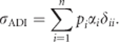 |
For heterozygosity, the dominance deviations of homozygotes δii can be substituted using Equation (3a) and Gii=0, which yields
 |
Using Equation (1a) for αi yields
 |
and subsequently substituting  produces
 |
The dominance variance due to complete inbreeding,  , is given by D2−H*, where
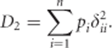 |
For the case of heterozygosity, δii can be substituted for Equation (3b), with Gii=0 and  , which gives
 |
Because  , we use
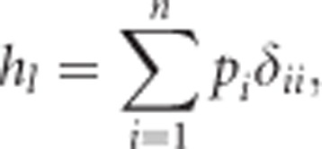 |
where, in the case of heterozygosity, δii can again be substituted for Equation (3b), with Gii=0 and  , to get
 |
Squaring hl yields the squared per-locus inbreeding depression parameter H*
 |
Using Equations (12) and (14), we get for  (called D2* in Cockerham and Weir, 1984)
 |
All components of Equation (8) derived so far can be extended to multiple loci by summing individual-locus values. However, the last term of Equation (8) contains H2, which is derived by summing hl (Equation (13)) across loci, followed by squaring this sum:
 |
If there is only one locus under consideration, H2=H*, and the last term of Equation (8) becomes zero. Furthermore, this last term of Equation (8) is not necessary if individual inbreeding coefficients are known or if there is no variance in inbreeding (de Boer and Hoeschele, 1993; Shaw et al., 1998).
Heritability under inbreeding
Narrow-sense heritability can be defined in multiple ways: As the ratio of additive genetic variance (i.e., the population variance in breeding values) divided by the total phenotypic variance, or as the slope of a regression of mean offspring values on mean parental values (reviewed in Charlesworth, 1987). With inbreeding or gametic phase disequilibrium, equivalence of these definitions is not guaranteed (Charlesworth, 1987).
Animal models, which are commonly used to estimate quantitative genetic parameters in domestic and wild populations, and which are able to simultaneously use all available pedigree information, estimate the heritability as the proportion of phenotypic variance  explained by additive genetic variance for a base population (Henderson, 1984; Kruuk, 2004; Mrode, 2005; Postma, 2006). This base population is assumed to be made up of unrelated individuals, and the individuals with unknown parents in the pedigree are assumed to be a random sample of this base population (Mrode, 2005). Heritability estimated from an animal model thus uses the ratio
  , which for heterozygosity equals
  .
.  must therefore be predicted from Equation (8) by setting F=0, resulting in
  (see also Shaw et al., 1998), yielding a heritability that is independent of inbreeding in the focal population.
To predict the ratio of additive genetic variance to total phenotypic variance in an inbred population, we use heritability defined as  , that is, the proportion of phenotypic variance because of variance in breeding values in an inbred population. For heterozygosity, this equals
  , giving (using Equation (9))
 |
This heritability refers to an inbred population (e.g., Falconer, 1985), but depending on the actual population structure, its relationship with parent–offspring covariance may not be obvious (Nyquist, 1991; Gibson, 1996).
If expected effects of inbreeding are small (see below) or if inbreeding is due to genetic drift and random mating, heritability can be estimated as the slope of a regression of mean offspring phenotype on the mean phenotype of the two parents, for example, following the procedure in Lynch and Walsh (1998, Chapter 17) while weighting for family size following Kempthorne and Tandon (1953). Although this method overestimates heritabilities in the presence of maternal, paternal or common environmental effects, none of these affect heterozygosity, making offspring–parent regressions a good way to estimate heritability of heterozygosity. Because correlations in inbreeding level between parents and offspring may be common in small populations (Reid et al., 2006; Reid and Keller, 2010), the negative effect of inbreeding on heterozygosity should also be considered (Wolak and Keller, 2014). This can be done by using the variation in heterozygosity not explained by inbreeding coefficient (i.e., the residuals of a regression of heterozygosity on F), for example, by including F as a covariate in the animal model (Wolak and Keller, 2014).
Results
Outbred populations
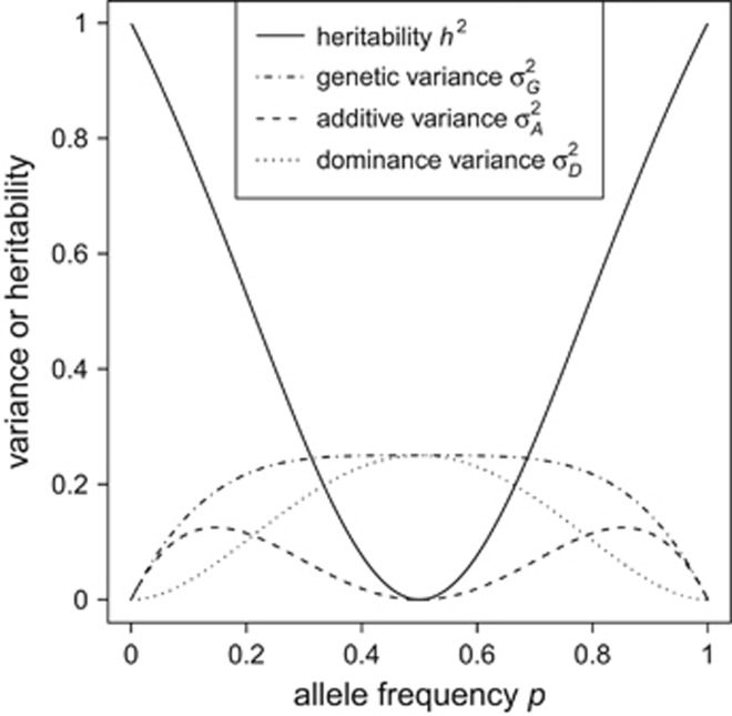
Our theoretical framework allows for prediction of heritability of heterozygosity for loci with multiple alleles and any level of inbreeding, solely as a function of allele frequencies and inbreeding. Such predictions have previously been derived for loci with two alleles and no inbreeding (Mitton et al., 1993). In line with these previous results, we show that for biallelic loci the heritability of heterozygosity increases with increasingly unequal allele frequencies, and that it approaches one as an allele approaches fixation (Figure 3). Note that h2 is not defined when one allele is fixed, because in that case there is no genetic variation. Hence, heritability of heterozygosity is maximal when additive and total genetic variances become minimal (i.e., with highly unequal allele frequencies). Thus, at these limits, heritability of heterozygosity may be of limited biological relevance because there is very little variation in heterozygosity. However, at moderately unequal allele frequencies, both additive and total genetic variance and heritability of heterozygosity are high.
Figure 3.
Expected genetic variance components and heritability of heterozygosity for a locus with two alleles. Note that additive genetic variance is maximal at allele frequencies of  (which is at p≈0.146 and ≈0.854), whereas heritability approaches maximal values at highly unequal allele frequencies.
Unlike h2, additive genetic variance of heterozygosity is maximal at allele frequencies  and
and  (revealed by setting the first derivative of the two-allele version of Equation (2) to zero; these maxima are approximately at p≈0.146 and ≈0.854) and zero at allele frequencies P=0, 0.5 and 1 (Figure 3). Thus, this represents a case of pure overdominance (Crow and Kimura, 1970, Table 4.1.1; Falconer and Mackay, 1996, Figure 8.1c).
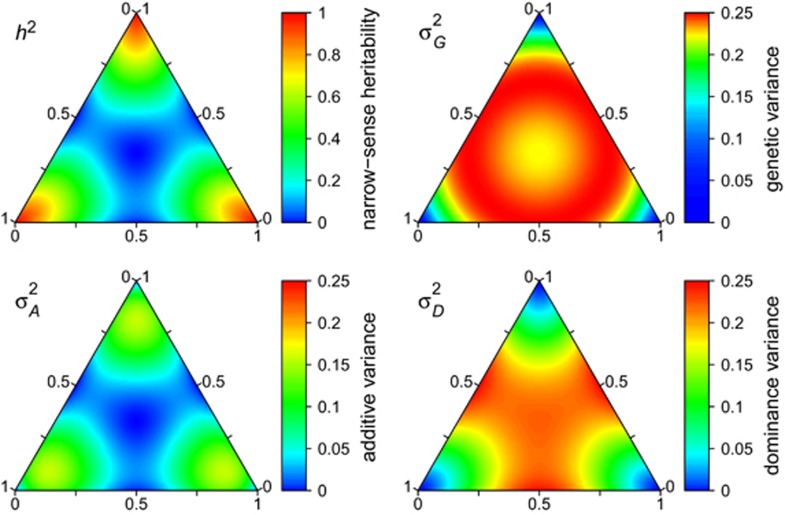
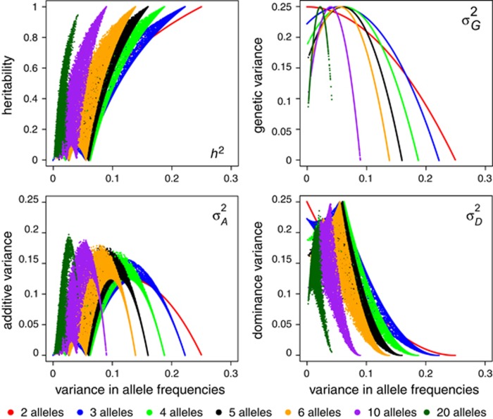
A similar pattern emerges when loci with more than two alleles are considered. For the case of three alleles, narrow-sense heritability of heterozygosity reaches its maximum when one allele is nearly fixed, whereas heterozygosity is not heritable when all three alleles have equal frequencies (Figure 4). As is the case for two alleles, additive genetic variance is maximal when all three alleles are present at non-zero and unequal frequencies. For the case of more than three alleles, we can use the variance in allele frequencies for visualization of the dependence of the genetic variance components on the (variance in) allele frequencies. To illustrate this, we randomly sampled allele frequencies from a Dirichlet distribution. We set the shape parameter α to 0.15 to ensure sampling of a wide range of allele frequencies. We plotted heterozygosity and genetic variance components against variance in allele frequencies for 2 to 6, 10 and 20 alleles at a locus (Figure 5). As shown by Equations (S1.2) and (S1.3) (Supplementary Information 1),  is a function of only the variance in allele frequencies and the number of alleles at the locus, whereas
  ,
,  and h2 are functions of variance in allele frequencies, number of alleles at the locus and actual allele frequencies. Figure 5 also shows that the heritability of heterozygosity increases with increasing variance in allele frequencies (i.e., with increasingly unequal allele frequencies), whereas whenever there are more than two alleles,
  ,
,  and
and  are maximal at intermediate variances in allele frequencies.
Figure 4.
Expected genetic variance components and heritability of heterozygosity for a locus with three alleles in a randomly mating, infinitely large population are shown in simplex plots. Along each side of the triangle, one allele has a frequency of 0%, which increases with distance away from the triangle side until reaching a frequency of 100% at the opposite corner. Colors indicate the values of heritability, total genetic, additive and dominance genetic variance, respectively. Note that the range of values is different for heritability than for the three genetic variance components. Note that the color key is different for genetic variance to allow for better visibility of patterns.
Figure 5.
Relationship between variance in allele frequencies and heritability or genetic variance components of heterozygosity for different numbers of alleles. Note that the relationships are similar in shape for different numbers of alleles, but high variance in allele frequencies can only be reached when few alleles are present, leading to compressed curves for higher numbers of alleles. Although theoretically possible, many variances in allele frequencies shown here are unlikely or impossible in reasonably sized populations (e.g., <1000 individuals) because they may require some extremely low allele frequencies.
An alternative statistic to visualize the dependence of  ,
,  ,
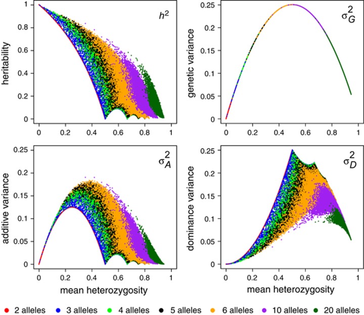
,  and h2 on allele frequencies is provided by relating them to mean heterozygosity (Figure 6). Total genetic variance in heterozygosity (
 ) is a quadratic function of mean heterozygosity only (Equation (S1.5) in Supplementary Information 1). Taking the first derivative of Equation (S1.5) and setting it to zero (or looking at Figure 6) shows that total genetic variance in heterozygosity is maximal when mean heterozygosity μG=0.5.
  ,
,  and h2 are only partly predicted by mean heterozygosity, and information about actual allele frequencies is needed for their accurate prediction. Figure 6 shows that additive and dominance genetic variance in heterozygosity are maximal when mean heterozygosity is intermediate, with the exact location of the maximum shifting with the number of alleles present. Heritability of heterozygosity decreases with increasing mean heterozygosity.
Figure 6.
Relationship between mean heterozygosity and heritability or genetic variance components of heterozygosity for different numbers of alleles. Although theoretically possible, many data points shown here are unlikely or impossible in reasonably sized populations (e.g. <1000 individuals) because they may require some extremely low allele frequencies.
In summary, we have shown that for any number of alleles in an outbred population, heritability of heterozygosity is highest for highly unequal allele frequencies, whereas additive genetic variance in heterozygosity is highest for moderately unequal allele frequencies.
Inbred populations
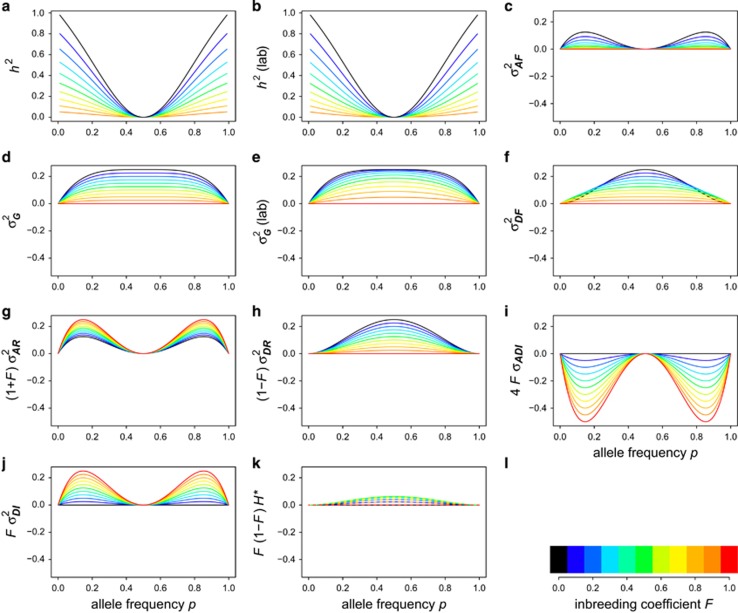
The effects of inbreeding on the heritability of heterozygosity depend slightly on the type of population considered, but inbreeding always reduces the heritability of heterozygosity (Figures 7a and b). Heritability in small and randomly mating populations (where the last two terms of Equation (8) are not required) is slightly higher than in one or several sub-populations derived from an infinitely large population where all individuals have the same known inbreeding coefficient (where only the last term of Equation (8) is not required). For F=1, heritability of heterozygosity approaches 0, but is not defined because in that case all individuals are homozygous, and there is no genetic variance in heterozygosity.
Figure 7.
Plots of all genetic (co)variance components and heritability of heterozygosity under inbreeding. Values for a set of inbreeding coefficients are colored according to (l). (a and d) A randomly mating population with inbreeding because of genetic drift. (b and e) Experimental populations where one or several lines are inbred to a known and identical degree and descending from an infinitely large randomly mating population. These distinctions are not necessary for the other panels. Heritability (h2) of heterozygosity approaches 0, but is not defined for complete inbreeding (F=1) because then there is no genetic variance for heterozygosity as all individuals are completely homozygous (a and b). Genetic variance in heterozygosity (d and e) decreases with inbreeding. When genetic variance is partitioned into two components only (Equations (9) and (10)), both additive (c) and dominance (f) genetic variance decrease with inbreeding. When genetic variance is partitioned into five or six components (Equation (8)), the contribution from additive genetic variance because of random mating (g) increases with inbreeding, whereas the corresponding dominance variance (h) decreases. The covariance between the additive effect of alleles and their homozygous dominance deviations (i) becomes increasingly negative with inbreeding, whereas the dominance variance because of inbreeding (j) becomes increasingly positive. The inbreeding depression effect (k) is maximal for F=0.5 and 0 for F=0 and F=1, which means that some curves fall on top of each other (thus they are dashed).
Because inbreeding reduces heterozygosity, total genetic variance in heterozygosity is lowered by inbreeding (Figures 7d and e). Under complete inbreeding, all individuals are homozygous and there is no genetic variance in heterozygosity. When total genetic variance  of the inbred population is partitioned into only two components, the additive genetic variance in the inbred population (
 ; Figure 7c) becomes zero with complete inbreeding, as does the corresponding dominance variance (
 ; Figure 7f). As is the case for any quantitative trait, the contribution of random-mating additive genetic variance (
 ; Figure 7g) increases with stronger inbreeding, and the contribution from random-mating dominance variance (
 , Figure 7h) decreases.
Inbreeding dominance variance ( ; Figure 7j) increases with inbreeding for moderately unequal allele frequencies, and at complete inbreeding it behaves similarly to the contribution of random-mating additive genetic variance (
 ; Figure 7g). The covariance between additive effects and homozygous dominance deviations (4FσADI; Figure 7i) is always negative under inbreeding, and is strongest when inbreeding is high and allele frequencies are moderately unequal. As for any trait,
  and
and  are 0 if alleles are equally frequent (Cockerham and Weir, 1984). The inbreeding depression parameter (F(1−F)H* Figure 7k) is 0 for
  or F=1 and reaches its maximum at F=0.5 and equal allele frequencies.
To sum up, we showed how inbreeding affects heritability of heterozygosity in randomly mating populations and in populations where all individuals are experimentally inbred to the same level. In these types of populations, the results hold for any number of loci in gametic phase equilibrium. In populations at equilibrium with unknown individual inbreeding coefficients but known mean inbreeding level (e.g., because only the average selfing rate is known), identity disequilibrium leads to low heritability of heterozygosity when many loci are considered.
Discussion
The fact that heterozygosity can be heritable has been shown more than two decades ago, at least in the case of biallelic loci in outbred populations (Mitton et al., 1993). However, as this is generally not well known, we first reviewed this seminal work. Subsequently, we provided a quantitative genetic framework for the prediction of genetic (co)variance components and heritability of heterozygosity, which allows for any number of multiallelic loci and inbred populations. This provides a useful tool for explicit theoretical and empirical investigations of the importance of selection of heterozygosity for the maintenance of genetic variation in fitness. Indeed, irrespective of the conditions under which selection of heterozygosity might or might not occur, heritability of heterozygosity is an essential requirement for an evolutionary response. The quantitative genetic framework outlined here can be applied to (multiallelic) markers that have fitness effects themselves or to loci that are in linkage disequilibrium with loci that influence fitness (Slatkin, 1995). In addition, heritability of heterozygosity provides an alternative, biologically intuitive explanation for why the dominance coefficient d contributes to additive genetic variance of any trait whenever allele frequencies are unequal (Nietlisbach and Hadfield, 2015).
Whereas heritability of heterozygosity can be calculated for any type of genetic locus, an evolutionary response is not necessarily expected. In particular, allele frequencies at neutral marker loci are not expected to change when they are not linked to loci that are under selection, even if marker heterozygosity correlates with fitness (‘apparent selection' Charlesworth, 1991). In other words, heterozygosity–fitness correlations are not evidence of selection at the marker loci under study (Szulkin et al., 2010). However, when applied to loci that influence fitness, or to loci linked to them, our framework will be useful to evaluate the possibility of an evolutionary response to selection of heterozygosity. Also, the expected response to selection, as predicted from the product of heritability and selection differential (i.e., the breeder's equation), will often deviate from the observed response, for example, if there is no additive genetic covariance between trait and fitness (Merilä et al., 2001; Morrissey et al., 2010, 2012).
Heritability of heterozygosity is highest for highly unequal allele frequencies and is reduced by inbreeding. Reductions in heritability with increasing inbreeding are typical for traits determined by additive gene action. However, with dominance effects, changes in heritability are difficult to predict and can go in any direction (Falconer and Mackay, 1996, p 266), as has been shown experimentally for various traits other than heterozygosity (e.g., Wade et al., 1996; Kristensen et al., 2005). Our framework can be used to assess how strong the effects of inbreeding are on the heritability of heterozygosity in a focal population. This is useful, because empirical estimation of all genetic (co)variance components relevant under inbreeding is very challenging (Wolak and Keller, 2014). Because empirical quantification may often be difficult or impossible, being able to predict these (co)variance components for given allele frequencies and a certain level of inbreeding is of practical relevance. In addition, this framework offers a way to describe the amount of (additive and total genetic) variance in heterozygosity introduced by inbreeding.
Although evaluating the conditions under which heterozygosity may be selected for is beyond the scope of this article, selection for heterozygosity is possible at loci displaying heterozygote advantage (Lehmann et al., 2007; Fromhage et al., 2009). Among the few known loci showing indications for a heterozygote advantage is the major histocompatibility complex (or human leukocyte antigen system in humans), where heterozygous individuals are more resistant against pathogens (reviewed in Hedrick, 2012). However, because most rare alleles occur in heterozygous form (Halliburton, 2004, p 78), it is often not possible to distinguish heterozygote advantage from selection for rare alleles (Spurgin and Richardson, 2010). Nevertheless, even if heterozygote advantage seems to be rare in nature, just a few overdominant loci would have a larger effect compared with many loci with directional dominance (Crow, 1952, p 291). Additionally, there may be a role for pseudo-overdominance (Charlesworth and Willis, 2009) (sometimes called associative overdominance; Frydenberg, 1963; Lynch and Walsh, 1998, p 288) and fluctuating selection (Charlesworth, 1988) in generating selection for heterozygosity.
Conclusion
We have shown for multiallelic loci and for populations with inbreeding that the degree to which heterozygosity is heritable is a function of only allele frequencies and inbreeding coefficients, and that this heritability can be very high under unequal allele frequencies and little inbreeding. In fact, heritability of heterozygosity easily reaches levels as high as those for life-history traits in wild populations (Postma, 2014). Because allele frequencies in natural populations are usually unequal (e.g., Chakraborty et al., 1980; Whittam, 1981; Burns and Zink, 1990), the heritability of heterozygosity is likely often greater than zero. Our theoretical framework provided here enables explicit prediction of heritability of heterozygosity for many situations, including for loci with multiple alleles (e.g., immune genes, haplotypes of multiple single-nucleotide polymorphisms corresponding to functional genes or microsatellites) and for inbred populations. This framework will thus help to critically evaluate the evolutionary dynamics of heterozygosity in natural or laboratory populations.
Data archiving
There are no data to archive.
Acknowledgments
We thank Philipp Becker, Timothée Bonnet, Patrice David, Jarrod Hadfield, Andri Manser, Michael Morrissey, Stefanie Muff, Jon Slate and anonymous reviewers for interesting discussions and helpful comments and suggestions on earlier versions of the manuscript. John Kelly provided insightful advice on variance components under inbreeding. This work was funded in part by a grant of the Swiss National Science Foundation to LFK (Grant 31003A-116794).
The authors declare no conflict of interest.
Footnotes
Supplementary Information accompanies this paper on Heredity website (http://www.nature.com/hdy)
Supplementary Material
References
- Amos W, Wilmer JW, Fullard K, Burg TM, Croxall JP, Bloch D, Coulson T. (2001). The influence of parental relatedness on reproductive success. Proc R Soc Ser B 268: 2021–2027. [DOI] [PMC free article] [PubMed] [Google Scholar]
- Aparicio JM. (2011). The paradox of the resolution of the lek paradox based on mate choice for heterozygosity. Anim Behav 81: 1271–1279. [Google Scholar]
- Aparicio JM, Ortego J, Cordero PJ. (2006). What should we weigh to estimate heterozygosity, alleles or loci? Mol Ecol 15: 4659–4665. [DOI] [PubMed] [Google Scholar]
- Bolker BM. (2008) Ecological Models and Data in R. Princeton University Press: Princeton, NJ, USA. [Google Scholar]
- Borgia G. (1979) Sexual selection and the evolution of mating systems. In: Blum MS, Blum NA (eds). Sexual Selection and Reproductive Competition in Insects. Academic Press: New York, NY, USA. [Google Scholar]
- Brown JL. (1997). A theory of mate choice based on heterozygosity. Behav Ecol 8: 60–65. [Google Scholar]
- Burns KJ, Zink RM. (1990). Temporal and geographic homogeneity of gene frequencies in the Fox sparrow (Passerella iliaca. Auk 107: 421–425. [Google Scholar]
- Chakraborty R, Fuerst PA, Nei M. (1980). Statistical studies on protein polymorphism in natural populations. III. Distribution of allele frequencies and the number of alleles per locus. Genetics 94: 1039–1063. [DOI] [PMC free article] [PubMed] [Google Scholar]
- Chapman JR, Nakagawa S, Coltman DW, Slate J, Sheldon BC. (2009). A quantitative review of heterozygosity–fitness correlations in animal populations. Mol Ecol 18: 2746–2765. [DOI] [PubMed] [Google Scholar]
- Charlesworth B. (1988). The evolution of mate choice in a fluctuating environment. J Theor Biol 130: 191–204. [DOI] [PubMed] [Google Scholar]
- Charlesworth B. (1987) The heritability of fitness. In: Bradbury JW, Andersson MB (eds). Sexual Selection: Testing the Alternatives. Wiley: Chichester, UK, pp 21–40. [Google Scholar]
- Charlesworth D. (1991). The apparent selection on neutral marker loci in partially inbreeding populations. Genet Res 57: 159–175. [Google Scholar]
- Charlesworth D, Willis JH. (2009). The genetics of inbreeding depression. Nat Rev Genet 10: 783–796. [DOI] [PubMed] [Google Scholar]
- Chevalet C, Gillois M. (1977) Estimation of genotypic variance components with dominance in small consanguineous populations. In: Pollak E, Kempthorne O, Bailey TBJ (eds). Proceedings of the International Conference on Quantitative Genetics. Iowa State University Press: Ames, IA, USA, pp 271–296. [Google Scholar]
- Clutton-Brock T, Sheldon BC. (2010). Individuals and populations: the role of long-term, individual-based studies of animals in ecology and evolutionary biology. Trends Ecol Evol 25: 562–573. [DOI] [PubMed] [Google Scholar]
- Cockerham CC, Weir BS. (1984). Covariances of relatives stemming from a population undergoing mixed self and random mating. Biometrics 40: 157–164. [PubMed] [Google Scholar]
- Coltman DW, Pilkington JG, Smith JA, Pemberton JM. (1999). Parasite-mediated selection against inbred Soay sheep in a free-living, island population. Evolution 53: 1259–1267. [DOI] [PubMed] [Google Scholar]
- Coltman DW, Slate J. (2003). Microsatellite measures of inbreeding: a meta-analysis. Evolution 57: 971–983. [DOI] [PubMed] [Google Scholar]
- Cothran EG, Chesser RK, Smith MH, Johns PE. (1983). Influences of genetic variability and maternal factors on fetal growth in white-tailed deer. Evolution 37: 282–291. [DOI] [PubMed] [Google Scholar]
- Coulson T, Clegg S. (2014). Fur seals signal their own decline. Nature 511: 414–415. [DOI] [PubMed] [Google Scholar]
- Crow JF. (1952) Dominance and overdominance. In: Gowen JW (ed). Heterosis. Iowa State College Press: Ames, IA, USA, pp 282–297. [Google Scholar]
- Crow JF, Kimura M. (1970) An Introduction to Population Genetics Theory. The Blackburn Press: Caldwell, NJ, USA. [Google Scholar]
- David P, Pujol B, Viard F, Castella V, Goudet J. (2007). Reliable selfing rate estimates from imperfect population genetic data. Mol Ecol 16: 2474–2487. [DOI] [PubMed] [Google Scholar]
- De Boer IJM, Hoeschele I. (1993). Genetic evaluation methods for populations with dominance and inbreeding. Theor Appl Genet 86: 245–258. [DOI] [PubMed] [Google Scholar]
- Falconer DS. (1985). A note on Fisher's 'average effect' and 'average excess'. Genet Res 46: 337–347. [DOI] [PubMed] [Google Scholar]
- Falconer DS, Mackay TFC. (1996) Introduction to Quantitative Genetics, 4th edn. Pearson Education Limited: Harlow, UK. [Google Scholar]
- Fisher RA. (1918). The correlation between relatives on the supposition of Mendelian inheritance. Earth Environ Sci Trans R Soc 52: 399–433. [Google Scholar]
- Fisher RA. (1930) The Genetical Theory of Natural Selection. Clarendon Press: Oxford, UK. [Google Scholar]
- Fromhage L, Kokko H, Reid JM. (2009). Evolution of mate choice for genome-wide heterozygosity. Evolution 63: 684–694. [DOI] [PubMed] [Google Scholar]
- Frydenberg O. (1963). Population studies of a lethal mutant in Drosophila melanogaster. I. Behaviour in populations with discrete generations. Hereditas 50: 89–116. [Google Scholar]
- García-Navas V, Ortego J, Sanz JJ. (2009). Heterozygosity-based assortative mating in blue tits (Cyanistes caeruleus: implications for the evolution of mate choice. Proc R Soc Ser B 276: 2931–2940. [DOI] [PMC free article] [PubMed] [Google Scholar]
- Gibson PT. (1996). Correcting for inbreeding in parent–offspring regression estimates of heritability with non-additive and genotype × environment effects present. Crop Sci 36: 594–600. [Google Scholar]
- Halliburton R. (2004) Introduction to Population Genetics. Pearson Prentice-Hall: Upper Saddle River, NJ, USA. [Google Scholar]
- Hardy GH. (1908). Mendelian proportions in a mixed population. Science 28: 49–50. [DOI] [PubMed] [Google Scholar]
- Harris DL. (1964). Genotypic covariances between inbred relatives. Genetics 50: 1319–1348. [DOI] [PMC free article] [PubMed] [Google Scholar]
- Hedrick PW. (2012). What is the evidence for heterozygote advantage selection? Trends Ecol Evol 27: 698–704. [DOI] [PubMed] [Google Scholar]
- Henderson CR. (1984) Applications of Linear Models in Animal Breeding Models. University of Guelph Press: Guelph, ON, Canada. [Google Scholar]
- Hoffman JI, Forcada J, Trathan PN, Amos W. (2007). Female fur seals show active choice for males that are heterozygous and unrelated. Nature 445: 912–914. [DOI] [PubMed] [Google Scholar]
- Keller LF, Waller DM. (2002). Inbreeding effects in wild populations. Trends Ecol Evol 17: 230–241. [Google Scholar]
- Kelly JK. (1999). Response to selection in partially self-fertilizing populations. I. Selection on a single trait. Evolution 53: 336–349. [DOI] [PubMed] [Google Scholar]
- Kelly JK, Arathi HS. (2003). Inbreeding and the genetic variance in floral traits of Mimulus guttatus. Heredity 90: 77–83. [DOI] [PubMed] [Google Scholar]
- Kempthorne O. (1957) An Introduction to Genetic Statistics. Wiley: New York, NY, USA. [Google Scholar]
- Kempthorne O, Tandon OB. (1953). The estimation of heritability by regression of offspring on parent. Biometrics 9: 90–100. [Google Scholar]
- Kokko H, Brooks R, Jennions MD, Morley J. (2003). The evolution of mate choice and mating biases. Proc R Soc Ser B 270: 653–664. [DOI] [PMC free article] [PubMed] [Google Scholar]
- Kristensen TN, Sørensen AC, Sorensen D, Pedersen KS, Sørensen JG, Loeschcke V. (2005). A test of quantitative genetic theory using Drosophila—effects of inbreeding and rate of inbreeding on heritabilities and variance components. J Evol Biol 18: 763–770. [DOI] [PubMed] [Google Scholar]
- Kruuk LEB. (2004). Estimating genetic parameters in natural populations using the 'animal model'. Philos Trans R Soc Lond Ser B 359: 873–890. [DOI] [PMC free article] [PubMed] [Google Scholar]
- Lehmann L, Keller LF, Kokko H. (2007). Mate choice evolution, dominance effects, and the maintenance of genetic variation. J Theor Biol 244: 282–295. [DOI] [PubMed] [Google Scholar]
- Lynch M, Walsh B. (1998) Genetics and Analysis of Quantitative Traits. Sinauer Associates: Sunderland, MA, USA. [Google Scholar]
- Merilä J, Sheldon BC, Kruuk LEB. (2001). Explaining stasis: microevolutionary studies in natural populations. Genetica 112: 199–222. [PubMed] [Google Scholar]
- Mitton JB, Schuster WSF, Cothran EG, Defries JC. (1993). Correlation between the individual heterozygosity of parents and their offspring. Heredity 71: 59–63. [DOI] [PubMed] [Google Scholar]
- Morrissey MB, Kruuk LEB, Wilson AJ. (2010). The danger of applying the breeder's equation in observational studies of natural populations. J Evol Biol 23: 2277–2288. [DOI] [PubMed] [Google Scholar]
- Morrissey MB, Parker DJ, Korsten P, Pemberton JM, Kruuk LEB, Wilson AJ. (2012). The prediction of adaptive evolution: empirical application of the secondary theorem of selection and comparison to the breeder's equation. Evolution 66: 2399–2410. [DOI] [PubMed] [Google Scholar]
- Mrode RA. (2005) Linear Models for the Prediction of Animal Breeding Values, 2nd edn. CABI Publishing: Wallingford, UK. [Google Scholar]
- Neff BD, Pitcher TE. (2008). Mate choice for non-additive genetic benefits: a resolution to the lek paradox. J Theor Biol 254: 147–155. [DOI] [PubMed] [Google Scholar]
- Nei M. (1987) Molecular Evolutionary Genetics. Columbia University Press: New York, NY, USA. [Google Scholar]
- Nietlisbach P, Hadfield JD. (2015). Heritability of heterozygosity offers a new way of understanding why dominant gene action contributes to additive genetic variance. Evolution; e-pub ahead of print 23 June 2015; doi:10.1111/evo.12704. [DOI] [PubMed]
- Nyquist WE. (1991). Estimation of heritability and prediction of selection response in plant populations. CRC Crit Rev Plant Sci 10: 235–322. [Google Scholar]
- Oh KP. (2009). Evolutionary dynamics of sexual traits: demographic, genetic, and behavioral contingencies. PhD thesis. University of Arizona, Tucson, AZ, USA.
- Postma E. (2014) Four decades of estimating heritabilities in wild vertebrate populations: improved methods, more data, better estimates? In: Charmantier A, Garant D, Kruuk LEB (eds). Quantitative Genetics in the Wild. Oxford University Press: Oxford, UK, pp 16–33. [Google Scholar]
- Postma E. (2006). Implications of the difference between true and predicted breeding values for the study of natural selection and micro-evolution. J Evol Biol 19: 309–320. [DOI] [PubMed] [Google Scholar]
- Purcell S, Neale B, Todd-Brown K, Thomas L, Ferreira MA, Bender D et al. (2007). PLINK: a tool set for whole-genome association and population-based linkage analyses. Am J Hum Genet 81: 559–575. [DOI] [PMC free article] [PubMed] [Google Scholar]
- Quinn GP, Keough MJ. (2002) Experimental Design and Data Analysis for Biologists. University Press: Cambridge, UK. [Google Scholar]
- Reid JM, Arcese P, Keller LF. (2006). Intrinsic parent–offspring correlation in inbreeding level in a song sparrow (Melospiza melodia population open to immigration. Am Nat 168: 1–13. [DOI] [PubMed] [Google Scholar]
- Reid JM, Keller LF. (2010). Correlated inbreeding among relatives: occurrence, magnitude, and implications. Evolution 64: 973–985. [DOI] [PubMed] [Google Scholar]
- Richardson D S, Komdeur J, Burke T. (2004). Inbreeding in the Seychelles warbler: environment-dependent maternal effects. Evolution 58: 2037–2048. [DOI] [PubMed] [Google Scholar]
- Shaw RG, Byers DL, Shaw FH. (1998). Genetic components of variation in Nemophila menziesii undergoing inbreeding: morphology and flowering time. Genetics 150: 1649–1661. [DOI] [PMC free article] [PubMed] [Google Scholar]
- Slatkin M. (1995). Hitchhiking and associative overdominance at a microsatellite locus. Mol Biol Evol 12: 473–480. [DOI] [PubMed] [Google Scholar]
- Spurgin LG, Richardson DS. (2010). How pathogens drive genetic diversity: MHC, mechanisms and misunderstandings. Proc Biol Sci 277: 979–988. [DOI] [PMC free article] [PubMed] [Google Scholar]
- Szulkin M, Bierne N, David P. (2010). Heterozygosity–fitness correlations: a time for reappraisal. Evolution 64: 1202–1217. [DOI] [PubMed] [Google Scholar]
- Thonhauser KE, Thoß M, Musolf K, Klaus T, Penn DJ. (2014). Multiple paternity in wild house mice (Mus musculus musculus: effects on offspring genetic diversity and body mass. Ecol Evol 4: 200–209. [DOI] [PMC free article] [PubMed] [Google Scholar]
- Thoß M. (2010). Sexual selection and heterozygosity in wild house mice (Mus musculus musculus. PhD thesis, Universität Wien, Vienna, Austria.
- Wade MJ, Shuster S M, Stevens L. (1996). Inbreeding: its effect on response to selection for pupal weight and the heritable variance in fitness in the flour beetle, Tribolium castaneum. Evolution 50: 723–733. [DOI] [PubMed] [Google Scholar]
- Weinberg W. (1908). Über den Nachweis der Vererbung beim Menschen. Jahreshefte des Vereins für vaterländische Naturkunde in Württemberg 64: 369–382. [Google Scholar]
- Weir BS, Cockerham CC. (1973). Mixed self and random mating at two loci. Genet Res 21: 247–262. [DOI] [PubMed] [Google Scholar]
- Whittam TS. (1981). Variation in gene frequencies in rodent populations: the roles of selective and nonselective evolutionary forces. PhD thesis. University of Arizona, Tucson, AZ, USA.
- Wolak ME, Keller LF. (2014) Dominance genetic variance and inbreeding in natural populations. In: Charmantier A, Garant D, Kruuk LEB (eds). Quantitative Genetics in the Wild. Oxford University Press: Oxford, UK, pp 104–127. [Google Scholar]
- Wright S. (1969) Evolution and the genetics of populations. Volume 2: the theory of gene frequencies. The University of Chicago Press: Chicago, IL, USA. [Google Scholar]
Associated Data
This section collects any data citations, data availability statements, or supplementary materials included in this article.


