A Comparison of the β-Substitution Method and a Bayesian Method for Analyzing Left-Censored Data

Abstract

Classical statistical methods for analyzing exposure data with values below the detection limits are well described in the occupational hygiene literature, but an evaluation of a Bayesian approach for handling such data is currently lacking. Here, we first describe a Bayesian framework for analyzing censored data. We then present the results of a simulation study conducted to compare the β-substitution method with a Bayesian method for exposure datasets drawn from lognormal distributions and mixed lognormal distributions with varying sample sizes, geometric standard deviations (GSDs), and censoring for single and multiple limits of detection. For each set of factors, estimates for the arithmetic mean (AM), geometric mean, GSD, and the 95th percentile (X_0.95) of the exposure distribution were obtained. We evaluated the performance of each method using relative bias, the root mean squared error (rMSE), and coverage (the proportion of the computed 95% uncertainty intervals containing the true value). The Bayesian method using non-informative priors and the β-substitution method were generally comparable in bias and rMSE when estimating the AM and GM. For the GSD and the 95th percentile, the Bayesian method with non-informative priors was more biased and had a higher rMSE than the β-substitution method, but use of more informative priors generally improved the Bayesian method’s performance, making both the bias and the rMSE more comparable to the β-substitution method. An advantage of the Bayesian method is that it provided estimates of uncertainty for these parameters of interest and good coverage, whereas the β-substitution method only provided estimates of uncertainty for the AM, and coverage was not as consistent. Selection of one or the other method depends on the needs of the practitioner, the availability of prior information, and the distribution characteristics of the measurement data. We suggest the use of Bayesian methods if the practitioner has the computational resources and prior information, as the method would generally provide accurate estimates and also provides the distributions of all of the parameters, which could be useful for making decisions in some applications.

INTRODUCTION

In investigating possible detrimental health effects at air concentrations below established exposure limits, the need to incorporate data below the limits of detection (LOD) of the reporting analytic laboratory in data analysis becomes an important part of the exposure assessment strategy. Analysis of this type of censored data (type I left-censoring) requires a statistical approach that not only accounts for the detection limits but also accurately estimates the exposure distributional parameters. Such parameters include the arithmetic mean (AM), which is often used for occupational epidemiological studies (Rappaport, 1991), and the geometric mean (GM), the geometric standard deviation (GSD), and the 95th percentile (X_0.95) for exposure management purposes. Traditionally, point estimates have been used by occupational hygienists for evaluating compliance with regulatory or health-based exposure limits. More recently, the profession has been moving toward developing point estimates with confidence limits (Hewett et al., 2006; Mulhausen and Damiano, 2006).

We are currently estimating exposure levels to total hydrocarbons (THCs) for the GuLF STUDY, initiated by the National Institute of Environmental Health Sciences (NIEHS), to investigate possible adverse health effects experienced by workers during the response to the Deepwater Horizon explosion in the Gulf of Mexico in April 2010. About 20% of the THC measurements being used in this investigation are censored, but individual exposure groups (EGs) for which estimates are being developed often have a higher percentage of censored data. A method was needed that provides both accurate point estimates as well as confidence intervals (CIs) to allow the epidemiologists multiple ways of looking at the exposure–response relationship and investigation of uncertainty.

Many statistical methods for dealing with censored data have been discussed in the occupational and environmental exposure assessment literature including the standard substitution method, variations of the maximum likelihood (ML) estimation method, the probability plot-based method, the Shapiro–Wilk W-statistic-based approach, the non-parametric Kaplan–Meier method, and the β-substitution method. The limitations of these methods (see Background) motivated the evaluation of a Bayesian approach to handling censored occupational monitoring data. Bayesian models for left-censored data have been used in other fields and have been shown to perform as well as the ML estimation method (e.g. Paulo et al., 2005; Busschaert et al., 2011). The goal of this study is to compare the β-substitution method to a Bayesian method because the β-substitution method was found to perform as well as or better than the ML and K–M methods (Huynh et al., 2014).

Background

The standard substitution method that substitutes the censored data with LOD/2 (or LOD/√2) (Hornung and Reed, 1990) is the easiest to use but has been shown to perform poorly in several comparison studies (Singh et al., 2006; Hewett and Ganser, 2007; Helsel, 2005, 2010). In the β-substitution method, the LOD is substituted with a data-dependent β-factor multiplied by the LOD (Ganser and Hewett, 2010). In the parametric ML method, the parameters are estimated by maximizing the likelihood function, which is a product of the probability density function (PDF) for the measurements greater than the LOD and the cumulative distribution function (CDF) for the measurements less than the LOD (Fisher,1925; Cohen, 1959, 1961; Finkelstein and Verma, 2001). Probability plot-based methods [also known as regression on order statistics (ROS) or log-probit regression (LPR)] computes the mean and standard deviation by fitting a linear regression of the log-transformed data versus their normal scores on a normal or lognormal probability plot (Kroll and Stedinger, 1996; Helsel and Cohen, 1988; Gilliom and Helsel, 1986). The LPR method was generally comparable to the ML method in most simulation studies, although its variant (the robust LPR) might show slight improvement over the ML under a simulated mixed distribution (Gilliom and Helsel, 1986). Hewett and Ganser (2007) showed that the ML method generally performed better than the LPR in estimating the mean while the LPR was better at estimating the X_0.95. They also concluded that little is gained from variations of LPR or the ML methods. In the approach based on the Shapiro–Wilk W-test statistic, the appropriate underlying distribution (e.g. normal or lognormal) is selected and non-detected values are calculated by maximizing the W-statistic with a constrained optimization algorithm (Flynn, 2010). The estimates provided by this method were comparable to the restricted ML method and its main advantage is its ease of implementation using Microsoft Excel Solver tool (Flynn, 2010). The Kaplan–Meier (K–M) method, which does not assume any distributional shape, estimates summary statistics by constructing a curve akin to an empirical CDF while accounting for censoring (Kaplan and Meier, 1958; Gillespie et al., 2010).

Several evaluation studies have been published recommending different methods for different measurement conditions. While these recommendations have varied somewhat, the ML method has generally been recommended for large datasets that meet the distributional shape assumption (Helsel, 2005; 2010; Hewett and Ganser, 2007; Krishnamoorthy et al., 2009). The K–M method may be preferred for moderately censored datasets with smaller sample sizes and under conditions where the distributional shape assumption is less likely to be met (Antweiler and Taylor, 2008; Helsel, 2005; 2010). The β-substitution method has been shown to perform as well as or better than the standard substitution, the ML and the K–M methods, particularly for small sample sizes (Ganser and Hewett, 2010; Huynh et al., 2014). Despite the accuracy of the β-substitution method, it is limited by its inability to calculate uncertainty intervals. Huynh et al. (2014) also found that the K–M method generally resulted in a reasonably small bias when estimating the AM under conditions where the degree of censoring was less than 50% regardless of the sample size, and of the three methods, it was least affected by the variability in the data and the distributional shape. When comparing AMs from the parametric ML method with the K–M and the β-substitution methods, conclusions depended on the equation used to estimate the AM (Huynh et al., 2014). If the uniform minimum variance unbiased estimator (UMVUE) equation (Finney, 1941; Aitchison and Brown, 1957) was used to estimate the AM, the ML was less biased than the K–M method for small sample sizes and was comparable to the β-substitution method. If the standard ML equation (Cohen, 1961; Leidel et al., 1977) was used, the standard ML generally performed worse than the K–M and the β-substitution methods under small sample sizes and moderately censored conditions. The different equations only applied to the AM calculation, but not to the GM, GSD, and X_0.95. None of the methods was found to perform satisfactorily under small sample sizes (e.g. ≤5) or under high censoring (>80%) conditions or a combination of the two (Huynh et al., 2014).

METHODS

The Bayesian approach

Bayesian inference is based on conditional probabilities through the use of Bayes’ Theorem. A likelihood distribution of the data vector, Y, given a vector of model parameters, θ, is denoted by p(Y|θ). Bayesian inference combines p(Y|θ) with prior information in the form of the prior distribution for θ, denoted by p(θ). Inference is then made based on the posterior distribution, p(θ|Y), obtained via Bayes’ Theorem:

$$\begin{array}{l}p\left(\theta |Y\right)=\frac{p\left(Y|\theta \right)p\left(\theta \right)}{p\left(Y\right)}=\frac{p\left(Y|\theta \right)p\left(\theta \right)}{{{\displaystyle \int }}^{\text{}}p\left(Y|\theta \right)p\left(\theta \right)d\theta }\\ =Cp\left(Y|\theta \right)p\left(\theta \right)\end{array}$$

$$\propto p\left(Y\text{|}\theta \right)p(\theta )$$ (1)

where p(Y) is the marginal, or unconditional, distribution of Y and ‘∞’ denotes ‘proportional to’. In practice, computing p(Y) is computationally expensive, but since it is not a function of our model parameters θ, it is simply a constant, denoted here by C. Since p(θ|Y) is a probability distribution, it must integrate to 1, thus the unknown value C is simply the constant that makes p(θ|Y) a valid distribution. As a result, it suffices to compute the posterior distribution as being proportional to the likelihood times the prior. More details about Bayesian methods can be found in the study by Carlin and Louis (2009).

The Bayesian approach has several attractive features. One is the ability to provide the full posterior distribution for the calculation of all the model parameters (e.g. mean and variance parameters) and all ‘functions’ of model parameters. Thus, using this posterior distribution, we can obtain point estimates, such as the posterior median, as well as 95% credible intervals, which are the 2.5th and the 97.5th quantiles of the posterior distribution. These 95% credible intervals are the Bayesian analog to the 95% CIs used in classical statistics. The classical 95% CI is interpreted as ‘an interval that will contain the true value or parameter 95% of the time’. In a classical framework, the true value is a fixed but unknown parameter. In contrast, a Bayesian framework treats a parameter as a random quantity with its own distribution and the 95% credible interval as the interval that contains the parameter with a probability 0.95. Due to the similarities between how these intervals are interpreted ‘in practice’, we will use the expression ‘95% CI’ to refer to both the Bayesian credible interval and the classical CI.

Another attractive feature of the Bayesian method is the use of prior information (e.g. expert opinions or pilot study data expressed in the form of probability distributions). Bayesian methods essentially facilitate information/knowledge synthesis. For example, if it is not feasible to obtain sufficient measurements in order to get statistically valid exposure estimates, an alternative would be to incorporate prior knowledge of the exposure level, previously collected monitoring data, exposure modeling results based on chemical and physical properties or statistical analysis of determinants, assimilated with the current data, to obtain more refined estimates. In the absence of prior information, it is common to use so-called non-informative priors for the model parameters (e.g. distributions with large variances or uniform distributions with large ranges) that let the data drive the posterior distribution and thus the statistical inference. However, when data are limited, whether due to small sample size (e.g., N < 5) or to a high degree of censoring (e.g. percent censoring >80%), Bayesian methods with non-informative priors might not work well unless good informative priors are provided to the model. If the prior distribution is generally consistent with the true mean and variance of the data (i.e. the prior mean and variance are close to the true mean and variance of the data), the posterior estimates can be more accurate and precise than those derived from using non-informative priors. On the other hand, a poorly chosen informative prior (say, with a mean that is far from the truth and an unlikely small variance) can lead to a biased posterior inference.

Bayesian model for left-censored data

Exposure measurements are log-transformed and modeled as being normally distributed with mean and variance parameters, μ and σ², respectively. Thus, μ corresponds to the log of the GM and σ corresponds to the log of the GSD. Once the posterior distribution for μ and σ² are found, the posterior distributions for other model parameters such as the GM, GSD, AM, and X_0.95 can be computed.

To model censored data using the standard ML method, one would construct their likelihood as a product of the PDF for the detected observations and the CDF for the censored observations. The censored observations’ contribution to the likelihood is simply the probability that a value would be censored, and parameter estimates can be obtained by maximizing the likelihood. Under the Bayesian framework, however, we can consider the censored observations, denoted as Y _i,cen, as missing values. We look to obtain a posterior distribution for these values (denoted as the vector Y _cen) in addition to the model parameters, μ and σ², given our observed (or detected) values, denoted Y _det. Using this and Bayes Theorem from equation (1), we can construct our hierarchical model as

$$\begin{array}{l}p\left(\mu ,{\sigma }^2,Y_{cen}|Y_{\det }\right)\propto p\left(\mu ,{\sigma }^2\right)\\ \times {\displaystyle \prod }_{Detect}[N(\log (Y_{i,\det })|\mu ,{\sigma }^2)\\ \times I\{Y_{i,\det }>LO{D}_i\}]\\ \\ \times {\displaystyle \prod }_{Censored}[N(\log (Y_{i,cen})|\mu ,{\sigma }^2)\\ \times I\{Y_{i,cen}\le LO{D}_i\}]\end{array}$$ (2)

In this expression, $p\left(\mu ,{\sigma }^2\right)$ denotes the prior distribution of our model parameters (to be defined later), and $I\left\{\right\}$ denotes an ‘indicator function’ which takes the value 1 when the expression inside the brackets is true and takes the value 0 otherwise; this will restrict our imputed censored observations from being larger than their respective LODs. The likelihood portion of this Bayesian model is equivalent to the likelihood of ML method. When non-informative priors are used, the standard ML approach and the Bayesian approach we present will yield essentially the same results. The power of the Bayesian model, however, is when prior information is used.

To fit this model, we used a Markov Chain Monte Carlo algorithm to estimate the model parameters by obtaining samples from the posterior distribution. This requires imputing the censored values by sampling from their truncated distributions (Gelfand et al., 1992). This Bayesian model can be implemented using either the CDFs or the PDFs for the non-detect values, and these implementations would be (theoretically) equivalent. There are, however, computational benefits associated with the use of PDFs and imputed values, which we elaborate in the Supplementary Data at Annals of Occupational Hygiene online.

In the simulation, we used 1000 samples and a burn-in of 500. From these samples from the posterior distribution, we can obtain full posterior distributions for GM = exp(μ), GSD = exp(σ), and X_0.95 = exp(μ +1.645 × σ), and we used the UMVUE method to calculate the AM. We used the posterior median as the point estimate for each parameter.

Simulation study

The overall accuracy of an estimation method using censored data depends on a number of factors. We conducted three sets of simulations to compare the β-substitution method and the Bayesian method similar to the procedure described in the study by Huynh et al. (2014). Here, we briefly describe the simulation.

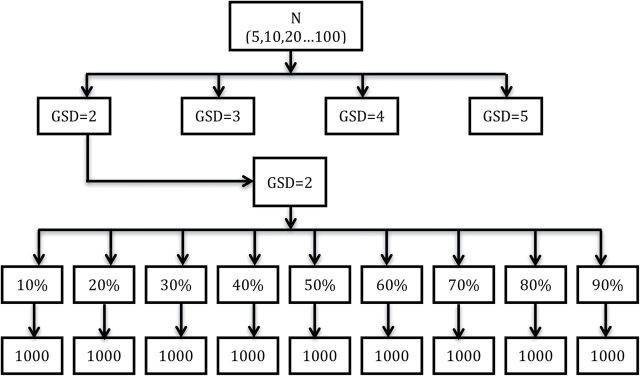
Our first simulation set represents the most basic case (Fig. 1). We generated simulated data from lognormal distributions with a true GM = 1, and true GSDs = 2, 3, 4, or 5, and a single LOD corresponding to an expected percent censoring, p, ranging from 10 to 90% in increments of 10% with varying sample sizes (5, 10, and increments of 10–100). For each of our conditions (i.e. each combination of N, GSD, and percent censoring), we generated and analyzed 1000 datasets.

Figure 1.

A graphical depiction of the simulation design. Sample sizes (N) were fixed at 5, 10, 20, 30, 40, 50, 60, 70, 90, and 100. For each sample size, simulated data were drawn from a lognormal distribution with a true GM = 1 and true GSDs of 2, 3, 4, and 5, respectively. Datasets were censored in increments of 10% with either a single LOD value or multiple LODs. For each combination of N, GM, GSD, and percent censored, 1000 datasets were generated and analyzed using the β-substitution and the Bayesian methods. A mixed lognormal distribution is created by combining two lognormal distributions with GM1 = 1 and GM2 = 5 with equal weights.

The second simulation set follows directly from the first set except we investigated the impact of multiple LODs. The issue of multiple LODs, however, is addressed differently by the two censored data methods. The β-substitution method takes the average of all the LODs and uses this average in the algorithm as if the dataset had a single LOD. This is in contrast to the Bayesian approach described in equation (2), which allows each censored observation to have a unique LOD. We simulated two scenarios (with small and large differences between the LODs) to assess the effect of the difference between the LODs. The small gap multiple LODs simulation used p ₁ = expected censoring level, p ₂ = 0.95 × p ₁, and p ₃ = 0.90 × p ₁. The large gap multiple LODs simulation used p ₁ = expected censoring level, p ₂ = 2/3 × p ₁, and p ₃ = 1/3 × p ₁. While the latter is less frequently encountered in typical occupational hygiene practice, it is more applicable to the GuLF STUDY where many EGs have highly varying values of LODs due to differences in sampling duration (4–18h).

Lastly, our third simulation attempted to model data drawn from a ‘mixed’ distribution, which in our case, is a bimodal lognormal distribution, which can occur when a limited sampling strategy or limited sampling documentation or both results in grouping disparate measurements. We simulated two types of mixed distributions (with a mixing proportion of 50/50) where one mixed distribution is a combination of two lognormal distributions with GMs of 1 and 5, and the other with GMs of 1 and 10 (see Huynh et al., 2014 for more details).

As in all simulations, the observed censoring for a given dataset may deviate from the expected censoring. Any dataset that was observed to be 100% censored was discarded because both methods used here are inappropriate for such datasets. Fully censored datasets occurred more frequently under high censoring and small sample size conditions. For a given expected censoring probability, p, and a given sample size, N, we expect to observe datasets that are fully censored with a probability $p^N$ (e.g. when N = 5 and p = 80%, the expected percent of 100% censored datasets = 32.76%).

All computation was programmed in statistical computing software R (R Development Core Team, 2014).

Priors for the simulation

In occupational hygiene practice, eliciting priors for μ and σ is often simplified by specifying a distribution and the bounds on the GM and the GSD, respectively. As such, for our comparisons we created a relatively non-informative (or ‘weakly informative’) prior for μ, which was uniformly distributed between log(0.05) and log(500). Similarly, we created a non-informative prior for σ using a uniform distribution bounded between log(1.01) and log(12) for the GSD. First, the uniform distribution was chosen over a normal distribution because the uniform distribution is generally easier to specify than a normal distribution in occupational hygiene practice. Second, the GM and GSD values were chosen such that the range was too broad to provide much information to model the simulation where the true GM = 1. We consider the priors used here to be ‘non-informative’ because their bounds are sufficiently large relative to the ‘true’ parameter values and uninformative for most occupational hygiene settings. In theory, however, one may need to use larger bounds—or perhaps unbounded distributions with a very large variance—to achieve truly non-informative priors. In order to assess the effect of narrower bounds on our posterior distributions, we also analyzed the data from our first simulation scenario using the more informative priors listed in Table 1. For the informative priors we retained the lower bound for μ, but narrowed the upper bound to In(50). We used In(1.01) and In(4) as the lower and upper bounds of σ if the true GSD =2 and 3 and In(3) and In(6) if the true GSD = 4 and 5.

Table 1.

Priors specification for μ and σ of the log-transformed data

Truth	Non-informative priors	Informative priors
μ = 0 (GM = 1)	μ ~ Uniform (ln(0.05), ln(500))	μ ~ Uniform (ln(0.05), ln(50))
σ = 0.7, 1.1, 1.4, 1.6 (GSD = 2, 3, 4, 5)	σ ~ Uniform (ln(1.01), ln(12))	σ ~ Uniform (ln(1.01), ln(4)) if true GSD = 2, 3 σ ~Uniform (ln(3), ln(6)) if true GSD = 4, 5

Evaluation metrics

Both methods were evaluated using relative bias, relative root mean squared error (rMSE), and coverage probability. Relative bias (called bias hereafter) is the difference between the average estimated value and the true value relative to the true value

$$\mathrm{Re}lativebias=100\times \frac{\bar{x}-\theta }{\theta }$$ (3)

where $\bar{x}$ is the average estimate of the parameter of interest (e.g. AM, GM, GSD, or X_0.95) from the 1000 trials, and θ is the true value. Bias can be negative or positive; negative bias indicates underestimation of the true value of the parameter while positive bias indicates overestimation. The relative rMSE is a measure that combines the bias and the precision of the method relative to the true value and can only be positive. The rMSE is generally considered a better metric than bias because rMSE allows the additional evaluation of the precision of the method.

$$RelativerMSE=100\times \frac{1}{\theta }\sqrt{{\left(\bar{x}-\theta \right)}^2+\frac{{{\displaystyle \sum }}^{\text{}}{\left(x_i-\bar{x}\right)}^2}{N-1}}$$ (4)

Coverage probability is estimated as the proportion of the estimated parameters that are located within the 95% CI/credible interval. The desired coverage probability for a 95% uncertainty interval is 0.95.

A method for computing the CI for the mean of the β-substitution method was not provided in the original paper, so we adapted an algorithm that was intended for non-censored data (by reducing the degrees of freedom to equal the number of detectable measurements) (Hewett and Ganser, 1997; P. Hewett, personal communication) to compute the CI for the AM from β-substitution method. This approach allows us to compare the coverage for the AM for the β-substitution and the Bayesian methods. We found no method to estimate the β-substitution CIs for the GM, GSD, or X_0.95, and thus, make no coverage comparisons for these parameters.

RESULTS

The results for the lognormal distributions with a single LOD and with small gap multiple LODs simulations were generally very similar. Therefore, only figures for the single LOD simulation set for the AM, GSD, and X_0.95 are shown in herein. Figures for the GM, for simulations with larger gaps between the multiple LODs and simulations with mixed distributions are shown in the Supplementary Data online. The estimated bias and rMSE for all simulations are also included in the Supplementary Data online (Excel Table). In these figures, the mean relative bias and rMSE of the 1000 datasets for each of the four parameters (GM, GSD, AM, X_0.95) are shown for the simulated conditions. The size of the circle in the figures corresponds to the magnitude of the mean bias or the mean rMSE on a continuous scale. The size of each circle generally falls between two of the circles identified with specific values in the legend. For the sake of brevity, we refer to GSD ≤ 3 as low variability and GSD ≥ 4 as high variability. Sample sizes of 5 are considered small, while those between 10 and 20 are considered moderate and above 20 large. Generally the smaller the bias and rMSE, the better the performance.

Lognormal distributions and single LOD

Arithmetic mean

Figure 2 shows that the Bayesian method with non-informative priors had a slightly higher bias than the β-substitution method in the estimation of the AM. The rMSE for both methods was small and comparable under most conditions (Fig. 3). The exception was under the condition of small to moderate sample sizes and high variability, where the Bayesian method had a larger bias but a smaller rMSE. The use of informative priors generally improved the accuracy and precision of the Bayesian estimates as expected.

Figure 2.

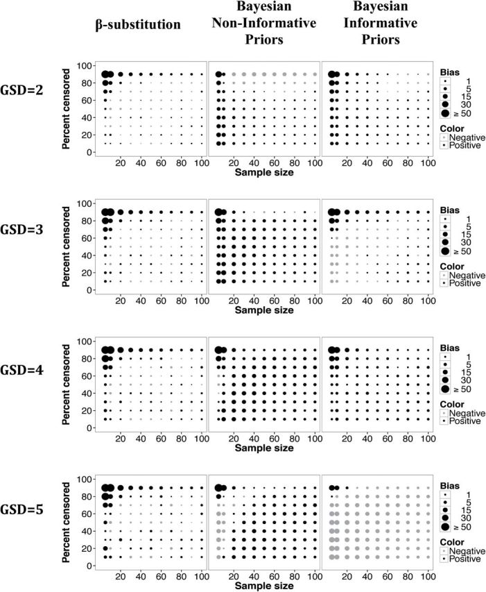
Relative bias in the estimate of the AM of a lognormal distribution and a single LOD for different sample sizes, percent censoring, and GSDs for the β-substitution method and the Bayesian method with non-informative and informative priors.

Figure 3.

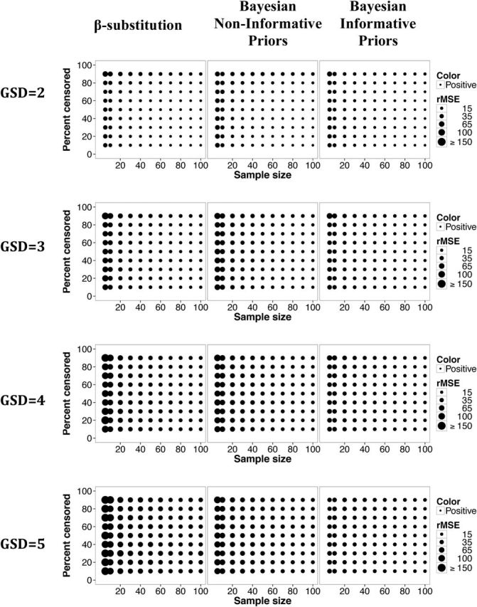
Relative rMSE in the estimate of the AM of a lognormal distribution and a single LOD for different sample sizes, percent censoring, and GSDs for the β-substitution method and the Bayesian method with non-informative and informative priors.

Figure 4 illustrates the estimated coverage probabilities for the β-substitution and the Bayesian methods for the AM. The Bayesian models with non-informative and informative priors generally provided coverage comparable to the β-substitution method in many simulated conditions. The exceptions were the condition of small sample sizes and censoring >40% and also the combination of large Ns and low censoring conditions where the β-substitution method performed worse. The results show that the β-substitution method did not provide as good of coverage as the Bayesian method.

Figure 4.

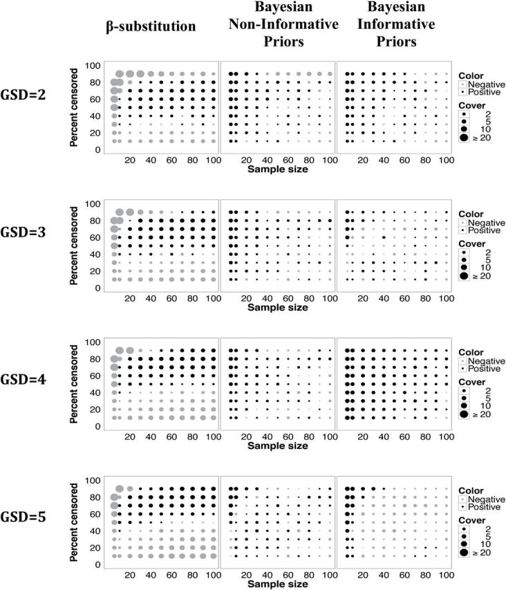
Coverage probabilities (in percent) for the AM of a lognormal distribution and a single LOD for the β-substitution method and the Bayesian method with non-informative and informative priors. The size of the circle represents difference between the actual coverage probability minus the target 95%. Positive dots indicate probabilities larger than 95%. The difference can only be up to 5% in the positive direction (indicating 100% coverage), whereas negative dots indicate probabilities less than 95%. While 100% coverage is not as desirable because the uncertainty estimates maybe too wide to be informative, large negative coverage (approximately <90%) might be worse because it indicates that the interval frequently missed the true value.

Geometric mean

The bias for the GM for the Bayesian method with non-informative priors and the β-substitution method were comparable for large sample sizes and when censoring ≤80% conditions (Supplementary Figs 1 and 2 online). The β-substitution method tended to overestimate the GM under all conditions, whereas the Bayesian method with non-informative priors tended to underestimate the GM, and with informative priors generally had mixed overestimation and underestimation.

Despite the differences in bias, the rMSE for the GM for both methods appeared to be similar. This discrepancy is likely due to the contribution of the ‘precision’ component of rMSE—i.e. the Bayesian approach provides equally (or perhaps more) precise results than the β-substitution method, thus offsetting the differences in bias. As for coverage, the β-substitution method does not currently provide an estimate for the uncertainty in GM, but the 95% CI from the Bayesian approach consistently provided coverage near the ideal probability of 0.95 (data not shown).

Geometric standard deviation (GSD)

The β-substitution method generally had smaller bias than the Bayesian method with non-informative priors but with informative priors the Bayesian method was more comparable to the β-substitution method (Fig. 5). Under conditions of small to moderate sample sizes and high censoring conditions, as the GSD increased, the bias for the β-substitution method increased, while the bias of the Bayesian method with non-informative priors decreased. This latter trend was likely influenced by the selection of the non-informative priors. As the true GSD moved closer to the median of the GSD of the prior distribution (i.e. GSD prior = (1.1 + 12)/2 = 6.5), the Bayesian model was able to provide a better estimate of the GSD (i.e. with lower bias). Thus, if a uniform ‘non-informative’ prior for the GSD is used, the Bayesian method will perform better if the median of the uniform distribution approaches the truth.

Figure 5.

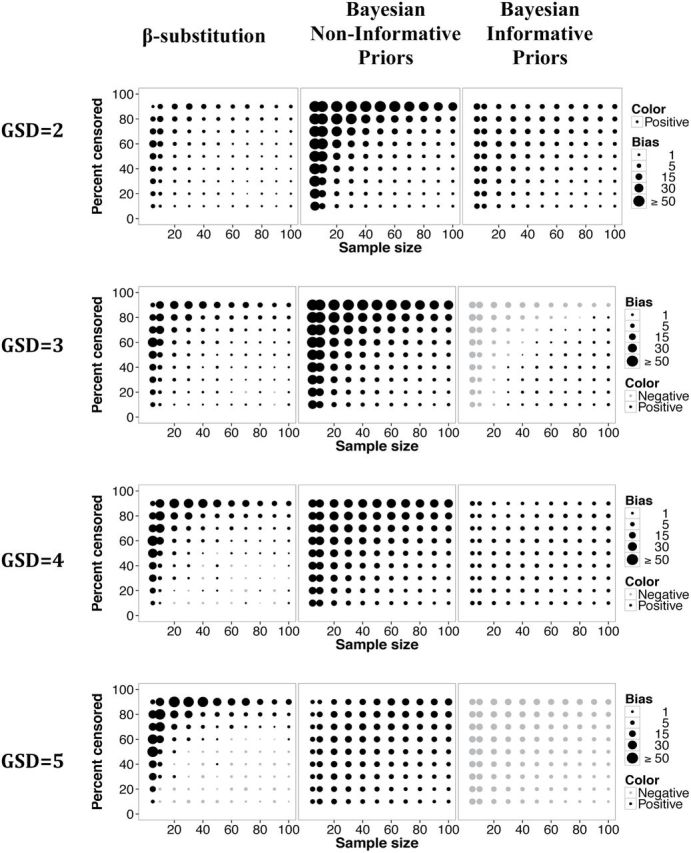
Relative bias in the estimate of the GSD of a lognormal distribution and a single LOD for different sample sizes, percent censoring, and GSDs for the β-substitution method and the Bayesian method with non-informative and informative priors.

The Bayesian method generally had a smaller rMSE than the β-substitution method, indicating better precision (Fig. 6), particularly when informative priors were used. The β-substitution method tended to provide large GSDs more frequently than the Bayesian method with non-informative priors whereas the bounded informative priors for the GSD limited the Bayesian method’s ability to provide larger GSDs (data not shown).

Figure 6.

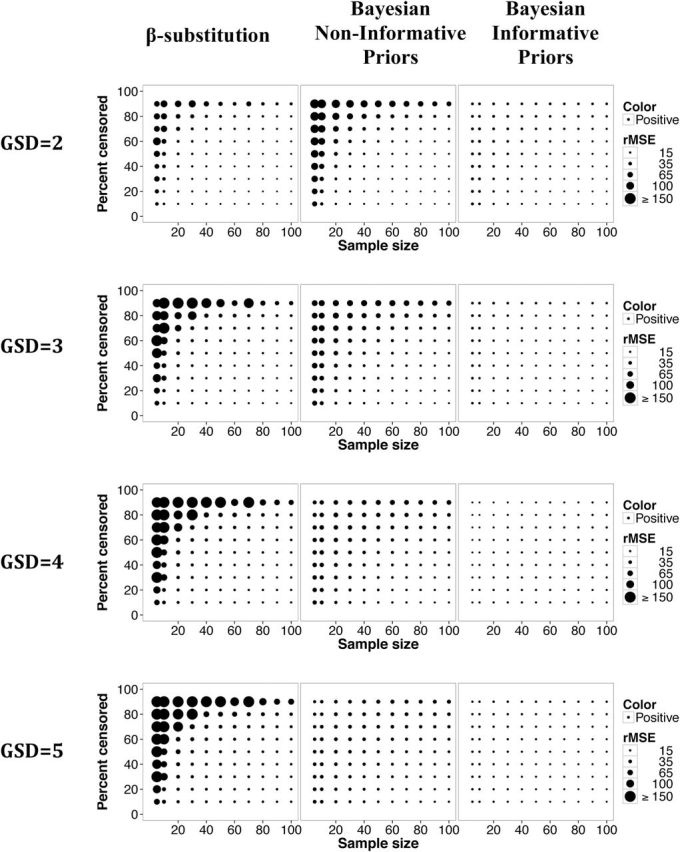
Relative rMSE in the estimate of the GSD of a lognormal distribution and a single LOD for different sample sizes, percent censoring, and GSDs for the β-substitution method and the Bayesian method with non-informative and informative priors.

While the β-substitution method failed to provide measures of uncertainty for estimates of the GSD, the 95% credible intervals generated by the Bayesian method provided the desired coverage probability of 0.95 (data not shown).

95th percentile (X_0.95)

The β-substitution method generally provided smaller bias than the Bayesian method in the estimation of the X_0.95, although the use of informative priors reduced the bias for the Bayesian method (Fig. 7). With respect to the rMSE metric, the β-substitution method and the Bayesian method generally provided comparable rMSEs for sample sizes ≥20 (Fig. 8). For smaller sample size conditions, the β-substitution method generally had a smaller rMSE than the Bayesian method with non-informative priors and comparable rMSE to the method with informative priors. As with the other parameters the coverage probability for the Bayesian method was generally close to the target coverage of 0.95 (data not shown).

Figure 7.

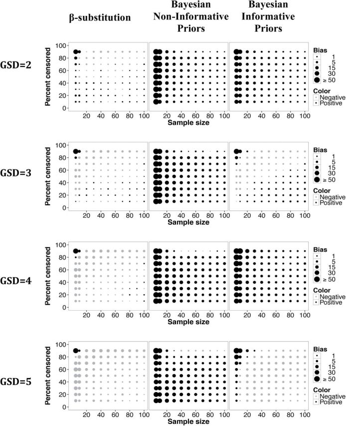
Relative bias in the estimate of the 95th percentile of a lognormal distribution and a single LOD for different sample sizes, percent censoring, and GSDs for the β-substitution method and the Bayesian method with non-informative and informative priors.

Figure 8.

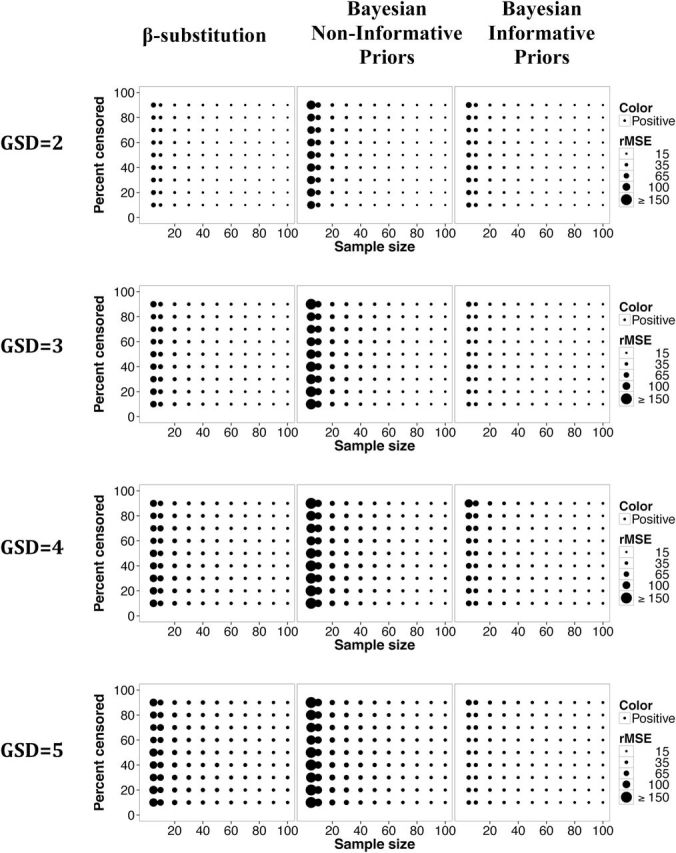
Relative rMSE in the estimate of the 95th percentile of a lognormal distribution and a single LOD for different sample sizes, percent censoring, and GSDs for the β-substitution method and the Bayesian method with non-informative and informative priors.

Other simulations

In the multiple LODs simulation where the gaps between LODs were large, the bias and rMSE in the estimation of the AM and the GM for both methods were generally comparable under most conditions (Supplementary Figs 3 and 4 for the AM and Supplementary Figs 5 and 6 for the GM are available at Annals of Occupational Hygiene online ). The β-substitution method generally had higher bias in the estimation of the AM than the Bayesian method at censoring >60% and a higher rMSE for small to moderate sample sizes and high variability. The coverage of the mean for the β-substitution method was generally much lower than the target probability of 0.95 compared to the Bayesian method’s coverage, especially at ≥60% censoring and higher variability, even with large sample size conditions (Supplementary Fig. 7 online). In the estimation of the GSD, the β-substitution method and the Bayesian method provided comparable bias and rMSE for large sample sizes except at censoring >80% (bias) and small to moderate sample sizes (rMSE) (Supplementary Figs 8 and 9 online). Lastly, in the estimation of the 95th percentile, the β-substitution method generally provided comparable or smaller bias (particularly when the variability was low) and rMSE than the Bayesian method, particularly under small sample sizes conditions (Supplementary Figs 10 and 11 online). The general poor performance of β-substitution method under some conditions might be because the β-substitution uses an averaged LOD that substantially deviated from the original LODs, whereas the Bayesian method used each of the original LODs. This type of scenario occasionally occurs in classic exposure assessment where sample duration deviates from the common practice of monitoring full-shift exposures. Variability in the LODs may occur more often, however, in (1) in task-based monitoring or (2) retrospective occupational exposure assessments that use data from multiple sources, some of which were collected many years ago or that did not incorporate full-shift monitoring. The Bayesian coverage for the GM, GSD, and X_0.95 were generally close to the target probability.

Figure 9.

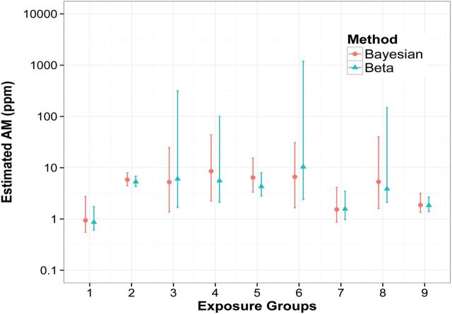
Preliminary estimates of the AM and their uncertainty using the β-substitution method and the Bayesian method with non-informative priors for nine exposure groups using GuLF STUDY data.

The results for the simulation of mixed distributions with the GMs of 1 and 5 looked very similar to those of lognormal distributions with a single LOD (figures not shown). This was likely due to the fact that the overall distribution looked more lognormal than bimodal. As the distance between the modes increased (i.e. GM₁ = 1 and GM₂ = 10), the bias for the estimation of the AM derived from the Bayesian method with non-informative priors was higher than the β-substitution method but the rMSE for both methods was small and comparable (Supplementary Figs 12 and 13 online). The β-substitution method also appeared to perform better than the Bayesian method in the estimation of the X_0.95 as shown in Supplementary Figs 14 and 15 online. In terms of coverage, the Bayesian method had much lower coverage at GSD = 2 compared to the other GSDs (shown in Supplementary Fig. 16 online). This observation is likely due to the fact that when the variability of the data is low and the distance between the two modes is large, the two modes were more distinct (the variance for each peak is small), causing the uncertainty intervals computed from the simulated data to miss the true value more often compared to when the variability of the data is higher. For GSD = 2, the coverage for the β-substitution method and the Bayesian method were equally poor but at higher GSD, the Bayesian coverage was slightly better than for the β-substitution method as in the single LOD and multiple LOD simulations.

An illustrated example

To further demonstrate the behavior of the β-substitution and the Bayesian methods, we analyzed a small subset of the GuLF STUDY data using both methods. The THC exposure assessment component of the study involves analysis of about 25 000 personal measurements, which is the motivation for the simulation study.

We used somewhat non-informative (weakly informative) priors for the Bayesian method as follows:

$$\begin{array}{l}\mu ~\text{ Uniform }(\text{ln}\left(0.0\text{5}\right),\text{ln}\left(\text{5}0\right))\\ \sigma ~\text{ Uniform }(\text{ln}\left(\text{1}.0\text{1}\right),\text{ln}\left(\text{12}\right))\end{array}$$

The notation for μ denotes a uniform distribution with a minimum GM of 0.05 and a maximum of 50. The lowest LOD in the THC measurements was 0.064 p.p.m. and only 0.57% was below 0.10 p.p.m. Based on BP documents, various actions, including use of respirator protection, were triggered to reduce exposures to THC when direct reading volatile organic compound measurements exceeded 100 p.p.m. for greater than 15min (BP, 2010). In this particular example, we used a GM maximum of 50 p.p.m. to already account for the large amount of uncertainty. The prior for σ takes a uniform distribution with the minimum and maximum GSDs of 1.01 and 12, respectively. We used JAGS to run the Bayesian model (Plummer, 2003) and R to process results.

Figure 9 and Supplementary Table 2 online show the results of our analysis for nine preliminary EGs for THC measured on one of the rig vessels during the Deepwater Horizon response. The AM estimates for both methods were comparable for most EGs. The upper bounds of the 95% CI for the β-substitution method, however, were higher than those of the Bayesian method for a few groups. In contrast, because the GSD estimates from the Bayesian method had been restricted by the maximum prior (i.e. GSD = 12), some of the Bayesian GSDs were close to the upper bound, but did not exceed it because of the boundary requirements. A sensitivity assessment of the priors (i.e. reanalyzing the data using an unbounded uniform prior or a prior with a larger upper bound) would likely result in the Bayesian method providing higher estimates of the GSD.

DISCUSSION

The β-substitution method and the Bayesian method with non-informative priors often produced accurate point estimates for many of the simulated conditions. Both methods’ performance varied, however, when estimating differing parameters. Generally, the Bayesian method with non-informative priors was comparable to the β-substitution method when estimating the AM and GM but it was more biased in the estimation of the GSD and the 95th percentile, although the use of more informative priors resulted in more comparable performances. The Bayesian method generally provided consistent and better coverage of the AM than the β-substitution method.

The β-substitution method’s ease of implementation in a simple spreadsheet can be an attractive feature to many practitioners. If, however, coverage (i.e. an uncertainty interval) is important, which was one motivation for this work, this method is not recommended. It currently does not have a method for providing uncertainty estimates for the GM, GSD, or X_0.95. Even for the AM, we had to adapt a method for non-censored data described by Hewett and Ganser (1997) to allow comparison with the Bayesian 95% CI. It is possible that this adaptation was not appropriate for censored data and that this was the reason that the 95% CI of the β-substitution method was not able to provide the coverage comparable to the Bayesian method or close to the ideal coverage probability of 0.95. Although methods for deriving uncertainty intervals for β-substitution have not yet been described elsewhere, other approaches to compute the CI might be feasible (Helsel, 2005) and could result in coverage comparable to the Bayesian approach described here. However, it is beyond the focus of this paper to test various ways to compute the CI for the β-substitution method.

Under the condition of multiple LODs that were much further apart, the β-substitution method performed worse than the Bayesian method because β-substitution method uses an averaged LOD that, in many cases, substantially deviated from the original LODs, whereas the Bayesian method used each of the original LODs. This type of scenario (i.e. multiple LODs) is infrequently encountered in typical exposure assessments but may occur in retrospective occupational exposure assessments that often use multiple sources of data for the estimation of historical exposure levels. The second reason for the simulation study was to obtain accurate point estimates for the AM, GM, GSD, and X_0.95 of the lognormal data. While this is the scenario that the β-substitution method was designed for, it is not clear if this approach can be used for inference in other types of statistical analyses such as regression and analysis of variance that can be used to form appropriate EGs. In contrast, however, Bayesian methods like those used here can incorporate censoring for these types of models as well as correlated data problems like those seen in spatial analyses.

The performance of the Bayesian method depends on the choice of priors, which will vary with different studies. As stated earlier, the non-informative priors chosen for the simulation are occupational hygiene specific and the range of the minimum and maximum values are not appropriate for other types of studies (for example, data that could have GMs much lower than our simulated GMs). As for informative priors, different informative priors might have different influences on the posterior distribution that cannot be captured in a simulation study. Thus, any detailed insights (such as the direction or magnitude of bias) from these informative prior simulations, other than that they improved the Bayesian method’s performance over the non-informative priors, might not be appropriate. While the Bayesian method generally can provide accurate point estimates and a full distribution for all the parameters using relatively non-informative priors, good priors may be difficult to identify under conditions where they are needed most, i.e. small sample sizes or high censoring. In addition, some computational skills are also needed to obtain the full benefits of the Bayesian methods. The JAGS and R codes for the Bayesian censored data are provided in the Supplementary Data online to assist readers.

Our simulation study attempted to assess a wide range of conditions; however, as with any simulation study, these conditions might not be representative of all the conditions that one might encounter in an occupational exposure assessment study. We tested the mixed distribution simulation to assess how far we can stretch the lognormality assumption for these parametric methods and found that the Bayesian method (using non-informative priors) generally did not work well for censored data that were substantially bimodal. Since most exposure data generally have a lognormal distributional shape, this assumption might not be important, and if the modes are close enough, the Bayesian method might suffice. However, if the data are distinctively bimodal, the results from the Bayesian method might be less predictable than the β-substitution method.

CONCLUSION

Our simulation study compared the β-substitution method and a Bayesian method for estimating parameters of exposure distributions with censored data. We have shown that both methods generally delivered accurate point estimates, while only the Bayesian method provided reliable uncertainty intervals for all four parameters investigated. The β-substitution method was generally less biased and was easier to implement but its measure of uncertainty was less reliable for the AM, and uncertainty could not be estimated for the other parameters. We recommend that the practitioner take into account the data available, the purpose of the estimation, and the need for uncertainty estimates when selecting a method with censored data. Bayesian methods may be particularly useful if the practitioner has the computational resources necessary and prior information, as the methods would generally provide accurate point estimates and also the distributions of all of the parameters.

SUPPLEMENTARY DATA

Supplementary data can be found at http://annhyg.oxfordjournals.org/.

FUNDING

This work is funded in part by the Intramural Research Program of the NIH, National Institute of Environmental Health Sciences, ZO1 ES 102945.

DECLARATION

The contents of this paper, including any opinions and/or conclusions expressed, are those of the authors alone and do not necessarily reflect the policy of the NIEHS.

REFERENCES

- Aitchison J, Brown JAC. (1957) The lognormal distribution with special reference to its uses in economics. Cambridge, UK: Cambridge University Press. [Google Scholar]
- Antweiler RC, Taylor HE. (2008) Evaluation of statistical treatments of left-censored environmental data using coincident uncensored data sets: I. Summary statistics. Environ Sci Technol; 42: 3732–8. [DOI] [PubMed] [Google Scholar]
- BP. (2010) Gulf of Mexico Drilling, Completions and Interventions. Deepwater Horizon MC252 Response Offshore Air Monitoring Plan for Source Control. Internal BP document.
- Busschaert P, Geeraerd AH, Uyttendaele M, et al. (2011) Hierarchical Bayesian analysis of censored microbiological contamination data for use in risk assessment and mitigation. Food Microbiol; 28: 712–9. [DOI] [PubMed] [Google Scholar]
- Carlin BP, Louis TA. (2009) Bayesian methods for data analysis. 3rd edn. Boca Raton, FL: Chapman and Hall/CRC Press. [Google Scholar]
- Cohen AC. (1959) Simplified estimators for the normal distribution when samples are singly censored or truncated. Technometrics; 1: 217–37. [Google Scholar]
- Cohen AC. (1961) Tables for maximum likelihood estimates: singly truncated and singly censored samples. Technometrics; 3: 535–41. [Google Scholar]
- Finkelstein MM, Verma DK. (2001) Exposure estimation in the presence of nondetectable values: another look. Am Ind Hyg Assoc J; 62: 195–8. [DOI] [PubMed] [Google Scholar]
- Finney DJ. (1941) On the distribution of a variate whose logarithm is normally distributed. J R Stat Soc; 7 (Suppl): 155–61. [Google Scholar]
- Fisher RA. (1925) Theory of statistical estimation. Proc Camb Philos Soc; 22: 700–25. [Google Scholar]
- Flynn MR. (2010) Analysis of censored exposure data by constrained maximization of the Shapiro – Wilk W statistic; 54 263–71. 10.1093/annhyg/mep083 [DOI] [PubMed] [Google Scholar]
- Ganser GH, Hewett P. (2010) An accurate substitution method for analyzing censored data, J Occup Environ Hyg; 7: 233–44. [DOI] [PubMed] [Google Scholar]
- Gelfand AE, Smith AFM, Lee TM. (1992) Bayesian analysis of constrained parameter and truncated data problems using Gibbs sampling. J Am Stat Assoc; 87: 523–32. [Google Scholar]
- Gillespie BW, Chen Q, Reichert H, et al. (2010) Estimating population distributions when some data are below a limit of detection by using a reverse Kaplan-Meier estimator. Epidemiology; 21 (Suppl. 4): S64–70. [DOI] [PubMed] [Google Scholar]
- Gilliom RJ, Helsel DR. (1986) Estimation of distributional parameters for censored trace-level water-quality data. I. Estimation techniques. Water Resour Res; 22: 135–46. Available at http://pubs.er.usgs.gov/usgspubs/ofr/ofr84729. Accessed 5 July 2015 [Google Scholar]
- Helsel DR. (2005) Nondetects and data analysis. New York, NY: John Wiley & Sons, Inc. [Google Scholar]
- Helsel D. (2010) Much ado about next to nothing: incorporating nondetects in science. Ann Occup Hyg; 54: 257–62. [DOI] [PubMed] [Google Scholar]
- Helsel DR, Cohen TA. (1988) Estimation of descriptive statistics for multiple censored water quality data. Water Resour Res; 24: 1997–2004. [Google Scholar]
- Hewett P, Ganser GH. (1997) Simple procedures for calculating confidence intervals around the sample mean and exceedance fraction derived from lognormally distributed data. Appl Occup Environ Hyg; 12: 132–42. [Google Scholar]
- Hewett P, Ganser GH. (2007) A comparison of several methods for analyzing censored data. Ann Occup Hyg; 51: 611–32. [DOI] [PubMed] [Google Scholar]
- Hewett P, Logan P, Mulhausen J, et al. (2006) Rating exposure control using Bayesian decision analysis. J Occup Environ Hyg; 3: 568–81. [DOI] [PubMed] [Google Scholar]
- Hornung RW, Reed LD. (1990) Estimation of average concentration in the presence of non-detectable values. Appl Occup Environ Hyg; 5: 46–51. [Google Scholar]
- Huynh T, Ramachandran G, Banerjee S, et al. (2014) Comparison of methods for analyzing left-censored data to estimate worker’s exposures for the GuLF STUDY. Ann Occup Hyg; 58: 1126–42. [DOI] [PMC free article] [PubMed] [Google Scholar]
- Kaplan EL, Meier P. (1958) Nonparametric estimation from incomplete observations. J Am Stat Assoc; 53: 457–81. [Google Scholar]
- Krishnamoorthy K, Mallick A, Mathew T. (2009) Model based imputation approach for data analysis in the presence of non-detectable values: normal and related distributions. Ann Occup Hyg; 59: 249–68. [DOI] [PubMed] [Google Scholar]
- Kroll CN, Stedinger JR. (1996) Estimation of moments and quan-tiles using censored data. Water Resour Res; 32: 1005–12. [Google Scholar]
- Leidel NA, Busch KA, Lynch JR. (1977) Occupational exposure sampling strategy manual. National Institute for Occupational Safety and Health Pub. No. 77–173 (available from the National Technical Information Service, Pub. No. PB274792) Available at http://www.cdc.gov/niosh/docs/77-173/pdfs/77-173.pdf. Accessed 5 July 2015. [Google Scholar]
- Mulhausen J, Damiano J. (2006) Chapter 4, Establishing similar exposure groups. In Ignacio JS, Bullock WH, editors. A strategy for managing occupational exposures. 3rd edn. Fairfax, VA: AIHA Press; pp. 33–46. [Google Scholar]
- Paulo MJ, Van der Voet H, Jansen MJW, et al. (2005) Risk assessment of dietary exposure to pesticides using a Bayesian method. Pest Manage Sci; 61: 759–66. [DOI] [PubMed] [Google Scholar]
- Plummer M. (2003) JAGS: a program for analysis of Bayesian graphical models using Gibbs sampling. Proceedings of the 3rd International Workshop on Distributed Statistical Computing (DSC 2003), March 20–22, Vienna, Austria. ISSN 1609-395X. Available at http://mcmc-jags.sourceforge.net/ Accessed 23 September 2014.
- R Development Core Team. (2014) R: a language and environment for statistical computing. Vienna, Austria: R Foundation for Statistical Computing; Available at http://www.R-project.org Accessed 23 September 2014. [Google Scholar]
- Rappaport SM. (1991) Assessment of long-term exposures to toxic substances in air. Ann Occup Hyg; 35: 61–122. [DOI] [PubMed] [Google Scholar]
- Singh A, Maichle R, Lee SE. (2006) On the computation of a 95% upper confidence limit of the unknown population mean based upon data sets with below detection limit observations. Washington, DC: U.S. Environmental Protection Agency. EPA/600/R-06/022. [Google Scholar]
Associated Data
This section collects any data citations, data availability statements, or supplementary materials included in this article.