The functional diversity of retinal ganglion cells in the mouse

SUMMARY

In the vertebrate visual system, all output of the retina is carried by retinal ganglion cells. Each type encodes distinct visual features in parallel for transmission to the brain. How many such “output channels” exist and what each encodes is an area of intense debate. In mouse, anatomical estimates range between 15–20 channels, and only a handful are functionally understood. Combining two-photon calcium imaging to obtain dense retinal recordings and unsupervised clustering of the resulting sample of >11,000 cells, we here show that the mouse retina harbours substantially more than 30 functional output channels. These include all known and several new ganglion cell types, as verified by genetic and anatomical criteria. Therefore, information channels from the mouse’s eye to the mouse’s brain are considerably more diverse than shown thus far by anatomical studies, suggesting an encoding strategy resembling that used in state-of-the-art artificial vision systems.

Visual processing begins in the retina (reviewed in¹). Here, photoreceptors feed into bipolar cells², which provide input to a diverse set of retinal ganglion cells (RGCs). Each type of RGC tiles the retinal surface and extracts specific features of the visual scene for transmission to the brain. However, it is still unclear how many such parallel retinal “feature channels” exist, and what they encode.

Early studies classified cells into ON, OFF or ON-OFF and transient or sustained types (e.g.^3,4) based on the response of individual RGCs to light stimulation. These studies also identified RGC types selective for local motion, motion direction or uniform illumination^3,5–7. In the most complete physiological survey to date, Farrow and Masland⁸ clustered ~450 mouse RGCs by their light responses into 12+ functional types using multi electrode array (MEA) recordings, suggesting a similar number of feature channels in the retina. In contrast, anatomical classifications of RGC dendritic morphologies estimated around 15–20 types (e.g.^9–12). Recently, Sümbül and co-workers¹⁰ found 16+ types using unsupervised clustering together with genetic markers. If each of these anatomically distinct types performed one function, there should be no more than ~20 retinal output channels.

Commonly, RGCs of the same “genuine” type are thought to share the same physiology, morphology, intra-retinal connectivity, retinal mosaic, immunohistochemical profile and genetic markers. Whether these features suffice to define a type and how classification schemes should be organised is the matter of a long-standing debate^13–16. For example, if also axonal projections were considered type-specific, this could result in a much greater variety of retinal output channels. In zebrafish, RGCs show at least 50 unique combinations of “dendro-axonal RGC morphologies” targeting a total of 10 anatomically defined projection fields¹⁷. RGCs in mice project to 40+ targets¹⁸, suggesting that there may be an even larger number of mouse RGC types.

Reliably recording from all RGC types

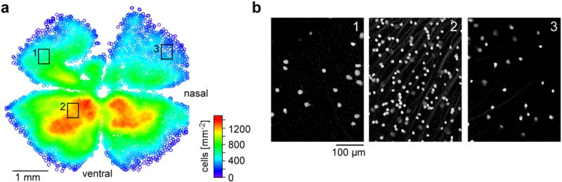
Here, we sought to test this idea and determine the number of functional output channels of the mouse retina, to obtain a complete picture of what the mouse’s eye tells the mouse’s brain. We used two-photon Ca²⁺ imaging to record light-evoked activity in all cells within a patch of the ganglion cell layer (GCL). Cells were loaded with the fluorescent Ca²⁺ indicator Oregon-Green BAPTA-1 (OGB-1) by bulk electroporation¹⁹ (Fig. 1a_1,2). This approach resulted in near-complete (>92%) staining of GCL cells, with less than 1% damaged cells²⁰. To acquire a patch of several hundreds of cells, we recorded up to 9 neighbouring 110 × 110 μm fields (at 7.8 Hz), each containing 80 ± 20 GCL somata (Fig. 1a_1,2, cf. SI Video 1). In total, >11,000 cells were sampled.

Figure 1. Data collection.

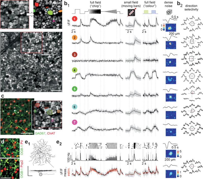
a, whole-mounted mouse retina, electroporated with OGB-1 and recorded with a two-photon microscope (64×64 pixel @ 7.8 Hz) in the GCL. Scan fields (a₁, left; 110×110 μm) comprised 80 ± 20 cells. Regions-of-interest (ROIs) (a₁, right), were placed semi-automatically. Montage (a₂) of 9 consecutively recorded fields (rectangles; a₁ in red). b, Ca²⁺ signals from 7 ROIs colour-coded in (a₁). Single trials in grey, averages of n=4 (“chirp”, green/blue) or 24 (moving bars) trials in black (b₁). Responses to 4 visual stimuli (b₁): Full-field “chirp”, bright bars moving in 8 directions, full-field alternating green/blue and binary noise for space-time kernels. Direction- and orientation-selectivity (b₂): Traces by motion direction; polar plot of peak response, vector sum in red. c, left: experiment in (a) immunostained for GAD67 (green; GABAergic ACs) and ChAT (red; starburst-ACs). Right: from (a₁); both images show same colour-coded ROIs (left, dots, right, ROI outlines) and starburst-ACs (white dots): cell 6 is GAD67-positive, cell 7 is a starburst-AC. d, OGB-1 (green) electroporated retina from transgenic mice with tdTomato (red) expressed in sets of RGCs (top: PV; bottom: Pcp2). e, simultaneous Ca²⁺ imaging and electrical recording: dye-filled, anatomically reconstructed cell (e₁, top: whole-mount; bottom: profile, lines mark ChAT bands). Light responses (e₂) from top to bottom: spike raster and rate (20 ms bins), recorded (black) and reconstructed (orange) Ca²⁺ signal. Scale bars: 50 μm unless indicated.

We presented four light-stimuli (Fig. 1b): (i) a full-field “chirp”-stimulus to characterise polarity, kinetics and the preference for temporal frequencies and contrasts, (ii) a moving bar to probe for direction and orientation selectivity (Fig. 1b₂), (iii) binary dense noise to estimate receptive fields and (iv) an alternating long- / short-wavelength (“green/blue”) full-field stimulus to probe for chromatic preference (Methods). This set of stimuli was chosen to cover a large stimulus-space that distinguishes different response types.

We performed recordings in the ventral retina, as verified by the mean chromatic response preference^21,22 of each imaged field (Extended Data Fig. E1e), to control for retinotopic sources of variability^23–25. In addition, we always presented stimuli at the same light levels in the low photopic regime (Methods).

Our approach allowed us to determine the soma size and position of each recorded cell. Immunohistochemistry (Methods) was used in a subset of experiments: displaced amacrine cells (dACs), which are GABAergic and/or cholinergic and represent a substantial fraction of GCL somata²⁶, were labelled for GAD67 and ChAT (Fig. 1c; n=522 of 1,584 cells; double-labelled: n=96). Melanopsin-labelling^27,28 identified strongly melanopsin-expressing intrinsically-photosensitive RGCs (ipRGCs, n=18 of 905 cells). SMI-32 labelled a small set of GCL cells (n=85 of 1,912 cells), including starburst dACs²⁹, and was used to identify alpha RGCs (large, strongly-labelled somata^9,23). In addition, we performed recordings in two transgenic lines, PV and Pcp2 (Methods; Fig. 1d), to relate individual recorded cells to known genetically-defined populations.

Finally, we made electrical single-cell recordings from RGCs (n=84) followed by dye-filling to reconstruct their dendritic morphology (Fig. 1e₁). For all cells with Ca²⁺ and spike activity recorded simultaneously (n=17), Ca²⁺ responses estimated from spike trains closely resembled measured Ca²⁺ responses (Fig. 1e₂; Extended Data Fig. E1a–d).

A probabilistic clustering framework

Combining locally complete optical population recordings, genetic and immunohistochemical labels, as well as electrical measurements, yielded a comprehensive dataset of GCL cell light responses to a set of standardised visual stimuli. This provided the unprecedented opportunity for an unbiased characterisation of the retinal output. Since the dataset (11,210 cells, n=50 retinas; Extended Data Fig. E2) is too complex to be interpreted manually (e.g.³⁰), we used a clustering approach, making our analysis as objective and quantitative as possible.

In the first step, we used an automatic unsupervised clustering procedure to identify response prototypes of GCL cells (Extended Data Fig. E2d,e₁; Methods). Specifically, we used sparse Principal Component Analysis (sPCA) to extract features from the light-driven Ca²⁺ signals of the GCL cells (Methods), which identified many classically used temporal response features such as ON- and OFF responses with different kinetics or selectivity to different temporal frequencies. We then used a Mixture of Gaussian model on this feature set for clustering (Methods). In the second step, we post-processed the clustered data to make it accessible for interpretation, including the identification of clusters corresponding to dAC types based on GAD67 staining and isolation of alpha RGCs⁹ with large somata from similarly responding cells (Extended Data Fig. E2e₂,f–h). The validity of this step was verified in detail below (see Example RGC types).

Finally, we arranged the clusters according to a hierarchical tree based on their functional similarity (Methods) and suggest a grouping scheme based on available domain-knowledge (Fig. 2a–c). Some groups span different branches, as the tree was solely based on the functional response features.

Figure 2. Functional RGC types of the mouse retina.

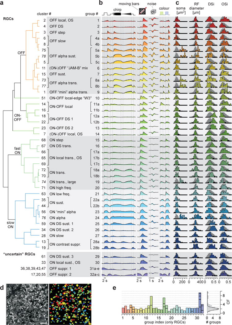
a, cluster-dendrogram (Methods) with groups indicated: n=28 RGC and n=4 “uncertain” RGC groups. b, cluster-mean Ca²⁺ responses to the 4 stimuli. c, selected metrics, from left to right: ROI (soma) area, receptive field (RF) diameter (2 s.d. of Gaussian), DS-index and OS-index (Methods). Background-histograms demarcate all RGCs. d, experiment (left, from Fig. 1a₂) with RGCs colour-coded by group (right). dACs and discarded cells not shown. e, Coverage factor (CF) calculated from RF-area for RGC groups, with horizontal divisions delineating individual clusters (left) and distribution of CFs across groups (right). Scale bar in d, 50 μm.

This framework yielded a total of 46 groups (n=7,982 cells, 71.2% of all cells, Extended Data Fig. E2f), divided into 32 RGC groups (n=5,024, 62.9% of grouped cells; including 4 groups, G_29–32, from “uncertain” clusters) and 14 dAC groups (n=2,958, 37.1% of grouped cells). The estimated fraction of dACs (between 37.1% and 50.6%, if including all “uncertain” groups) is within the expected range²⁶. We did not analyse dACs in detail (see Extended Data Fig. E3a–c; SI Video 2; SI Data 1_50–75; SI Discussion).

A minimum of 32 mouse RGC types

The identified 32 RGC groups comprised non-DS (9 OFF, 12 ON, 3 ON-OFF) and DS (2 ON-OFF, 4 ON, 2 OFF) groups (Fig. 2a–c; SI Data 2_1–32) and accounted for all known RGC types in the mouse retina¹⁵. This includes groups corresponding to three alpha types³¹ (G_5,8,24, see also below), ON-OFF³² (G_12,13) and ON DS types³³ (G_16,25,26,29), JAM-B (ref²⁴) (G₆) and W3 cell²⁵ (G₁₀), and the OFF “suppressed-by-contrast” cell³⁴ (G_31,32). The allocation of cells to individual groups was uniform across space (Fig. 2d) and the fraction of the population accounted for by broad response types was consistent across experiments (Extended Data Fig. E3e).

As each RGC type is thought to tile the retina, we calculated each group’s functional coverage factor (CF) based on its average receptive field (RF) size and its relative abundance (Extended Data Fig. E4; Methods). A single RGC type would yield a CF of 1 without RF overlap, and a CF of ~2 with 30% overlap. A CF<<1 may indicate that a type has been artificially split.

The average CF across all RGC groups was 2.0 ± 0.7 (mean ± s.d. of Gaussian fit, Fig. 2e), broadly consistent with reported CFs for mouse RGCs (roughly 2–3; see SI Table 1 and SI Discussion). CFs higher than 2 may indicate groups consisting of multiple types: For example, G₁₂ corresponding to ON-OFF DS cells³² (cf. Fig. 4a), has a CF of 7.7, consistent with 4 ON-OFF DS types, each preferring a different motion direction³⁵ (see below). The mixed non-DS groups G₁₇ and G₃₁ likely contain more than one type, supported by multiple distinct morphologies and genetic identities (e.g. G_31,32, Extended Data Fig. E5) or response properties (e.g. G₁₇, see below).

Figure 4. Direction- and orientation-selectivity.

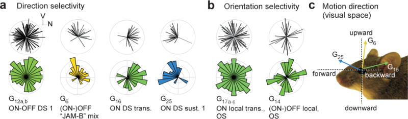
a, pairs of retinocentric polar plots showing distributions of preferred motion directions of selected direction-selective (DS) RGC groups (V, ventral; N, nasal). Top, plot of each pair: preferred directions, with length representing DSi and grey level p(DS) (Methods). Bottom, plot of each pair: circular area-normalised histogram. b, like (a), selected orientation-selective (OS) RGCs. Further DS/OS groups detailed in Extended Data Fig. E7. c, motion directions in the visual space of the mouse.

Taken together, our CF analysis suggests that the number of unique functional RGC types in the mouse is substantially above 32, likely as high as 40, in particular since classical ipRGCs (i.e. M1) as well as at least one PV-positive small-field RGC type were largely discarded based on their low S/N response to our stimuli (see SI Discussion). This is about three times the highest number of physiologically defined RGC types to date⁸ and about twice the highest anatomical diversity reported in mouse¹¹ (SI Table 2).

Example RGC types

There are three types of alpha cells known in the mouse retina³¹: the sustained (G₅) and transient OFF alpha (G₈) and the ON alpha (G₂₄). These cells are characterised by their large somata, a feature that we used during the post-processing step (Extended Data Fig. E2g–h). For the transient OFF and the ON alpha we found similarly responding cells with smaller somata, which we named transient OFF “mini” (G₉) and ON “mini” alpha cell (G₂₃), respectively (Fig. 3a–d). For the sustained OFF alpha (G₅) we did not identify an obvious “mini”-version.

Figure 3. Classical alpha RGCs and their “mini” counterparts.

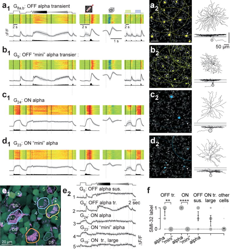
a, functional “fingerprint” of classical transient OFF alpha cells (G_8a,b). Light-evoked Ca²⁺ responses of n=80 cells (a₁): heat-maps (top) of individual responses, response averages and firing rates estimated from Ca²⁺ signals below (cf. Extended Data Fig. E1). a₂, left, G_8a,b somata (yellow) and receptive fields (RFs, dotted) indicated in example experiment (cf. Fig. 1a₂). Grey circles mark cells with RFs above quality criterion (Methods). Sample morphology of a G_8a,b cell filled after electrical single-cell recording (a₂, right). For details, see SI Data 2₈. b_1,2, G₉ RGCs (n=68), dubbed transient OFF mini alpha because of their similarity in light response to G_8a,b RGCs (cf. a_1,2). c_1,2, G₂₄ RGCs (n=44), identified as classical ON alpha. d_1,2, G₂₃ RGCs (n=113), dubbed ON mini alpha (cf. c_1,2). Mini alphas have smaller RF diameters than classical alphas (median in μm, 95% confidence interval): G₉,280 (270–293) versus G₈, 306 (294–315) with p=0.01232), and G₂₃, 236 (218–256) versus G₂₄, 319 (290–352) with p=0.00026 (rank-sum test). e, overlay of OGB-1-stained cells (green) and SMI-32 (magenta). SMI-32-positive RGCs include classical alphas (e₁, solid contours; n.r. indicates a non-responsive cell), one large-soma non-alpha cell (green, dotted contour) as well as weakly-labeled ON-OFF DS cells (dashed contours) and starburst-ACs (asterisks). Mini alpha cells (blue, dotted contours) are SMI-32-negative. Chirp-evoked Ca²⁺ responses (e₂) for 5 cells in (e₁). f, SMI-32 statistics (OFF tr.: alpha, n=16, mini, n=3; ON: alpha, n=6, mini, n=15; OFF sus. alpha, n=14; ON tr. large, n=7; other, n=957; means with 95% confidence intervals, **, p≤0.01; ****, p≤0.0001, logistic regression).

We tested whether these pairs consisted of distinct types using SMI-32 immunohistochemistry on a subset of cells (n=1,912, Fig. 3e,f). These immunolabels were not used during post-processing (Extended Data Fig. E2e₂). In an example field, all “classical” alpha cells were SMI-32-positive (#1–3; Fig. 3e). In contrast, two ON mini alphas (#4) had smaller somata and were SMI-32-negative, despite a response profile similar to the ON alpha. Across our entire set of stained cells, transient OFF and ON alpha cells were consistently SMI-32-positive, while their respective mini counterparts were not (Fig. 3f, p<0.01, generalised linear model, Methods). In addition, ON alphas, unlike their mini counterparts, were PV-positive (n_ONalpha=16/26 vs. n_ONalpha-mini=1/37, SI Data 2_23,24). Finally, alpha and mini alpha types formed independent mosaics (Fig. 3a₂–d₂). Transient OFF mini alpha cells (n=2) stratified similarly to transient OFF alpha cells (n=5), but with smaller dendritic arbours, consistent with their smaller RFs (Fig. 2c; SI Data 2_8,9; for statistics, see Fig. 3 (legend)). The same was the case for ON alpha and mini alpha RGCs (SI Data 2_23,24). Together, these data argue that indeed alphas and mini alphas are distinct cell types. The OFF sustained alpha was only moderately SMI-32-immunoreactive (Fig. 3f), consistent with previous reports²³. An additional, weakly SMI-32-positive RGC group with large somata (#5 in Fig. 3e) was dubbed “ON transient, large” (G₁₉).

The classical “local edge detector” (ref³⁶) or W3 cell²⁵ likely corresponds to G₁₀ (Extended Data Fig. E6a,b). This type had small somata and RFs, and responded poorly to full-field stimuli. Instead, G₁₀ cells reliably responded to moving bars with a brisk burst at the leading and trailing edge, consistent with previous reports²⁵. Intracellular filling confirmed the cell’s morphological identity (Extended Data Fig. E6a₃). A second group, G₁₁, had similar response properties with a reduced leading-edge response, potentially corresponding to a W3 variant²⁵.

Contrast-suppressed RGCs (e.g.^37,38) occur in many species and a type of OFF supressed-by-contrast (Sbc) cell has recently been described in mouse³⁴ (G₃₁). We found a new ON Sbc cell type (G₂₈), which responded slowly to a full-field increase in light level but was suppressed by temporal contrast (Extended Data Fig. E6c,d). One candidate morphology diffusively stratified across the entire IPL while another stratified exclusively in the ON layer.

Direction and orientation selectivity

Our RGC groups contained n=1,757 DS cells (35% of RGCs; Extended Data Fig. E7a–d; Methods). Most DS cells (70%) were sorted into 8 groups (G_{2,6,12,13,16,25,26,29}). This high functional diversity among DS cells is in agreement with studies of DS RGC-specific transgenic mouse lines³⁹. Further DS clusters were grouped with functionally similar non-DS counterparts (G₄,₁₈,₂₈), as they contained less cells than the matching non-DS clusters. These may include RGCs with slightly asymmetric dendritic arbours (e.g.¹⁰) that could lead to directional bias in response to motion. Classically, these cells are not considered DS.

To identify the motion axes of DS groups, we registered the orientation of the retina in a subset of experiments (n=3,830 cells, n=12 retinas, Fig. 4; Extended Data Fig. E7e,f). Three DS groups largely preferred one direction: the ON DS transient (G₁₆), the JAM-B RGC²⁴ (G₆) and one of the sustained ON DS cells (G₂₅) preferred backward, upward and forward motion, respectively. The other DS groups responded to more than one direction. The two groups of ON-OFF DS cells (G_12,13) contain the four classical subtypes³², with room for additional ones, as suggested by genetics and central projections (e.g.⁴⁰; SI Discussion). The three classical sustained ON DS types³³ are included in G_25,26,29.

We found two OFF DS groups (G_2,6), with G₆ containing JAM-B RGCs²⁴. These cells responded weakly to ON and strongly to OFF light changes, consistent with the JAM-B’s polarity switch with stimulus size. In addition, we identified a new OFF DS cell (G₂, Extended Data Fig. E6e,f). This group did not co-stratify with the ChAT bands, which play a role in most known DS circuits (reviewed in³⁹). Morphology, response profile, and directional preference of G₂ suggests that these cells are not the JAM-B RGCs (see above).

As predicted by recordings from mouse lateral geniculate nucleus⁴¹ and superior colliculus⁴², we identified n=730 (14.5%) orientation selective (OS) RGCs (Fig. 4b). While most RGC groups contained only few OS cells, G_1,14,17,30 contained disproportionately more (~30% each). (ON-)OFF OS cells (G₁₄) were selective for vertical and horizontal orientations, whereas ON transient OS cells (G₁₇) included many preferred orientations, consistent with its CF of 7. Additional experiments with contrast inversed moving and stationary bars (n=826 cells) revealed further functional diversity in response to these stimuli among G₁₇ cells (Extended Data Fig. E7g–i; SI Discussion).

Genetic and anatomical RGC types

To link RGC groups to genetically-defined populations, we performed a subset of our experiments in the PV (ref⁴³) and Pcp2 (ref⁴⁴) transgenic mouse lines (Extended Data Figs. E5, E8; n_PV=173 cells in 24 retinas, n_Pcp2=15 cells in 3 retinas). PV- and Pcp2-positive cells were sorted into 20 (PV_a-t) and 6 (Pcp2_a–f) groups (Extended Data Fig. E5b–d), with 14 and 3 of the groups containing n≥3 genetically-labelled cells, respectively. In case of the PV-line, many matches were very robust (e.g. the ON alpha cells: G₂₄ or PV_r or “PV1” from⁴⁵). Nevertheless, the count of ≥14 functional types in the PV line is much higher than the previously described eight PV types⁴⁵, suggesting higher functional diversity than appreciated in earlier studies (SI Discussion).

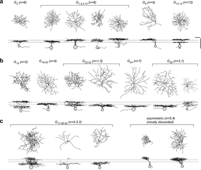
Next, we used our comparatively small sample of n=84 morphologically reconstructed cells to link functional groups to anatomically defined types. In many cases, it was possible to identify likely morphologies for functional RGC groups (Extended Data Fig. E9; SI Discussion). To generate an approximate mapping of functional groups to dendritic depth profiles in the IPL (Fig. 5), we averaged the stratification profiles of all reconstructed cells, weighted by the correlation coefficient between each cell’s light response and the functional group average (to full-field “chirp” and moving bars; Methods).

Figure 5. Mapping RGC groups to morphologies.

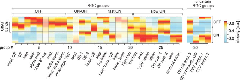
Heat map of each RGC group’s estimated dendritic stratification across the IPL (cf. Fig. 2); ON/OFF sublaminae and ChAT bands indicated. Warmer colours represent higher dendritic densities (Methods). Shaded IPL profiles indicate deviation from known stratification pattern (G₆) or an unexpected pattern given a potentially novel group’s response polarity (G_11,18,19).

The resulting map reproduced many known principles of inner retinal organisation. For example, OFF (G_1–9) and sustained ON (G_{21–24;27,28,30}) groups mostly stratified in the upper and lower half of the IPL (ref⁴) and groups with more transient responses closer to the centre (e.g. G_{1,2,8–10,20})^46,47. Most groups corresponding to known types had expected stratification profiles (e.g. W3, ON-OFF DS and classical alphas) with few exceptions (e.g. G_6,11,18,19). For example, our prediction was for the JAM-B (G₆) to stratify mainly below the ChAT-band, while the cell is known to stratify above it, as it also does in our individual examples (Extended Data Fig. E9a). This is likely caused by many cell types with responses comparable to those of the JAM-B confounding the G₆ IPL profile.

Conclusions

We found that a minimum of 32 different functional types of RGCs could be distinguished based on their light responses and basic anatomical criteria. The unusually high abundance of some of these functional types and evidence from immunohistochemistry suggests that further sub-divisions are needed. Accordingly, the number of distinct visual feature channels available to the mouse’s brain appears to be two- to threefold that of previous estimates.

Taken together, our RGC groups cover a broad range of “classical” features such as polarity, receptive field size, frequency and contrast sensitivity (Extended Data Fig. E10). In particular, RGC groups broadly span feature-dimensions such as response polarity and their preference for global vs. local stimuli. Less balanced is the temporal frequency selectivity, with only a few groups preferring high frequencies, in particular for groups with low contrast preference.

We verified our suggested functional classification by showing that most (i) functionally defined types (ii) exhibited a similar CF, (iii) some could be linked to genetically defined populations and (iv) had consistent morphology/dendritic stratification profiles in the IPL. Nonetheless, our definitions certainly remain incomplete; the classification of mouse RGCs will need to be refined by the expansion of the probed stimulus space, the use of cell-type selective genetic lines⁴⁰ or single-cell transcriptomics⁴⁸, and integration with data from large-scale EM⁴⁹. However, even our comparatively basic analysis already reveals a large diversity in feature coding by mouse RGCs, very different from how digital cameras encode images, rather resembling an encoding strategy used in state-of-the-art artificial vision systems⁵⁰. In the future, the “fingerprint” of different functional RGC types introduced here can provide a frame of reference for systematic investigations of feature coding by RGCs and for detecting functional changes in degenerated retina.

METHODS

Animals and tissue preparation

All procedures were performed in accordance with the law on animal protection issued by the German Federal Government (Tierschutzgesetz) and approved by the institutional animal welfare committee of the University of Tübingen. For all experiments, we used 4- to 8-week-old mice of either sex. In addition to C57Bl6 (wild-type) mice, we used the transgenic lines Pvalb^Cre (“PV”, JAX 008069, The Jackson Laboratory, Bar Harbor, US;⁴³), Pcp2^Cre (“Pcp2”, JAX 006207;⁴⁴) and ChAT^Cre (JAX 006410;⁵¹), cross-bred with the red fluorescence Cre-dependent reporter line Ai9:tdTomato (JAX 007905). Due to the exploratory nature of our study, we did not use randomization and blinding.

Animals were housed under a standard 12 hr day/night rhythm. For activity recordings, animals were dark-adapted for ≥1 h, then anesthetised with isoflurane (Baxter) and killed by cervical dislocation. The eyes were enucleated and hemisected in carboxygenated (95% O₂, 5% CO₂) artificial cerebral spinal fluid (ACSF) solution containing (in mM): 125 NaCl, 2.5 KCl, 2 CaCl₂, 1 MgCl₂, 1.25 NaH₂PO₄, 26 NaHCO₃, 20 glucose, and 0.5 L-glutamine (pH 7.4). Bulk electroporation of the fluorescent Ca²⁺ indicator Oregon-Green BAPTA-1 (OGB-1) into the ganglion cell layer (GCL) was carried out as described before^19,47. In brief, the retina was dissected from the eyecup, flat-mounted onto an Anodisc (#13, 0.2 um pore size, GE Healthcare, Maidstone, UK) with the GCL facing up, and placed between two 4 mm horizontal plate electrodes (CUY700P4E/L, Nepagene/Xceltis, Meckesheim, Germany). A 10 μl drop of 5 mM OGB-1 (hexapotassium salt; Life Technologies, Darmstadt, Germany) in ACSF was suspended from the upper electrode and lowered onto the retina. After application of 10–12 pulses (+9 V, 100 ms pulse width, at 1 Hz) from a pulse generator/wide-band amplifier combination (TGP110 and WA301, Thurlby handar/Farnell, Oberhaching, Germany), the tissue was moved to the recording chamber of the microscope, where it was continuously perfused with carboxygenated ACSF at ~37°C and left to recover for ~60 minutes before the recordings started. In all experiments with wild-type mice, ACSF contained ~0.1 μM Sulforhodamine-101 (SR101, Invitrogen) to reveal blood vessels and any damaged cells in the red fluorescence channel²⁰. All procedures were carried out under very dim red (>650 nm) light.

Two-photon Ca²⁺ imaging and light stimulation

We used a MOM-type two-photon microscope (designed by W. Denk, MPI, Martinsried; purchased from Sutter Instruments/Science Products, Hofheim, Germany). Design and procedures were described previously²⁰. In brief, the system was equipped with a mode-locked Ti:Sapphire laser (MaiTai-HP DeepSee, Newport Spectra-Physics, Darmstadt, Germany) tuned to 927 nm, two fluorescence detection channels for OGB-1 (HQ 510/84, AHF/Chroma Tübingen, Germany) and SR101 (HQ 630/60, AHF), and a water immersion objective (W Plan-Apochromat 20x/1,0 DIC M27, Zeiss, Oberkochen, Germany). For image acquisition, we used custom-made software (ScanM, by M. Müller, MPI, Martinsried, and T.E.) running under IGOR Pro 6.3 for Windows (Wavemetrics, Lake Oswego, OR), taking 64 × 64 pixel image sequences (7.8 frames/s) for activity scans or 512 × 512 pixel images for high-resolution morphology scans.

For light stimulation, we focused a DLP projector (K11, Acer) through the objective, fitted with band-pass-filtered light-emitting diodes (LEDs) (“green”, 578 BP 10; and “blue”, HC 405 BP 10, AHF/Croma) that roughly match the spectral sensitivity of moose M- and S-opsins. LEDs were synchronised with the microscope’s scan retrace. Stimulator intensity (as photoisomerisation rate, 10³ P*/s/cone) was calibrated as described previously⁵² to range from 0 (LEDs off) to 10.8 and 9.9 for M- and S-opsins, respectively. Due to two-photon excitation of photopigments, an additional, steady illumination component of ~10⁴ P*/s/cone was present during the recordings (for detailed discussion, see²²). For all experiments, the tissue was kept at a constant intensity level (see stimuli below) for at least 30 s after the laser scanning started before light stimuli were presented. Four types of light stimulus were used (Fig. 1b, top): (i) Full-field “chirp” stimulus consisting of a bright step and two sinusoidal intensity modulations, one with increasing frequency and one with increasing contrast, (ii) 0.3 × 1 mm bright bar moving at 1 mm/s in 8 directions¹⁹, (iii) alternating blue and green 3 s flashes, and (iv) binary dense noise, a 20×15 matrix with 40 μm pixel-side length; each pixel displayed an independent, perfectly balanced random sequence at 5 Hz yielding a total running time of 5 minutes for receptive field (RF) mapping. In some experiments, we used in addition dark moving bars (like (ii) but contrast-inversed), and stationary bright or dark 0.2 × 0.8 mm bars flashed for 1 s in 6 orientations (see Extended Data Fig. E7g–i). Except for (iii), stimuli were achromatic, with matched photo-isomerisation rates for M- and S-opsins.

Single-cell electrophysiology, dye filling and morphological reconstruction

TdTomato- or OGB-1- labelled RGCs were targeted using two-photon imaging for juxtacellular recordings using borosilicate electrodes (4–6 MΩ) filled with ACSF with added SR101 (250 μM). Data were acquired using an Axoclamp-900A or Axopatch 200A amplifier in combination with a Digidata 1440 (all: Molecular Devices, Biberach-an-der-Riss, Germany), digitised at 10 kHz and analysed off-line using IGOR Pro. We presented the same light stimuli as for the Ca²⁺ imaging. In some experiments, electrical recordings and Ca²⁺ imaging was performed simultaneously. After the recording, the membrane under the electrode was opened using a voltage “buzz” to let the cell fill with dye by diffusion for approximately 30 minutes; then 2P image stacks were acquired to document the cell’s morphology.

Filled cells were traced semi-automatically offline using the Simple Neurite Tracer plugin implemented in Fiji (http://fiji.sc/Fiji), yielding cell skeletons. If necessary, we used the original image stack to correct the skeletons for any warping of the IPL using custom-written scripts in IGOR Pro. To this end, we employed the SR101-stained blood vessel plexuses on either side of the IPL as landmarks to define the IPL borders (see below). Only cells where the filling quality allowed full anatomical reconstruction were used for analysis (see below).

Immunohistochemistry

Following Ca²⁺ imaging, retinas were mounted onto filter paper (0.8 μm pore size, Millipore) and fixed in 4% paraformaldehyde (in PBS) for 15 min at 4°C. Immunolabelling was performed using antibodies against ChAT (choline-acetyltransferase; goat anti-ChAT, 1:100, AB144P, Millipore), GAD67 (glutamate decarboxylase; mouse anti-GAD67, 1:100, MAB5046, Millipore), SMI-32 (mouse anti-SMI32, 1:100, SMI-32R-100, Covance), and melanopsin (rabbit anti-melanopsin, 1:4000, AB-N38, Advanced Targeting Systems) for 4 days. Secondary antibodies were Alexa Fluor conjugates (1:750, 16 hours, Life Technologies). For each retina, the recorded region was identified by the local blood vessel pattern and confirmed by comparing size and position of individual somata in the GCL. Image stacks were acquired on a confocal microscope (Nikon Eclipse C1) equipped with a x60 oil objective (1.4 NA). The degree of immunolabelling of GCL cells was evaluate and rated (from 0, negative, to 4 positive) using z-stacks. Attribution of labelled somata to recorded ones was performed manually using ImageJ (http://imagej.nih.gov/ij) and IGOR Pro.

Data analysis

Data analysis was performed using Matlab 2012 and 2014a (The Mathworks Inc., Ismaning, Germany), and IGOR Pro. Data were organised in a custom written schema using the DataJoint for Matlab framework (https://github.com/datajoint/datajoint-matlab; D. Yatsenko, Tolias lab, Baylor College of Medicine).

Pre-processing

Regions of interest (ROIs), corresponding to somata in the GCL, were defined semi-automatically by custom software (“CellLab” by D. Velychko, CIN) based on a high resolution (512x512 pixels) image stack of the recorded field. Then, the Ca²⁺ traces for each ROI were extracted (as ΔF/F) using the IGOR Pro-based image analysis toolbox SARFIA (http://www.igorexchange.com/project/SARFIA). A stimulus time marker embedded in the recording data served to align the Ca²⁺ traces relative to the visual stimulus with a temporal precision of 2 ms. Stimulus-aligned Ca²⁺ traces for each ROI were imported into Matlab for further analysis.

First, we de-trended the Ca²⁺ traces by high-pass filtering above ~0.1 Hz. For all stimuli except the dense noise (for RF mapping), we then subtracted the baseline (median of first 8 samples), computed the median activity r(t) across stimulus repetitions (typically 3–5 repetitions) and normalised it such that ${max}_{\mathrm{t}}(|\mathrm{r}(\mathrm{t})|)=1$.

Receptive field mapping

We mapped the linear RFs of the neurons by computing the Ca²⁺ transient-triggered average. To this end, we resampled the temporal derivative of the Ca²⁺ response $\dot{\mathit{c}}\left(t\right)$ at 10-times the stimulus frequency and used Matlab’s findpeaks function to detect the times t_i at which Ca²⁺ transients occurred. We set the minimum peak height to 1 s.d., where the s.d. was robustly estimated using:

$$\overline{\sigma }=\frac{\mathit{median}\left(\left|\dot{r}(t)\right|\right)}{0.6745}.$$

We then computed the Ca²⁺ transient-triggered average stimulus, weighting each sample by the steepness of the transient:

$$\mathit{F}(x,y,\tau )=\frac{1}{M}{{\displaystyle \sum }}_{i=1}^M\dot{\mathit{c}}(t_i)\mathit{S}\left(x,y,t_i+\tau \right)$$

Here, $\mathit{S}(x,y,t)$ is the stimulus, τ is the time lag (ranging from approx. −320 to 1,380 ms) and M is the number of Ca²⁺ events. We smoothed this raw RF estimate using a 5×5 pixel Gaussian window for each time lag separately. RF maps shown correspond to a s.d. map, where the s.d. is calculated over time lags τ:

$${\mathit{F}}_{\mathit{map}}\left(x,y\right)=SD{\left[\mathit{F}\left(x,y,\tau \right)\right]}_{\tau }$$

To extract the RF’s position and scale, we fitted it with a 2D Gaussian function using Matlab’s lsqcurvefit. The time course of the receptive field ${\mathit{F}}_{tc}(\tau )$ was estimated by the average of the 8 pixels closest to the fitted RF centre (according to the Mahalanobis distance) weighted by a Gaussian profile. RF quality (RF_qi) was measured as one minus the fraction of variance explained by the Gaussian fit ${\overline{F}}_{\mathit{map}}$,

$$Q{I}_{\mathit{RF}}=1-\frac{\mathit{Var}[F_{\mathit{map}}-{\overline{F}}_{\mathit{map}}]}{\mathit{VaI}[F_{\mathit{map}}]}.$$

Direction and orientation selectivity

To extract time course and directional tuning of the Ca²⁺ response to the moving bar stimulus, we performed a singular value decomposition (SVD) on the T by D normalised mean response matrix M (times samples by number of directions; $T=32$; $D=8$; Extended Data Fig. E7a):

$$[\mathit{U},\mathit{S},\mathit{V}]=\mathit{svd}(\mathit{M})$$

This procedure decomposes the response into a temporal component in the first column of U and a direction dependent component or tuning curve in the first column of V, such that the response matrix can be approximated as an outer product of the two:

$$\mathit{M}\approx {\mathit{S}}_{11}{\mathit{U}}_{:1}{\mathit{V}}_{:1}^T.$$

An advantage of this procedure is that it does not require manual selection of time bins for computing direction tuning, but extracts the optimal direction tuning curve given the varying temporal dynamics of different neurons.

To measure direction selectivity (DS) and its significance, we projected the tuning curve ${\mathit{V}}_{:1}$ on a complex exponential ${\varphi }_k=\text{exp}(i_k)$, where ${\alpha }_k$ is the direction in the k-th condition:

$$K={\varphi }^T{\mathit{V}}_{:1}.$$

This is mathematically equivalent to computing the vector sum in the 2D plane or computing the power in the first Fourier component. We computed a DS index as the resulting vector length

$$\mathit{DSi}=|K|,$$

correcting for the direction spacing. We additionally assessed the statistical significance of direction tuning using a permutation test⁵³. To this end, we created surrogate trials (i.e. stimulus repetitions) by shuffling the trial labels (i.e. destroying any relationship between condition and response), computed the tuning curve for each surrogate trial and projected it on the complex exponential $\varphi$. Carrying out the procedure 1,000 times generated a null distribution for K, assuming no direction tuning. We used the percentile of the true K as the p-value for direction tuning (Extended Data Fig. E7b). Importantly, a large DSi does not necessarily result in a small p-value, e.g. in the case of large trial to trial variability. As a result, the DSi distributions of significantly and not significantly direction tuned neurons show substantial overlap (Extended Data Fig. E7c,d). Therefore, a simple threshold as a DS criterion (e.g. DSi > 0.4) does not provide a good separation into direction selective cell types and others.

Orientation selectivity (OS) was assessed in an analogous way. However, we used the complex exponential ${\varphi }_k=\text{exp}(2i_k)$, corresponding to the second Fourier component.

Other response measures

Response quality index

To measure how well a cell responded to a stimulus (chirp, moving bar, colour), we computed the signal-to-noise ratio

$$QI=\frac{\mathit{Var}{\left[{\langle \mathit{C}\rangle }_r\right]}_t}{{\langle \mathit{Var}{\left[\mathit{C}\right]}_t\rangle }_r},$$

where C is the T by R response matrix (time samples by stimulus repetitions) and 〈 〉_x and $\mathit{Var}{\left[\right]}_x$ denote the mean and variance across the indicated dimension, respectively. If all trials are identical such that the mean response is a perfect representative of the response, QI is equal to 1. If all trials are completely random with fixed variance (so that the mean response is not informative about the individual trial responses at all), QI is proportional to 1/R.

For further analysis, we used only cells that responded well to the chirp and/or the moving bar stimulus ( $Q{I}_{\mathit{chirp}}>.45$ or $Q{I}_{\mathit{DS}}>0.6$).

Full-field index

The full-field index was computed as

$$\mathit{FFi}=\frac{Q{I}_{\mathit{DS}}-Q{I}_{\mathit{Chirp}}}{Q{I}_{\mathit{DS}}+Q{I}_{\mathit{Chirp}}},$$

comparing the response quality to a local stimulus (moving bar) and a global stimulus (chirp).

ON-OFF index

ON-OFF preference was measured as

$$\mathit{OOi}=\frac{{\langle r_{\mathit{ON}}\rangle }_t-{\langle r_{\mathit{OFF}}\rangle }_t}{{\langle r_{\mathit{ON}}\rangle }_t+{\langle r_{\mathit{OFF}}\rangle }_t},$$

where r_ON and r_OFF are defined as the activity during the response to the leading edge of the moving bar (the first 400 ms of the OFF response) and the trailing edge of the moving bar (the first 400 ms of the OFF response).

Colour selectivity index

Colour selectivity was measured for the ON response using

$$G{B}_{\mathit{ON}}=\frac{max(r_{\mathit{ON},\mathit{green}}^2)-max(r_{\mathit{ON},\mathit{blue}}^2)}{max(r_{\mathit{ON},\mathit{green}}^2)+max(r_{\mathit{ON},\mathit{blue}}^2)}$$

and for the OFF response using an analogous definition. Here, r_ON,green and r_ON,blue are the responses in a time window of 1,280 ms after onset of the green and blue stimulus, respectively.

Feature extraction

We used sparse principle component analysis⁵⁴, as implemented in the SpaSM toolbox by K. Sjöstrang et al. (http://www2.imm.dtu.dk/projects/spasm/), to extract sparse response features from the responses to the chirp, colour, and moving bar stimulus, resulting in features which use only a small number of time bins. The extracted features are localised in time and therefore readily interpretable (e.g. “high-frequency feature”), although this constraint was not explicitly enforced by the algorithm (Extended Data Fig. E2d₂). We also explored alternative feature extraction techniques such as regular PCA, but these resulted in inferior cluster quality. In addition, they required manually defining regions corresponding to specific parts of the stimulus (e.g. frequency chirp) to yield localised and interpretable features.

We extracted 20 features with 10 non-zero time bins from the mean response to the chirp (averaging across trials) and 6 features with 10 non-zero time bins from the mean response to the colour stimulus. For the moving bar stimulus we extracted 8 features with 5 non-zero time bins from the response time course (see above) and 4 features with 6 non-zero time bins from its temporal derivative. All features were in the temporal domain, ensuring spatial invariance. In addition, we used two features from the time course of the RF, extracted with regular PCA. Overall, this procedure resulted in a 40 dimensional feature vector for each cell. Before clustering, we standardised each feature separately across the population of cells.

Clustering

DS and non-DS cells were clustered independently, classifying cells as DS if the permutation test resulted in P<0.05. We fit each data set with a Mixture of Gaussian model using the expectation-maximisation algorithm (Matlab’s gmdistribution object). We constrained the covariance matrix for each component to be diagonal, resulting in 80 parameters per component (40 for the mean, 40 for the variances). We further regularised the covariance matrix by adding a constant (10⁻⁵) to the diagonal. To find the optimal number of clusters, we evaluated the Bayesian Information Criterion⁵⁵

$$\mathit{BIC}=-2\log L+M\log N,$$

where L is the log-likelihood of the model, N is the number of cells and M is the number of parameters in the model, i.e. $M=81C-1$, where C is the number of clusters and the contributions that arose from means, variances and mixture proportions (which have to add to 1). Although other choices such as the Aikaike information criterion (AIC) would have been possible, we found the BIC to yield a good compromise between model complexity and quality, since the AIC is known to find to many clusters for large sample sizes. We also computed log Bayes factors as $2\mathrm{\Delta }\mathit{BIC}$ for each candidate cluster number to test how strong the evidence for further splitting is. Values > 6 were treated as strong evidence in favour of further splitting. The minimum of the BIC coincided well with the number of clusters after which there was no strong evidence for further adding more clusters. To avoid local minima, we restarted the EM algorithm 20 times per candidate number of clusters and used the solution with the largest likelihood. This procedure resulted in 24 and 48 clusters for DS and non-DS cells, respectively (Extended Data Fig. E2a).

To evaluate cluster quality, we rank-ordered the posterior probabilities for cluster assignment for each cluster, normalised for cluster size and averaged across clusters for non-DS and DS cells separately (Extended Data Fig. E2b). The steep decays of the sigmoidal functions indicate good cluster separability. To check how consistent the clustering was against subsampling of the data, we created 20 surrogate datasets containing random selections of 90% of the cells. We fit these surrogate datasets with a Mixture of Gaussians model with the optimal number of clusters determined on the original dataset. For each cluster mean in these models, we computed the correlations with the most similar cluster for the model fit on the original dataset. To summarise the similarity of clusterings, we computed the median correlation across clusters (Extended Data Fig. E2c). On average, the clusterings obtained on the surrogate and the original dataset were very similar (mean median correlation: 0.96 ± 0.19 and 0.97 ± 0.01; mean ± s.d.; for DS and non-DS cells separately).

In addition, we performed an alternative clustering version, were we did not split the data in DS and non-DS cells but added DSi, OSi, soma and receptive field size as features. The identified clusters were very similar, but this strategy failed to identify most DS types as separate clusters, except for the ON-OFF DS cell. Therefore, we decided to first isolate significant DS cells and cluster them separately, before merging similarly responding DS- and non-DS clusters (see below), if we did not find a reason to keep the DS group as a separate RGC type. Nevertheless, a strategy equally justified as ours could start with the alternative clustering and then split those clusters containing significant fractions of DS cells.

Automatic identification of RGCs and ACs

A subset of cells was stained against GAD67 to identify dACs (see above). The intensity of this staining was manually rated as follows: −2 (absent), −1 (likely absent), 0 (uncertain), 1 (likely present), and 2 (present). For each cluster, we computed the average staining from the labelled cells (average number of cells with GAD67 information per cluster: 16.8± 10.0, mean ± s.d.). Clusters with an average staining <−0.2 were labelled RGCs (n=30 clusters), those with average staining >0.2 were labelled ACs (n=26). Clusters with average staining in between those values (n=5), or those that contained 6 or less cells with GAD67 information (n=8) were labelled as uncertain, unless other clear criteria such as soma size or genetic labels indicated that they are ACs or RGCs. In this case they were manually allocated to RGC or AC (n=3 and n=2, respectively). Two clusters automatically classified as AC were included in the uncertain group due to its functional similarity with the OFF-suppressed types (G₃₁). This procedure resulted in 33 RGC clusters, 10 uncertain clusters and 26 AC clusters.

Identification of alpha-RGCs

We extracted all cells with large cell bodies (>136 μm²; mean +1 s.d. of total soma size distribution; Extended Data Fig. E2g,h) from RGC and uncertain clusters. Predominantly, these cells had been assigned to nine of the clusters. We re-clustered those cells using a mixture of Gaussian model as described above, resulting in 16 clusters (Extended Data Fig. E2h). Receptive field size was not used in this process. Five of these clusters could be clearly associated with the three known alpha-RGC types and their response profiles³¹ (trans. OFF alpha, 2; sust. OFF alpha, 2; ON alpha, 1). Cells in these clusters were SMI-32-positive, as expected from alpha RGCs (Fig. 3f). Likely, this procedure missed some alpha cells, as somata close to the edge of scan fields were cut and we thus underestimate the soma size of these cells (e.g. G₅c, see also main text). Remaining cells were kept in their original cluster. Logistic regression was used to assess the effect cell type (alpha vs. mini) on SMI-32 staining (absent vs. present). We used the Matlab implementation fitglm with a binomial non-linearity. 95%-confidence intervals on the proportion of SMI32-positive cells were computed using bootstrapping with 1,000 samples.

Dendrogram

We used a standard linkage algorithm on the means of the RGC groups in the standardised feature space with correlation distance $d_{ij}=1-\mathit{corr}(m_i,m_j)$ and average unweighted distance and plotted the result as a dendrogram (using Matlab functions linkage and dendrogram). The leaf order was optimised using the Matlab function optimalleaforder and modified for clarity of presentation.

Calculation of coverage factor

We calculated each group’s coverage factor (CF),

$$CF=\frac{n_{\mathit{Cells}}\ast A_{RF,\mathit{median}}}{A_{\mathit{Scan}}}$$

with the number of cells in a group ( $n_{\mathit{Cells}}$), the median RF size ( $A_{RF,\mathit{median}}$) within a group counting only cells that surpassed a RF quality criterion of 0.3, and the total scan area across all experiments ( $A_{\mathit{Scan}}$). We corrected $n_{\mathit{Cells}}$ for 29% cells discarded by our quality criterion as well as an empirically estimated 8% of cells that did not yield a ROI in the first place due to weak or absent labelling. In addition, $A_{\mathit{Scan}}$ was corrected for an empirically estimated 34.8% RF overhang (=where a cell’s RF exceeds the scan field edge. This procedure yielded a CF 2.0 ± 0.7 for most RGC groups (Gaussian fit; see Fig. 2e, right). However, differences between studies in approaches to measure RFs (e.g. checkerboards vs. bars), in the assumptions used for RF fitting (e.g. homogenous RFs best fitted by Gaussians), or in the methods to estimate dendritic arbour area can easily yield different absolute estimates of CF (cf. also SI Table 1).

Estimation of IPL stratification profiles

To determine a cell’s IPL stratification profile, we calculated dendritic density as described previously¹⁰ with spatial smoothing of 1 μm³. The resultant 3D density-cloud was projected on the Z-axis to estimate the mean IPL depth profile. The relationship between the depth profiles and the two ChAT bands was estimated in independent experiments using mice that express tdTomato in cholinergic ACs (ChAT^Cre × Ai9:tdTomato). We compared the IPL depth of the tdTomato-labelled dendritic plexi to the two SR101-labelled blood vessel planes that line the inner retina. We estimated the error to be ~1.5 μm (s.d.), corresponding to 3–4% IPL depth (n=13 measurements in 2 mice).

To relate each cell’s IPL profile to functional groups we calculated the mean correlation coefficient between a cell’s response to the “chirp” and moving bar stimuli and each group’s mean response. The correlation coefficient (−1…1) for each pair was then multiplied with the cell’s depth profile and a correlation-rank based weighting factor $W={0.9}^{\mathit{rank}-1}$. Thus, each individual recording yielded a complete two-dimensional map, with IPL depth on one axis and functional group on the other. Next, we averaged across the maps for those cells that passed our response quality criterion (n_(non-DS) = 31/51; n_(DS) = 24/33; see above). The resultant matrices were normalised in two steps: First, we divided each group’s IPL depth profile by the mean depth profile of all included cells to eliminate any bias in sampling depth. Second, we divided each depth profile by its own maximum. This resulted in an automatic and unbiased estimate of dendritic stratification depth for all RGC groups (Fig. 5). Note that this automated approach is based on a relatively small sample of reconstructed cells and therefore can only provide an approximate prediction of stratification levels. Notably, this approach is invariant to differences in lateral dendritic field dimensions that may be associated with retinal position (e.g.^10,23).

Extended Data

Figure E1. Linking electrophysiology and imaging data (related to Fig. 1).

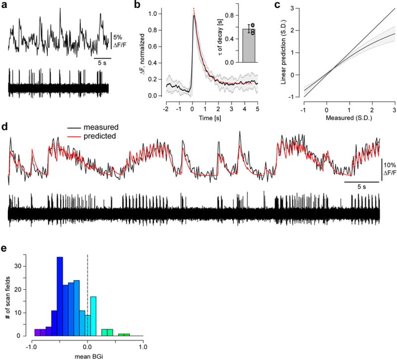
a, simultaneously recorded RGC Ca²⁺ (top) and spiking (bottom) activity in response to binary spatial dense noise stimulation. b, average Ca²⁺ event triggered by a single spike, averaged across n=6 cells (shading = 1 s.d.); event decay was fit (red) using a single exponential (for time constant τ, see inset, mean ± 1 s.d.) to yield an estimated impulse response. A linear prediction of Ca²⁺ (calculated by convolution of the impulse response with binarised spike-traces) was compared to measured values to estimate the mean nonlinearity (c). d, Ca²⁺ (top) and spiking (bottom) response to the full-field “chirp” stimulus (Methods) simultaneously recorded in an RGC (red trace, Ca²⁺ signal predicted from spiking response). e, number of scan fields as a function of blue-green index (BGi, see Methods) averaged over all ROIs in each field (cf. Fig. 1a₁).

Figure E2. Clustering and grouping (related to Fig. 2).

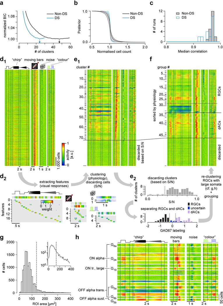
a–c. Selection of cluster size and cluster quality/consistency analysis. a, normalised Bayesian Information Criterion (BIC) curves for non-DS (black) and DS (blue) cells. Arrows indicate the optimal numbers of clusters. b, rank-ordered posterior probability curves indicating cluster quality. Curves were normalised for cluster size and averaged for non-DS (black) and DS (blue) clusters separately. Shaded area indicates 1 s.d. across clusters. c, histogram of median correlation between the original clusters and clusters identified on 20 surrogate datasets, created by repeated subsampling of 90% of the original dataset (bootstrapping); for each cluster, the best matching cluster from the original clustering was selected. d, heat maps of Ca²⁺ responses (d₁) to the 4 visual stimuli (cf. Fig. 1) of n=11,210 cells from 50 retinas. Shown are raw data sorted by the response to the colour stimulus. Each line represents responses of a single cell with activity colour-coded such that warmer colours represent increased activity. Temporal features (d₂) were extracted from the cells’ light responses (Methods) and used for automatic clustering (d₁ → e₁). e, heat maps showing clustered data (e₁, n=72 clusters plus cells discarded based on signal-to-noise (S/N) ratio), with block height representing the number of included cells. Distributions of S/N (e₂, top) and GAD67 labelling (e₂, bottom) used to discard clusters and sort the remaining ones into retinal ganglion cells (RGCs), “uncertain” RGCs and displaced amacrine cells (dACs). f, heat maps showing n=46 groups (divided into n=32 RGC groups, including n=4 “uncertain” ones, and n=14 dAC groups; sorted by response similarities) after re-clustering of large-soma cells (alpha cell post-processing, see panels g,h). g, distribution of region of interest (ROI) area (as proxy for soma size) for all cells classified as RGCs and “uncertain” (e₂). Inset: same distribution but on a log-scale. Dashed line marks threshold to separating large-soma cells (Methods). h, results of re-clustering of large-soma cells (from g): heat maps show light-evoked Ca²⁺ responses to the 4 visual stimuli (cf. Fig. 1b). Clusters that resulted in new RGC groups are indicated; the remaining cells stayed with their original clusters.

Figure E3. Group overview – Functional groups classified as “uncertain” RGCs and displaced amacrine cell (dAC) in the mouse retina (related to Fig. 2).

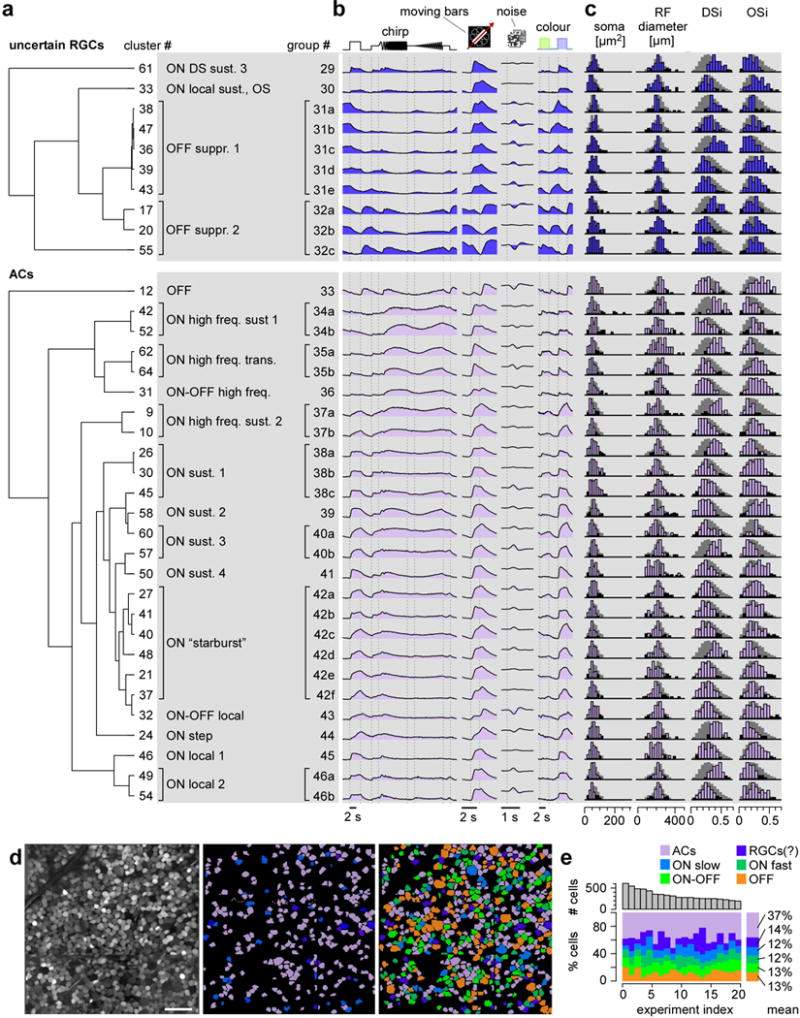
a, clusters organised according to hierarchical trees (dendrograms, see Methods) and grouped based on functional similarity (see main text for details), resulting in n=4 “uncertain” RGC (top) and n=14 dAC groups (bottom). b, mean Ca²⁺ responses to the 4 stimuli (cf. Fig. 1b) for each cluster. c, histograms of selected properties, from left to right: ROI (soma) area, receptive field (RF) diameter (2 s.d. from Gaussian fit; see Fig. 1b₁ and Fig. E4), DS and OS indices (DSi and OSi, respectively, Methods). For details on each cluster, see also SI Data 1_40–49 (“uncertain”), and SI Data 1_50–75 (dACs). d, example experiment (left, from Fig. 1a₂); centre: showing dACs (lilac) and “uncertain” RGCs (blue); right: colour-coded by broad categories, as in (e). e, total number of cells (top) and percentage of cells in sets of groups (bottom) per experiment (only experiments with ≥198 cells) illustrating consistency across experiments. Scale bar: d, 50 μm.

Figure E4. Relationship between RGC receptive field centres and their dendritic arbours (related to Fig. 2).

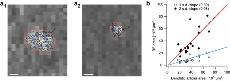
a, receptive field (RF) centre maps of a G₈ transient OFF alpha RGC (a₁) and a G₂ small-field RGC (a₂), with their reconstructed morphologies overlaid. 1- and 2-s.d. contours of RF centres fitted with 2D Gaussians are indicated by blue and red ovals, respectively. b, area of RF centre fits from (a) as function of dendritic arbour area (n=18 RGCs). Scale bar: 100 μm.

Figure E5. Mapping RGC groups onto genetic types – Functional diversity of PV- and Pcp2-positive RGCs (related to Fig. 2).

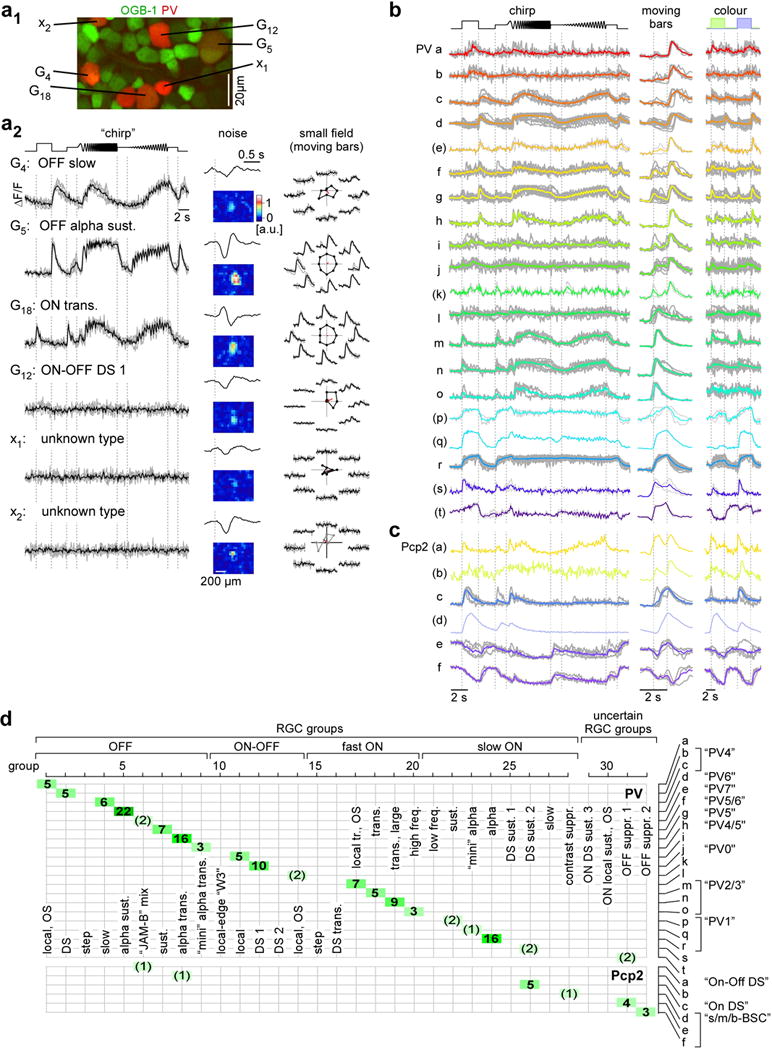
a, diversity of PV-positive RGCs (red) in a PV:tdTomato mouse retina electroporated with OGB-1 (a₁, green). Ca²⁺ responses and receptive fields (a₂) from 6 PV-positive cells in exemplary field are shown (black, mean response, grey, single trials). The top four cells could be clearly matched to RGC groups (cf. Fig. 2), whereas the remaining two (x₁, x₂) were discarded due to the lack of responses to both full-field and moving bar stimuli; note, however that both cells yielded a clear RF. b, Ca²⁺ responses of functionally distinct PV-RGC groups (20 response types PV a-t, thereof 14 with n ≥ 3 cells). Traces colour-coded by group assignment (colours as in Fig. 2) represent mean responses, with individual cell responses in grey. c, same for Pcp2-positive (6 response types Pcp2 a-f, thereof 3 with n ≥ 3 cells) RGC groups. d, table illustrating the relationship between RGC groups (Fig. 2) and functional PV- and Pcp2-positive RGC types from (a,b). Numbers represent the total cell count of each allocation. Names in quotes (e.g. “PV5”) refer to the cells’ original names (see PV-⁴⁵ and Pcp2-study⁵⁶).

Figure E6. Examples of RGC groups.

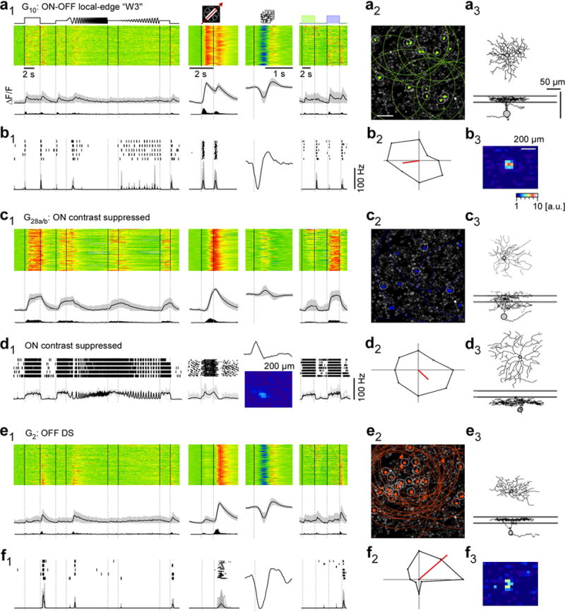
a, functional “fingerprint” of G₁₀ RGCs, identified as local-edge-detector (W3) cells. Light-evoked Ca²⁺ responses of n=149 cells (a₁): heat maps (top) illustrating individual responses, with response averages and firing rates estimated from Ca²⁺ signals (cf. Fig. E1a–d) below. Ganglion cell layer (a₂; experiment from Fig. 1a₂) with G₁₀ somata (green) and receptive fields (RFs, dotted) indicated. Grey circles mark cells with RFs that passed a quality criterion (Methods). Example morphology of a G₁₀ cell filled after electrical single-cell recording (a₃, cf. b). For a complete summary of the group’s properties, see SI Data 2₁₀. b, electrical single-cell recording of a G₁₀ cell: spiking responses as raster plots and mean spike rates for “chirp”, moving bar and blue/green stimuli as well as time kernel derived from noise stimulus (b₁), polar plot of responses to moving bar (b₂) and RF map (b₃) c_1,2, G_28a,b (n=100) contrast-suppressed ON RGCs with sample morphology (c₃; G_28a,b cell dye-injected after Ca²⁺ imaging). d_1,2, electrical single-cell recording of a contrast-suppressed ON RGC with different morphology (d₃ vs. c₃). e,f, G₂ direction-selective OFF RGCs (n=162) that stratify between the ChAT bands (e₃), as fingerprint (e_1,2) and exemplary electrical single-cell recording (f_1–3). Scale bars: 50 μm; grey lines in a₃,c₃,d₃,e₃: ChAT bands.

Figure E7. Direction and orientation selectivity (related to Fig. 4).

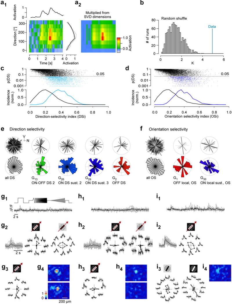
a, (a₁) stimulus direction vs. time map for an exemplary direction selective RGC with temporal (top) and directional (right) activation profiles shown; Singular Value Decomposition (SVD) was used to estimate the time-course and tuning function; individual stimulus repeats in grey, average in black. (a₂) Reconstruction of direction vs. time map based on time course and tuning function of extracted by SVD. b, statistical significance testing for direction selectivity (DS) or orientation selectivity (OS) was performed by projecting the direction/orientation profile on a single (for DS) or double (for OS) period cosine (blue) and the magnitude of the projection to the distribution of projections obtained by randomly permuting tuning-angles from the original data (grey; bootstrapping). The p-value is obtained by computing the percentile of the data (blue) in the bootstrap distribution (grey). c, d, p-values for direction (c) and orientation (d) tuning as function of the respective selectivity index (top, scatter plot; bottom, histogram; black, non-DS cells; light blue, DS cells; dark blue, OS cells). Note that tuning probability (p_DS, p_OS) only partially predicted tuning strength (DSi, OSi). e, pairs of polar plots showing the distribution of preferred motion directions for all direction-selective (DS) RGCs together and for all DS RGC groups not shown in Fig. 4, (V, ventral; N, nasal direction; same group colour code as in Fig. 2). Top plot of each pair: the cells’ individual preferred directions, with line length representing DSi and line grey level p(DS) (Methods). Bottom plot of each pair: circular histogram of preferred direction. f, like (a) but for orientation-selective (OS) RGCs. g–i, exemplary OS RGCs, illustrating the functional diversity within G₁₇ (local ON trans. OS cells); none of them display strong full-field responses (g₁,h₁,i₁, left). A “vertically-tuned” ON OS cell (g₂, left) that shows little tuning to a dark moving bar (g₂, right; g₃, another example). Note the lobular structures bracketing the RF centre (coloured RF maps in g₄). Two examples for “horizontally-tuned” ON OS cells (h_2,3) with their respective RF maps (h₄). ON OS cell that shows weak tuning to bright moving bars (i₁, left) but strong OS to stationary bright and dark bars (i_2–4, centre and right, respectively; Methods).

Figure E8. Retinal distribution of PV-positive cells in the PV^Cre × Ai9^tdTomato mouse line (related to Fig. 2).

a,b, density map (a) and magnified sample areas (b) illustrate PV-labelling anisotropy.

Figure E9. Mapping RGC groups to morphologies.

a–c, exemplary morphologies of RGCs filled after electrical recording or Ca²⁺ imaging and subsequently clustered/sorted into specific RGC groups or discarded (c, right) based on their light response S/N. Scale bars: 50 μm.

Figure E10. RGC groups cover a basic feature space.

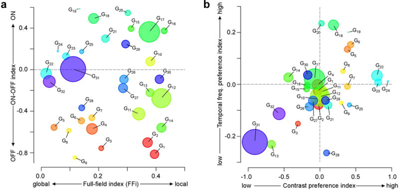
a,b, relationship of four basic response indices of RGC groups. Disc-area shows group size. Indices capture preference for stimulus polarity (ON-OFF index; Methods), for high vs. low temporal frequencies and contrasts (see below), as well as the full-field index (FFi; Methods), which reflects response preference for global (full-field “chirp”) versus local (moving-bar) stimulation. Contrast- and Frequency-indices represent contrasts of feature activation ( $\left(F_j-F_k\right)/\left(F_j+F_k\right)$) at respective time points during the full-field “chirp” stimulus, with j=12, k=9 for frequency, and j=17, k=15 for contrast. Before calculating ratios, feature activation (F) was normalised (0…1) by passing values through a cumulative normal distribution.

References

- 1.Masland RH. The neuronal organization of the retina. Neuron. 2012;76:266–280. doi: 10.1016/j.neuron.2012.10.002. [DOI] [PMC free article] [PubMed] [Google Scholar]
- 2.Euler T, Haverkamp S, Schubert T, Baden T. Retinal bipolar cells: elementary building blocks of vision. Nat Rev Neurosci. 2014;15:507–19. doi: 10.1038/nrn3783. [DOI] [PubMed] [Google Scholar]
- 3.Lettvin J, Maturana H, McCulloch W, Pitts W. What the Frog’s Eye Tells the Frog’s Brain. Proc IRE. 1959;47:1940–1951. [Google Scholar]
- 4.Werblin FS, Dowling JE. Organization of the retina of the mudpuppy, Necturus maculosus. II Intracellular recording. J Neurophysiol. 1969;32:339–355. doi: 10.1152/jn.1969.32.3.339. [DOI] [PubMed] [Google Scholar]
- 5.Cleland BG, Levick WR. Brisk and sluggish concentrically organized ganglion cells in the cat’s retina. J Physiol. 1974;240:421–456. doi: 10.1113/jphysiol.1974.sp010617. [DOI] [PMC free article] [PubMed] [Google Scholar]
- 6.Barlow HB, Hill RM, Levick WR. Rabbit retinal ganglion cells responding selectively to direction and speed of image motion in the rabbit. J Physiol. 1964;173:377–407. doi: 10.1113/jphysiol.1964.sp007463. [DOI] [PMC free article] [PubMed] [Google Scholar]
- 7.Devries SH, Baylor DA. Mosaic arrangement of ganglion cell receptive fields in rabbit retina. J Neurophysiol. 1997;78:2048–2060. doi: 10.1152/jn.1997.78.4.2048. [DOI] [PubMed] [Google Scholar]
- 8.Farrow K, Masland RH. Physiological clustering of visual channels in the mouse retina. J Neurophysiol. 2011;105:1516–30. doi: 10.1152/jn.00331.2010. [DOI] [PMC free article] [PubMed] [Google Scholar]
- 9.Coombs J, van der List D, Wang GY, Chalupa LM. Morphological properties of mouse retinal ganglion cells. Neuroscience. 2006;140:123–36. doi: 10.1016/j.neuroscience.2006.02.079. [DOI] [PubMed] [Google Scholar]
- 10.Sümbül U, et al. A genetic and computational approach to structurally classify neuronal types. Nat Commun. 2014;5:3512. doi: 10.1038/ncomms4512. [DOI] [PMC free article] [PubMed] [Google Scholar]
- 11.Völgyi B, Chheda S, Bloomfield SA. Tracer coupling patterns of the ganglion cell subtypes in the mouse retina. J Comp Neurol. 2009;512:664–87. doi: 10.1002/cne.21912. [DOI] [PMC free article] [PubMed] [Google Scholar]
- 12.Kong JH, Fish DR, Rockhill RL, Masland RH. Diversity of ganglion cells in the mouse retina: unsupervised morphological classification and its limits. J Comp Neurol. 2005;489:293–310. doi: 10.1002/cne.20631. [DOI] [PubMed] [Google Scholar]
- 13.Rowe MH, Stone J. Naming of neurones. Classification and naming of cat retinal ganglion cells. Brain Behav Evol. 1977;14:185–216. doi: 10.1159/000125660. [DOI] [PubMed] [Google Scholar]
- 14.Seung HS, Sümbül U. Neuronal Cell Types and Connectivity: Lessons from the Retina. Neuron. 2014;83:1262–1272. doi: 10.1016/j.neuron.2014.08.054. [DOI] [PMC free article] [PubMed] [Google Scholar]
- 15.Sanes JR, Masland RH. The Types of Retinal Ganglion Cells: Current Status and Implications for Neuronal Classification. Annu Rev Neurosci. 2015;38:221–46. doi: 10.1146/annurev-neuro-071714-034120. [DOI] [PubMed] [Google Scholar]
- 16.Rodieck RW, Brening RK. Retinal ganglion cells: properties, types, genera, pathways and trans-species comparisons. Brain Behav Evol. 1983;23:121–64. doi: 10.1159/000121492. [DOI] [PubMed] [Google Scholar]
- 17.Robles E, Laurell E, Baier H. The Retinal Projectome Reveals Brain-Area-Specific Visual Representations Generated by Ganglion Cell Diversity. Curr Biol. 2014;24:2085–96. doi: 10.1016/j.cub.2014.07.080. [DOI] [PubMed] [Google Scholar]
- 18.Morin LP, Studholme KM. Retinofugal projections in the mouse. J Comp Neurol. 2014;522:3733–53. doi: 10.1002/cne.23635. [DOI] [PMC free article] [PubMed] [Google Scholar]
- 19.Briggman KL, Euler T. Bulk electroporation and population calcium imaging in the adult mammalian retina. J Neurophysiol. 2011;105:2601–2609. doi: 10.1152/jn.00722.2010. [DOI] [PubMed] [Google Scholar]
- 20.Euler T, et al. Eyecup scope-optical recordings of light stimulus-evoked fluorescence signals in the retina. Pflugers Arch. 2008;457:1393–1414. doi: 10.1007/s00424-008-0603-5. [DOI] [PMC free article] [PubMed] [Google Scholar]
- 21.Wang YV, Weick M, Demb B. Spectral and temporal sensitivity of cone-mediated responses in mouse retinal ganglion cells. J Neurosci. 2011;31:7670–7681. doi: 10.1523/JNEUROSCI.0629-11.2011. [DOI] [PMC free article] [PubMed] [Google Scholar]
- 22.Baden T, et al. A tale of two retinal domains: near-optimal sampling of achromatic contrasts in natural scenes through asymmetric photoreceptor distribution. Neuron. 2013;80:1206–1217. doi: 10.1016/j.neuron.2013.09.030. [DOI] [PubMed] [Google Scholar]
- 23.Bleckert A, Schwartz GW, Turner MH, Rieke F, Wong ROL. Visual space is represented by nonmatching topographies of distinct mouse retinal ganglion cell types. Curr Biol. 2014;24:310–5. doi: 10.1016/j.cub.2013.12.020. [DOI] [PMC free article] [PubMed] [Google Scholar]
- 24.Kim IJ, Zhang Y, Yamagata M, Meister M, Sanes JR. Molecular identification of a retinal cell type that responds to upward motion. Nature. 2008;452:478–482. doi: 10.1038/nature06739. [DOI] [PubMed] [Google Scholar]
- 25.Zhang Y, Kim IJ, Sanes JR, Meister M. The most numerous ganglion cell type of the mouse retina is a selective feature detector. Proc Natl Acad Sci U S A. 2012;109:E2391–8. doi: 10.1073/pnas.1211547109. [DOI] [PMC free article] [PubMed] [Google Scholar]
- 26.Schlamp CL, et al. Evaluation of the percentage of ganglion cells in the ganglion cell layer of the rodent retina. Mol Vis. 2013;19:1387–96. [PMC free article] [PubMed] [Google Scholar]
- 27.Berson DM, Castrucci AM, Provencio I. Morphology and mosaics of melanopsin-expressing retinal ganglion cell types in mice. J Comp Neurol. 2010;518:2405–22. doi: 10.1002/cne.22381. [DOI] [PMC free article] [PubMed] [Google Scholar]
- 28.Ecker JL, et al. Melanopsin-expressing retinal ganglion-cell photoreceptors: Cellular diversity and role in pattern vision. Neuron. 2010;67:49–60. doi: 10.1016/j.neuron.2010.05.023. [DOI] [PMC free article] [PubMed] [Google Scholar]
- 29.Lim EJ, Kim IB, Oh SJ, Chun MH. Identification and characterization of SMI32-immunoreactive amacrine cells in the mouse retina. Neurosci Lett. 2007;424:199–202. doi: 10.1016/j.neulet.2007.07.046. [DOI] [PubMed] [Google Scholar]
- 30.Armañanzas R, Ascoli GA. Towards the automatic classification of neurons. Trends Neurosci. 2015;38:307–318. doi: 10.1016/j.tins.2015.02.004. [DOI] [PMC free article] [PubMed] [Google Scholar]
- 31.Van Wyk M, Wässle H, Taylor WR. Receptive field properties of ON- and OFF-ganglion cells in the mouse retina. Vis Neurosci. 2009;26:297–308. doi: 10.1017/S0952523809990137. [DOI] [PMC free article] [PubMed] [Google Scholar]
- 32.Weng S, Sun W, He S. Identification of ON-OFF direction-selective ganglion cells in the mouse retina. J Physiol. 2005;562:915–923. doi: 10.1113/jphysiol.2004.076695. [DOI] [PMC free article] [PubMed] [Google Scholar]
- 33.Sun W, Deng Q, Levick WR, He S. ON direction-selective ganglion cells in the mouse retina. J Physiol. 2006;576:197–202. doi: 10.1113/jphysiol.2006.115857. [DOI] [PMC free article] [PubMed] [Google Scholar]
- 34.Tien NW, Pearson JT, Heller CR, Demas J, Kerschensteiner D. Genetically Identified Suppressed-by-Contrast Retinal Ganglion Cells Reliably Signal Self-Generated Visual Stimuli. J Neurosci. 2015;35:10815–10820. doi: 10.1523/JNEUROSCI.1521-15.2015. [DOI] [PMC free article] [PubMed] [Google Scholar]
- 35.Oyster CW, Barlow HB. Direction-selective units in rabbit retina: distribution of preferred directions. Science (80-) 1967;155:841–2. doi: 10.1126/science.155.3764.841. [DOI] [PubMed] [Google Scholar]
- 36.Levick WR. Receptive fields and trigger features of ganglion cells in the visual streak of the rabbits retina. J Physiol. 1967;188:285–307. doi: 10.1113/jphysiol.1967.sp008140. [DOI] [PMC free article] [PubMed] [Google Scholar]
- 37.Sivyer B, Taylor WR, Vaney DI. Uniformity detector retinal ganglion cells fire complex spikes and receive only light-evoked inhibition. Proc Natl Acad Sci U S A. 2010;107:5628–5633. doi: 10.1073/pnas.0909621107. [DOI] [PMC free article] [PubMed] [Google Scholar]
- 38.Nikolaev A, Leung KM, Odermatt B, Lagnado L. Synaptic mechanisms of adaptation and sensitization in the retina. Nat Neurosci. 2013;16:934–941. doi: 10.1038/nn.3408. [DOI] [PMC free article] [PubMed] [Google Scholar]
- 39.Vaney DI, Sivyer B, Taylor WR. Direction selectivity in the retina: symmetry and asymmetry in structure and function. Nat Rev Neurosci. 2012;13:194–208. doi: 10.1038/nrn3165. [DOI] [PubMed] [Google Scholar]
- 40.Rivlin-Etzion M, et al. Transgenic mice reveal unexpected diversity of on-off direction-selective retinal ganglion cell subtypes and brain structures involved in motion processing. J Neurosci. 2011;31:8760–9. doi: 10.1523/JNEUROSCI.0564-11.2011. [DOI] [PMC free article] [PubMed] [Google Scholar]
- 41.Zhao X, Chen H, Liu X, Cang J. Orientation-selective responses in the mouse lateral geniculate nucleus. J Neurosci. 2013;33:12751–63. doi: 10.1523/JNEUROSCI.0095-13.2013. [DOI] [PMC free article] [PubMed] [Google Scholar]
- 42.Feinberg EH, Meister M. Orientation columns in the mouse superior colliculus. Nature. 2014 doi: 10.1038/nature14103. [DOI] [PubMed] [Google Scholar]
- 43.Hippenmeyer S, et al. A developmental switch in the response of DRG neurons to ETS transcription factor signaling. PLoS Biol. 2005;3:e159. doi: 10.1371/journal.pbio.0030159. [DOI] [PMC free article] [PubMed] [Google Scholar]
- 44.Lewis PM, Gritli-Linde A, Smeyne R, Kottmann A, McMahon AP. Sonic hedgehog signaling is required for expansion of granule neuron precursors and patterning of the mouse cerebellum. Dev Biol. 2004;270:393–410. doi: 10.1016/j.ydbio.2004.03.007. [DOI] [PubMed] [Google Scholar]
- 45.Farrow K, et al. Ambient illumination toggles a neuronal circuit switch in the retina and visual perception at cone threshold. Neuron. 2013;78:325–338. doi: 10.1016/j.neuron.2013.02.014. [DOI] [PubMed] [Google Scholar]
- 46.Roska B, Werblin F. Vertical interactions across ten parallel, stacked representations in the mammalian retina. Nature. 2001;410:583–587. doi: 10.1038/35069068. [DOI] [PubMed] [Google Scholar]
- 47.Baden T, Berens P, Bethge M, Euler T. Spikes in mammalian bipolar cells support temporal layering of the inner retina. Curr Biol. 2013;23:48–52. doi: 10.1016/j.cub.2012.11.006. [DOI] [PubMed] [Google Scholar]
- 48.Macosko EZ, et al. Highly Parallel Genome-wide Expression Profiling of Individual Cells Using Nanoliter Droplets. Cell. 2015;161:1202–1214. doi: 10.1016/j.cell.2015.05.002. [DOI] [PMC free article] [PubMed] [Google Scholar]
- 49.Denk W, Horstmann H. Serial block-face scanning electron microscopy to reconstruct three-dimensional tissue nanostructure. PLoS Biol. 2004;2:e329. doi: 10.1371/journal.pbio.0020329. [DOI] [PMC free article] [PubMed] [Google Scholar]
- 50.Krizhevsky A, Sutskever I, Hinton GE. ImageNet Classification with Deep Convolutional Neural Networks. Adv Neural Inf Process Syst. 2012:1–9. [Google Scholar]
- 51.Rossi J, et al. Melanocortin-4 receptors expressed by cholinergic neurons regulate energy balance and glucose homeostasis. Cell Metab. 2011;13:195–204. doi: 10.1016/j.cmet.2011.01.010. [DOI] [PMC free article] [PubMed] [Google Scholar]
- 52.Breuninger T, Puller C, Haverkamp S, Euler T. Chromatic bipolar cell pathways in the mouse retina. J Neurosci. 2011;31:6504–6517. doi: 10.1523/JNEUROSCI.0616-11.2011. [DOI] [PMC free article] [PubMed] [Google Scholar]
- 53.Ecker ASS, et al. State Dependence of Noise Correlations in Macaque Primary Visual Cortex. Neuron. 2014;82:235–248. doi: 10.1016/j.neuron.2014.02.006. [DOI] [PMC free article] [PubMed] [Google Scholar]
- 54.Zou H, Hastie T, Tibshirani R. Sparse Principal Component Analysis. J Comput Graph Stat. 2006;15:265–286. [Google Scholar]
- 55.Fraley C, Raftery A. Model-based clustering, discriminant analysis, and density estimation. J Am Stat. 2002;97:611–631. [Google Scholar]
- 56.Ivanova E, Hwang GS, Pan ZH. Characterization of transgenic mouse lines expressing Cre recombinase in the retina. Neuroscience. 2010;165:233–243. doi: 10.1016/j.neuroscience.2009.10.021. [DOI] [PMC free article] [PubMed] [Google Scholar]
Associated Data
This section collects any data citations, data availability statements, or supplementary materials included in this article.