methylFlow: cell-specific methylation pattern reconstruction from high-throughput bisulfite-converted DNA sequencing

Abstract

Motivation: DNA methylation aberrations are now known to, almost universally, accompany the initiation and progression of cancers. In particular, the colon cancer epigenome contains specific genomic regions that, along with differences in methylation levels with respect to normal colon tissue, also show increased epigenetic and gene expression heterogeneity at the population level, i.e. across tumor samples, in comparison with other regions in the genome. Tumors are highly heterogeneous at the clonal level as well, and the relationship between clonal and population heterogeneity is poorly understood.

Results: We present an approach that uses sequencing reads from high-throughput sequencing of bisulfite-converted DNA to reconstruct heterogeneous cell populations by assembling cell-specific methylation patterns. Our methodology is based on the solution of a specific class of minimum cost network flow problems. We use our methods to analyze the relationship between clonal heterogeneity and population heterogeneity in high-coverage data from multiple samples of colon tumor and matched normal tissues.

Availability and implementation: http://github.com/hcorrada/methylFlow.

Contact: hcorrada@umiacs.umd.edu

Supplementary information: Supplementary information is available at Bioinformatics online.

1 Introduction

DNA methylation (DNAm) is a gene regulatory mechanism where silencing of gene expression is established by the chemical bond of methyl groups to DNA at specific genomic regions (Holliday and Pugh, 1975). It is the best understood heritable mechanism for gene regulation that does not involve direct modification of DNA sequence itself. High-throughput sequencing of bisulfite-converted DNA is used to measure DNAm modifications at base-pair level. This approach has led to deeper understanding of the methylome’s organization and its role in development (Lister et al., 2009) and disease (Hansen et al., 2011).

While single-cell methods to sequence bisulfite-converted DNA are currently under development (Smallwood et al., 2014), the most reliable current method to measure DNAm at the base-pair level across the entire methylome is to bisulfite-convert and sequence DNA from a population of cells. A number of existing computational methods may then be used to calculate the percentage of DNA fragments that harbor a DNAm modification at specific genomic loci (Hansen et al., 2012). In many normal human tissues, for example, these percentages vary from the expected levels in a population of diploid cells with identical DNAm modifications: 100% (where all cells in the population are methylated at a specific locus), 0% (where all cells in the population are unmethylated) or 50% (where only one chromosome in all cells in the population are methylated). For example, in the normal colon methylome, the majority of the methylome is partially methylated at a level of roughly 70–80% (Hansen et al., 2011). Similar patterns are observed in other human tissues (Timp et al., 2014), and tissues in other eukaryotes.

An obvious observation that follows from this is that cell populations in normal tissues are composed of epigenetically heterogenous cells. Furthermore, when comparing DNAm across different tissues, for example, colon normal tissue and colon tumor, Figure 1, or a population of stem cells to a population of somatic cells, e.g. fibroblast (Lister et al., 2009), differences in DNAm percentages at a specific locus is indicative of a shift in the epigenetic composition of these cell populations.

Fig. 1.

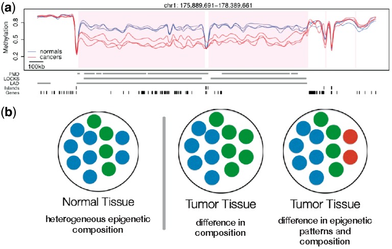
Differences in DNAm percentage at a given locus are indicative of a shift in the epigenetic composition of cell populations. (a) Base-pair-level DNAm percentage estimate for three colon tumors and paired normal tissue (Figure from Hansen et al., 2011). (b) Different shifts in the epigenetic composition of the cell population in a tissue lead to identical marginal differences of DNAm percentage at the base-pair level

Computational and statistical methods to study the epigenetic composition of cell populations have been proposed based on the analysis of DNAm modifications at multiple consecutive genomic loci spanned by single sequencing reads (Landan et al., 2012), where they analyzed DNAm modifications at each group of four contiguous CpG dinucleotides using sequencing reads that span all four CpGs. They then calculate the proportion of reads compatible with each of the 2⁴ possible DNAm modifications over these four positions. They summarize these 2⁴ proportions to define the epipolymorphism of each set of four contiguous CpGs.

While these approaches have yielded great insight into how cell populations differ epigenetically across different tissues, they only provide a general summary of the epigenetic composition of these cell populations. For instance, distinguishing between the two types of cell population shifts illustrated in 1 is limited to those differences observed over four contiguous CpGs. To perform a comprehensive analysis of these cell population shifts, the ability to reconstruct cell-specific methylation patterns over longer genomic spans is required.

In this article, we present methylFlow, a novel computational method to reconstruct cell-specific patterns using reads obtained from sequencing bisulfite-converted DNA based on network flow algorithms. We report on a simulation study characterizing the behavior of our method. We then present an application of this method using ultra-high coverage targeted sequence in a colon cancer study (Hansen et al., 2011), and on whole genome sequencing of fully differentiated B-cells and KSL and CLP progenitor cells (Kieffer-Kwon et al., 2013). We also perform a validation study using bisulfite-converted DNA from single cells (Smallwood et al., 2014). We believe that this method will allow for increased understanding of the role of epigenetic heterogeneity at the cell population level in gene regulation.

2 Methods

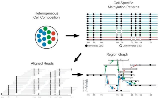
Our method uses sequencing reads from bisulfite-converted DNA to reconstruct heterogeneous cell populations by assembling cell type-specific methylation patterns spanning multiple CpGs from read overlaps (Fig. 2). It jointly reconstructs these methylation patterns and quantifies their abundance in heterogenous cell populations.

Fig. 2.

Overview of methylation pattern estimation: We assume that samples are obtained from cell populations (top left) that are epigenetically heterogeneous as determined by distinct CpG methylation patterns along a genomic region (top right). Reconstruction is based on the overlap of bisulfite converted reads to a reference genome (bottom left). Read overlaps and methylation calls are used to define a region graph (bottom right). Based on coverage (the number of reads originating in each region), a minimum cost network flow problem to estimate the number and abundance of methylation patterns (paths in the graph)

2.1 Problem formulation

Our method assumes a set of aligned reads from a bisulfite-converted DNA sequencing run sorted by genomic starting location. For this article, we only analyze on cytosine methylation so that each CpG overlapped by a given aligned read can be determined to be methylated (M) or unmethylated (U). Each aligned read r is thus associated with a starting genomic position l and a specific methylation pattern over the CpGs it spans. The latter is defined by set $p_r=\{\langle {\text{offset}}_i,m_i\rangle \}$ where ${\text{offset}}_i$ specifies the location of the CpG based on the read start position l and $m_i\in \{M,U\}$ specifies the methylation status of the ith CpG covered by the read.

2.1.1 Overlap graph

Following existing methods from viral population reconstruction (Eriksson et al., 2008), we build a read overlap graph based on read starting location and compatibility of methylation patterns. Read overlap graph $G_o=\{V_o,E_o\}$ contains a node for each aligned read $l{p}_r$ (as described above) originating from position l with methylation pattern p_r. A directed edge (lp_r, mq_s) between from source node $l{p}_r$ to target node $m{q}_s$ is included in the graph if it satisfies the following:

1. l < m: the starting position of the source is to the left of the starting position of the target, and

2. methylation patterns p_r and q_s are equal on overlapping cpgs (if any), and

3. there is no path between $l{p}_r$ and $m{q}_s$ in the graph unless this edge is present, so there are no paths between ancestors of the target node.

We denote the number of reads originating at position l with methylation pattern p_r as $c_{l{p}_r}$. This is the same construction as Eriksson et al., 2008 with methylation patterns taking the place of variants in reads obtained from virus sequencing.

2.1.2 Coverage normalization

To build a statistical model, we first normalize the coverage in the overlap graph to account for variability introduced by non-uniform sequencing coverage and copy number variations. The number of reads for node lp_r is normalized as follows:

Let $c_l={\displaystyle {\sum }_{p_r}{c}_{l{p}_r}}$ be the total number of reads originating in position l, and let $s={\text{median}}_l{c}_l$ across a connected component of the graph. The normalized number of reads for node lp_r is defined as $y_{l{p}_r}=\frac{c_{l{p}_r}}{c_l}\times s$. After normalization, all positions l have total normalized number of reads equal to s.

2.1.3 Region graph

Building a statistical model over position-specific coverage is difficult owing to variability in low coverage experiments. To alleviate this issue, we use the fact that DNAm modifications show high spatial consistency (Holliday and Pugh, 1975) and convert the read overlap graph G_o to a region graph $G=\{V,E\}$ by collapsing non-branching paths in the overlap graph G_o so that nodes now span multiple genomic loci. The total, normalized, number of reads originating in region $v\in V$ is defined as $y_v={\displaystyle {\sum }_{l{p}_r\in v}{y}_{l{p}_r}}$. We define the starting position l_v of region $v\in V$ as ${\min }_l\{lp\in v\}$, i.e. the smallest position l over nodes of the overlap graph G_o contained in region v. We also merge read methylation patterns into region methylation patterns (because by definition these are consistent), so that each region also defines a methylation pattern $p_v={\displaystyle {\cup }_{l{p}_r\in v}{p}_r}$.

To complete the region graph, we add a source node s connected to every region in the graph without an incoming edge, and a sink node t connected to every region in the graph without an outgoing node. Cell-specific methylation patterns p are defined by paths in the region graph from start node s to end node t each with a specific methylation pattern defined by the methylation patterns of the regions in the path. We denote the abundance of cell-specific methylation pattern p, equivalently path p, as θ_p.

Given this notation, the total abundance of methylation patterns consistent with region $v\in V$ is given by the sum of the abundances of paths that include v: ${\displaystyle {\sum }_{\{p:p\mathrm{\ni }v\}}{\theta }_p}$. Note that by construction the following three sets are equal

$$\{p:p\mathrm{\ni }v\}={\displaystyle \underset{\{u:(v,u)\in E\}}{\cup }\{p:p\mathrm{\ni }(}v,u)\}={\displaystyle \underset{\{u\prime :(u\prime ,v)\in E\}}{\cup }\{p:p\mathrm{\ni }(}u\prime ,v)\}$$

This just states that the set of paths going through node $v\in V$ can be enumerated as the union of all paths going through all outgoing edges $\{(v,u)\in E\}$, or as the union of all paths going through all incoming edges $\{(u\prime ,v)\in E\}$. This implies

$${\displaystyle \sum _{\{p:p\mathrm{\ni }v\}}{\theta }_p}={\displaystyle \sum _{\{u:(v,u)\in E\}}{\displaystyle \sum _{\{p:p\mathrm{\ni }(v,u)\}}{\theta }_p}}={\displaystyle \sum _{\{u\prime :(u\prime ,v)\in E\}}{\displaystyle \sum _{\{p:p\mathrm{\ni }(u\prime ,v)\}}{\theta }_p}}$$ (1)

We will use relationship 1 in our estimation procedure.

2.1.4 Statistical model

We introduce a statistical model that motivates our reconstruction algorithm based on fitting the normalized observed number of reads y_v originating in region $v\in V$ of the region graph. This is similar to statistical models used in viral population reconstruction methods (Eriksson et al., 2008), or RNA-seq (Bernard et al., 2014).

Our goal is to estimate $\mathbb{E}{y}_v$, the expected number of reads originating from region v as a function of the abundances θ_p of unobserved methylation patterns p. To do so, we need to define the effective length of region v in pattern p, which we denote ${\ell }_{vp}$. As every methylation pattern p corresponds to a path p through region graph G, the effective length of region $v\in V$ within pattern p is determined by outgoing edge $(v,u)\in p$. Specifically, the effective length ${\ell }_{vp}={\ell }_{vu}=l_u-l_v$ for every path p such that $(v,u)\in p$ and l_u and l_v are the starting positions of regions u and v, respectively. As $\mathbb{E}{y}_v$ corresponds to the expected number reads originating in region v, it is proportional to the effective length of the region.

Using this notation we model

$$\mathbb{E}{y}_v={\displaystyle \sum _{\{p:v\in p\}}{\ell }_{vp}}{\theta }_p={\displaystyle \sum _{\{u:(v,u)\in E\}}{\ell }_{vu}}{\displaystyle \sum _{p:p\mathrm{\ni }(v,u)}{\theta }_p}.$$

Using a regularized method of moments, we estimate parameters θ_p corresponding to every possible path p through region graph G by minimizing loss function

$$\underset{{\theta }_p}{\min }{\displaystyle \sum _{v\in V}\left|y_v-{\displaystyle \sum _{\{u:(v,u)\in E\}}{\ell }_{vu}{\displaystyle \sum _{\{p:p\mathrm{\ni }(v,u)\}}{\theta }_p}}\right|}+\lambda {\displaystyle \sum _p{\theta }_p}$$ (2)

where p ranges over all paths in the region graph and λ is a regularization term. This formulation is similar to the IsoLasso (Li et al., 2011) model defined for RNA-seq transcript assembly and quantification. In our case, we use absolute loss to implement robust median regression (instead of least squares regression).

2.2 Algorithmic solution

The regularized method of moment estimator yields a linear optimization problem over a large number of unknowns, namely, the number of possible paths through the region graph $G=(V,E)$. We follow the idea behind the FlipFlop method (Bernard et al., 2014) developed for transcript assembly from RNA-seq data using regularized loss functions. We do not explicitly solve over all possible paths p, instead we introduce variables f_vu for each edge $(v,u)\in E$ defined as $f_{vu}={\displaystyle {\sum }_{\{p:p\mathrm{\ni }(v,u)\}}{\theta }_p}$ and rewrite the method of moments estimating equation 2 as

$$\underset{f_{vu}}{\min }{\displaystyle \sum _v\left|y_v-{\displaystyle \sum _{\{u:(v,u)\in E\}}{\ell }_{vu}}{f}_{vu}\right|}+\lambda {\displaystyle \sum _{u:(u,t)\in E}{f}_{ut}}$$ (3)

with regularization term $\lambda {\displaystyle {\sum }_p{\theta }_p}$ in Equation 2 rewritten using edge variables f_ut where t is the sink node in G. Because all paths p end at sink node t we have ${\displaystyle \sum _p{\theta }_p}={\displaystyle \sum _{\{u:(u,t)\in E\}}{\displaystyle \sum _{\{p:p\mathrm{\ni }(u,t)\}}{\theta }_p}}={\displaystyle \sum _{\{u:(u,t)\in E\}}{f}_{ut}}$.

To ensure variables f_uv correspond to the sum of methylation pattern abundances, equivalently paths, that include edge (v, u), we add the following constraints, which follow directly from Equation 1:

$${\displaystyle \sum _{\{u:(v,u)\in E\}}{f}_{vu}}={\displaystyle \sum _{\{u\prime :(u\prime ,v)\in E\}}{f}_{u\prime v}}$$ (4)

Because we are using absolute deviation as our method of moments estimating criterion we obtain a linear optimization program with linear constraints. It corresponds to a network flow problem where variable f_uv is the flow assigned to edge uv and constraints in Equation 4 correspond to standard network flow balance constraints.

2.3 Implementation

Our software takes as input a set of aligned bisulfite-converted reads, which may be obtained using existing bisulfite-aware read mappers (Hansen et al., 2012; Krueger and Andrews, 2011). It assumes the input is in SAM files as produced by the Bismark (Krueger and Andrews, 2011) aligner. We solve the dual problem (Luenberger, 1973) of the above linear optimization problem using the GLPK (Makhorin, 2008) linear programming solver and the LEMON (Dezső et al., 2011) C ++ library to represent and manipulate the read overlap and region graphs. Source code is freely available at http://github.com/hcorrada/methylFlow as C ++ source code, and includes a small R package for reading, visualizing and manipulating resulting methylation patterns and their abundances.

3 Simulation

We performed a simulation study to evaluate the performance of our algorithm based on how well it predicts the number of cell-specific patterns, how many methylation calls are reconstructed correctly in each pattern and how well it predicts the abundance of each pattern.

3.1 Simulation

Our simulation has two separate steps: first, we simulate n cell-specific methylation patterns over a genomic region and then simulate the sequencing process to produce short reads using uniform samples across the simulated pattern. We call these simulated patterns as true patterns.

3.1.1 Simulating true patterns

We use three different settings of increasing difficulty to simulate the cell-specific true patterns:

• Simple: Number of true patterns is n  =  2, one with 75% of abundance and the other with 25% of abundance. The two patterns share almost no CpGs with the same methylation status.

• Moderate: Number of true patterns is n  =  4, with 15%, 15%, 30% and 30% of abundances, respectively. Patterns share a moderate number of CpGs with the same methylation status.

• Hard: Number of true patterns is n  =  10, all with 10% of abundances and only a small number of CpGs have distinct methylation status across patterns.

Further detail on the simulation process is included in Supplementary Material.

3.2 Error metrics for simulation

Error metrics are based on first matching each simulated pattern with one or more of the patterns estimated by our method, and then determining error in abundance estimates or methylation calls for the estimated patterns based on this matching. We note that these error metrics are only applicable in simulation settings where true patterns and abundances are known.

To match estimated patterns to simulated patterns, we build a bipartite graph $(\{S,T\},E)$: each node in S represents simulated pattern with abundance θ_i while set T has a node for each estimated pattern with abundance θ_j. Each edge connecting node $i\in S$ to node $j\in T$ has weight w_ij equal to the total number of methylation call differences between patterns i and j. w_ij equals the number of overlapping CpGs with different methylation status plus the number non-overlapping CpGs. w_ij is zero if pattern $i\in S$ exactly matches pattern $j\in T$ in all their methylation calls and have no non-overlapping CpG sites. We then solve a minimum weight matching problem on the bipartite graph so that the matching node of simulated pattern i is the estimated pattern j in set T, which has the smallest weight w_ij among neighbors of node i. Below we use indicators x_ij equal to 1 if i and j are matched and is equal 0 otherwise.

To better understand the behavior of error metrics, we report errors for multiple thresholds based on weights w_ij. If the number of methylation call errors between estimated and simulated patterns is above the threshold, then the match is not used when calculating error metrics below.

3.2.1 Abundance error

Based on the resulting matches for each estimated pattern, we determine a score to evaluate how well our algorithm predicts the average abundance of patterns as follows:

$$\text{Average\hspace{0.17em}abundance\hspace{0.17em}error\hspace{0.17em}}=\frac{1}{n}{\displaystyle \sum _{i\in S}{\displaystyle \sum _{\forall j\in T:x_{ij}=1}{\left(\frac{{\theta }_i-{\theta }_j}{{\theta }_i}\right)}^2}}$$

This error metric shows how well our algorithm predicts the abundance of simulated patterns. Because the abundance of patterns is different in different settings, we compare the abundance of true patterns by their matched estimated patterns and scale them by the abundance of true patterns. This gives us the relative error between the abundance of true and estimated patterns.

3.2.2 Methylation call error

Our second error metric evaluates the prediction of methylation calls for estimated patterns. We use the same bipartite graph and same matching problem we did for calculating the average abundance error. Hence, based on our bipartite graph and the matches for every simulated pattern, we determine a score to evaluate how well our algorithm predicts the methylation patterns as follows:

$$\text{Average\hspace{0.17em}methylation\hspace{0.17em}call\hspace{0.17em}error\hspace{0.17em}}=\frac{1}{n}{\displaystyle \sum _{i\in S}{\displaystyle \sum _{j\in T:x_{ij}=1}{w}_{ij}}}$$

The average methylation call error shows how well the estimated patterns are matched to true patterns. It is equal to the average number of methylation status errors between simulated and their matched estimated patterns. Because we are using these weights to discard matched patterns, we expect that the methylation call error is less than the corresponding threshold.

3.2.3 Minimum cost network flow error

Our third error metric evaluates performance based on both methylation call error and pattern abundance estimates. In this metric there is no threshold used to filter pattern matches between simulated and estimated patterns. Instead, we run a minimum cost network flow problem that matches every true pattern to a set of estimated patterns on the same bipartite graph. Further details are included in Supplementary Material.

4 Results

4.1 Simulation study

To evaluate the performance of our algorithm, we need to consider the average abundance error and average methylation call error simultaneously, as abundance errors may increase as more stringent thresholds are placed on methylation call error. In Figure 3 (A–C), average abundance error versus average methylation call error is shown for the moderate simulation setting as we test the effect of coverage, number of CpGs and read length on the reconstruction algorithm. We show the effect of using different methylation call error thresholds on matched patterns and the error metrics.

Fig. 3.

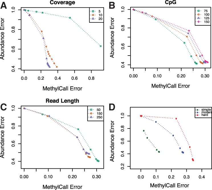
Average abundance error versus average methylation call error in different setting of simulation and various thresholds in moderate complexity of patterns. Points correspond to increasing threshold on methylation error between matched patterns. Panels show the effect of different (A) coverage, (B) number of CpG sites and (C) short read length on error. (D) Average abundance error versus average methylation call error in different simulated pattern complexity with fixed coverage, number of CpG and short read length

We observed that abundance error decreases and methylation call error increases as read length and coverage increases. Increasing coverage and read length help to decrease the problem complexity and have a more accurate reconstructed pattern. In particular, we observed that while doubling coverage from 5× to 10× significantly decreases error, doubling coverage from 10× to 20× has much less pronounced effect. Increasing the number of CpGs increases the complexity of the problem and both average abundance and average methylation call error increase. In this Figure 3D, CpG, read length and coverage are fixed, while pattern complexity is varied. Methylation call error and average abundance error increase as the complexity of patterns increases.

Supplementary Figure 1 shows the minimum cost network flow error metric for our three simulation settings as a function of coverage, number of CpGs and read length. By increasing coverage and read length, as we expect, the complexity of reconstruction decreases and the error decreases consequently with error decreasing sharply from 5× to 10× coverage, with slower decrease after that. Because we are reading CpG positions from a real data set, increasing the number of CpG sites are expanding the genomic region but the density of CpG sites remains almost the same. Hence, we see a slight increase in the error.

Our algorithm is less dependent on the number of CpGs. The performance of our algorithm slightly decreases by increasing number of CpGs and that is mainly because of the extension in the length of reconstructed region. Coverage has more significant effect on the performance of our algorithm. We see more errors in low coverage regions. Also our algorithm performs better if we could have longer sequencing reads and less ambiguity between cell-specific patterns.

We also evaluate sensitivity of our algorithm to error in sequencing CpG methylation status. Figure 4 shows that the minimum cost flow error increases by increasing the probability of noise. Note that when the noise level is 50, i.e. $p(error)=0.5$ in sequencing, then the short reads are random, and thus the output will be random, i.e. the minimum cost flow error is around 0.5. The regularization parameter λ indirectly controls the number of estimated patterns. As can be seen in Figure 4, the methylFlow algorithm is not sensitive to regularization parameter in a wide range of λ. In particular, methylFlow achieves consistently good performance with λ varying from 0 to 100 for different types of simulated data. This is an interesting property because we do not need to tune the regularization parameter precisely in the real data sets.

Fig. 4.

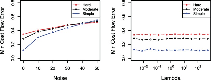
(Left) Sensitivity to the noise level in the input. Minimum cost flow error for various noise levels, probability error in sequencing, of the input data. (Right) Sensitivity to regularization parameter λ. Minimum cost flow error for various values of the regularization parameter

4.2 Single-cell sequencing data

We also evaluated our algorithm using a single-cell bisulfite sequencing (scBS-seq) dataset (Smallwood et al., 2014). Smallwood et al. performed scBS-Seq on mouse embryonic stem cells (ESCs) cultured either in 2i (2i ESCs) or serum (serum ESCs) conditions to determine whether scBS-Seq can reveal DNAm heterogeneity at the single-cell level. To evaluate the performance of our algorithm, we ran our algorithm separately on 2i and serum single-cell datasets that were aligned to GRCm38 mouse genome using Bismark in single-end mode. We observed that our algorithm reconstructed a single pattern for 93% of the regions covered and obtained two patterns for 6% of covered regions. We also ran methylFlow on a mixture of 2i and Serum samples. For 79% of regions, methylFlow recovered exactly the same number of patterns as expected from the mixture. For 17% of the regions, methylFlow recovered one fewer pattern than expected from the mixture. This result suggests that methylFlow is capable of identifying long-range methylation patterns in an epigenetically heterogeneous cell population. Unfortunately, coverage for single-cell sequencing data is too low to reliably estimate our algorithm’s performance in estimating the abundance of patterns in a heterogeneous cell population.

4.3 Ultra-high coverage-targeted sequencing

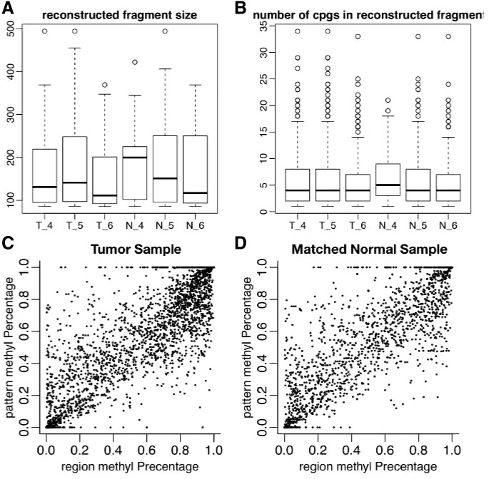
We applied our method to data from a targeted bisulfite sequencing experiment on three colon tumors and matched normal tissue (Hansen et al., 2011). Read lengths in this dataset are either 73 or 80 bp, and we used the provided read alignments with a post-processing script (available on request) to resolve strand-aware methylation status as reported by the alignment tool before constructing the read overlap graph. We were able to reconstruct cell-specific methylation patterns with median length 110–200 bp (Fig. 5. Patterns longer than 350 bp were reconstructed in each sample).

Fig. 5.

Pattern estimation in targeted bisulfite sequencing of three colon tumors and matched normal tissue in chromosome 13. (A) Length distributions of reconstructed cell-specific methylation patterns. (B) Distributions of the number of CpGs per reconstructed cell-specific methylation patterns. (C and D) CpG methylation percentage estimated from reconstructed cell-specific methylation patterns (pattern methyl Percentage) versus observed CpG methylation percentage (region methyl Percentage) for a single tumor sample and matched normal

Because the true cell-type methylation patterns are not known, the error metrics presented in Section 3.2 are not applicable. In real datasets, we instead report performance by comparing marginal methylation percentage of estimated patterns at CpG level to those estimated from short reads directly. Because we are not using this information in reconstructing patterns, similar beta value (marginal methylation percentage) could evaluate the performance of our method. Figure 5, panels C and D, shows the marginal methylation percentage from estimated patterns are highly correlated with marginal methylation estimates from short reads (correlation 0.89).

As illustration of the type of inference provided by our method, we show in Figure 6 the patterns estimated for a differentially methylated region. We obtained the most differentially methylated region in chromosome 13 using bumphunter software (Jaffe et al., 2012). The Figure depicts the estimated patterns in every sample along with their abundances in this hyper-methylated region. We observed that populations in tumor are more heterogenous than in normal (which itself is heterogenous to a small degree), and that dominant patterns in the normal population are present in the tumor population.

Fig. 6.

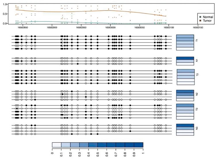
Differentially methylated region between colon tumors and matched normal pairs with corresponding patterns and their abundances across different samples. The top panel shows the marginal methylation percentage and the average curve of marginal methylation percentage as estimated by bumphunter. The bottom panel depicts the methylation patterns of samples. Blue bars represent the abundance of corresponding patterns. The abundances are normalized by sum of the abundances of all patterns in selected region

4.4 Whole genome sequencing

We also applied our method to a whole genome bisulfite sequencing (WGBS) data on mouse wild-type activated B cells and mouse CLP and KSL cells (Kieffer-Kwon et al., 2013) aligned using bismark_v0.11.1. The length of short reads is 50 bp, and all analyses were done relative to the mm10/GRCm38 assembly of the mouse genome. We were able to reconstruct cell-specific methylation patterns with median length 200–750 bp (Supplementary Fig. S2). Patterns longer than 750 bp were reconstructed in each sample.

Again, we report the performance of our method using the marginal methylation percentage of estimated patterns at CpGs to those obtained from short reads directly. Supplementary Figure 2, panels C and D, shows the marginal methylation estimates from patterns to those obtained from short reads (correlation 0.92 and 0.91).

5 Discussion and Conclusion

We have presented an algorithmic method to reconstruct cell-specific methylation patterns using overlap and coverage of sequencing reads of bisulfite-treated DNA. Our method allows researchers to probe intra-cellular epigenomic heterogeneity from a standard sequencing experiment of pooled cells. This work opens new avenues in the analysis of epigenomes as statistical extensions to our work here can start addressing questions of differential presence of cell-specific methylation patterns across phenotypes of interest, and begin to understand specific changes in the epigenomic complexity of cell communities.

Some cell-devoncolution methodologies like methylPurify (Zheng et al., 2014) use regions with bisulfite reads showing discordant methylation levels to infer tumor purity from tumor samples alone. They do not assume any genomic variation information or prior knowledge from other datasets. Some restrictions in their method is that they infer the fraction of normal cells within tumor samples by assuming that there are only two component of normal and tumor cells. They also detect differentially methylated regions from tumor and normal cell lines, under assumption of homogeneous tumor and normal cell lines. Because they only consider CpG sites, they expect to see consistent methylation level within short intervals (300 bp). Houseman et al. (2012) also present a statistical method to infer the distribution of different cells in a subpopulation and similarly, methylMix (Gevaert, 2015) developed a computational algorithm to identify differentially methylated genes that are also predictive of transcription. The two latter methods used the Illumina Infinium HumanMethylation 27k or 450k BeadChip.

Our simulation study shows that our methodology is sensitive, as other similar methods for sequencing data, to sequencing depth. Figure 3 indicates that that our approach works well at depths of ≥10×. Our software outputs total coverage per connected component in the region graph. In practice, regions that have <10× average coverage should be removed for downstream analysis.

While we have not applied our method to Reduced Representation Bisulfite Sequencing (RRBS) data (Meissner et al., 2005), it should directly apply as presented in this manuscript, under the same caveats regarding coverage discussed above. RRBS is designed for high-density regions, and usually tends to yield higher coverage than WGBS, which makes it suitable for our methodology. Our method requires single-fragment methylation calls as input as provided by sequencing assays, which makes it unsuitable for array-based assays, tiling (Irizarry et al., 2008) or based on Bisulfite conversion as signal in this case depends on the number of methylated and unmethylated fragments in a pool of cells (Bibikova et al., 2011). While we believe that our normalization method somewhat alleviates coverage biases stemming from sequence or amplification effects, a normalization model that incorporates relevant technical covariates could significantly improve any instability in our estimation method stemming from coverage biases.

As presented here, our method only performs reconstruction of patterns for single samples (e.g. a single tumor sample). A consideration for future work is to establish an algorithm that jointly estimates cell-specific methylation patterns across samples. However, our graph matching procedures described in Section 3.2 can be used to associate estimated patterns across individual samples in subsequent analyses.

References

- Bernard E. et al. (2014) Efficient RNA isoform identification and quantification from RNA-Seq data with network flows. Bioinformatics (Oxford, England), 30, 2447–2455. [DOI] [PMC free article] [PubMed] [Google Scholar]
- Bibikova M. et al. (2011) High density DNA methylation array with single CpG site resolution. Genomics, 98, 288–295. [DOI] [PubMed] [Google Scholar]
- Dezső B. et al. (2011) Lemon–an open source c ++ graph template library. Electron. Notes Theor. Comput. Sci., 264, 23–45. [Google Scholar]
- Eriksson N. et al. (2008) Viral population estimation using pyrosequencing. PLOS Comput. Biol., 4, e1000074.. [DOI] [PMC free article] [PubMed] [Google Scholar]
- Gevaert O. (2015) Methylmix: an R package for identifying DNA methylation-driven genes. Bioinformatics, 31, 1839–1841. [DOI] [PMC free article] [PubMed] [Google Scholar]
- Hansen K.D. et al. (2011) Increased methylation variation in epigenetic domains across cancer types. Nat. Genet., 43, 768–775. [DOI] [PMC free article] [PubMed] [Google Scholar]
- Hansen K.D. et al. (2012) BSmooth: from whole genome bisulfite sequencing reads to differentially methylated regions. Genome Biol., 13, R83.. [DOI] [PMC free article] [PubMed] [Google Scholar]
- Holliday R., Pugh J.E. (1975) DNA modification mechanisms and gene activity during development. Science (New York, NY), 187, 226–232. [PubMed] [Google Scholar]
- Houseman E.A. et al. (2012) DNA methylation arrays as surrogate measures of cell mixture distribution. BMC Bioinformatics, 13, 86.. [DOI] [PMC free article] [PubMed] [Google Scholar]
- Irizarry R.A. et al. (2008) Comprehensive high-throughput arrays for relative methylation (CHARM). Genome Res., 18, 780–790. [DOI] [PMC free article] [PubMed] [Google Scholar]
- Jaffe A.E. et al. (2012) Bump hunting to identify differentially methylated regions in epigenetic epidemiology studies. Int. J. Epidemiol., 41, 200–209. [DOI] [PMC free article] [PubMed] [Google Scholar]
- Kieffer-Kwon K.R. et al. (2013) Interactome maps of mouse gene regulatory domains reveal basic principles of transcriptional regulation. Cell, 155, 1507–1520. [DOI] [PMC free article] [PubMed] [Google Scholar]
- Krueger F., Andrews S.R. (2011) Bismark: a flexible aligner and methylation caller for Bisulfite-Seq applications. Bioinformatics (Oxford, England), 27, 1571–1572. [DOI] [PMC free article] [PubMed] [Google Scholar]
- Landan G. et al. (2012) Epigenetic polymorphism and the stochastic formation of differentially methylated regions in normal and cancerous tissues. Nat. Genet., 44, 1207–1214. [DOI] [PubMed] [Google Scholar]
- Li W. et al. (2011) Isolasso: a lasso regression approach to RNA-Seq based transcriptome assembly. J. Comput. Biol., 18, 1693–1707. [DOI] [PMC free article] [PubMed] [Google Scholar]
- Lister R. et al. (2009) Human DNA methylomes at base resolution show widespread epigenomic differences. Nature, 462, 315–322. [DOI] [PMC free article] [PubMed] [Google Scholar]
- Luenberger D.G. (1973) Introduction to Linear and Nonlinear Programming, Vol. 28 Addison-Wesley, Reading, MA, USA. [Google Scholar]
- Makhorin A. (2008) GNU Linear Programming Kit, Version 4.47. http://www.gnu.org/software/glpk/glpk.html.
- Meissner A. et al. (2005) Reduced representation bisulfite sequencing for comparative high-resolution DNA methylation analysis. Nucleic Acids Res., 33, 5868–5877. [DOI] [PMC free article] [PubMed] [Google Scholar]
- Smallwood S.A. et al. (2014) Single-cell genome-wide bisulfite sequencing for assessing epigenetic heterogeneity. Nat. Methods, 11, 817–820. [DOI] [PMC free article] [PubMed] [Google Scholar]
- Timp W. et al. (2014) Large hypomethylated blocks as a universal defining epigenetic alteration in human solid tumors. Genome Med., 6, 61.. [DOI] [PMC free article] [PubMed] [Google Scholar]
- Zheng X. et al. (2014) Methylpurify: tumor purity deconvolution and differential methylation detection from single tumor DNA methylomes. Genome Biol., 15, 419. [DOI] [PMC free article] [PubMed] [Google Scholar]
Associated Data
This section collects any data citations, data availability statements, or supplementary materials included in this article.