What time is it? Deep learning approaches for circadian rhythms

Abstract

Motivation: Circadian rhythms date back to the origins of life, are found in virtually every species and every cell, and play fundamental roles in functions ranging from metabolism to cognition. Modern high-throughput technologies allow the measurement of concentrations of transcripts, metabolites and other species along the circadian cycle creating novel computational challenges and opportunities, including the problems of inferring whether a given species oscillate in circadian fashion or not, and inferring the time at which a set of measurements was taken.

Results: We first curate several large synthetic and biological time series datasets containing labels for both periodic and aperiodic signals. We then use deep learning methods to develop and train BIO_CYCLE, a system to robustly estimate which signals are periodic in high-throughput circadian experiments, producing estimates of amplitudes, periods, phases, as well as several statistical significance measures. Using the curated data, BIO_CYCLE is compared to other approaches and shown to achieve state-of-the-art performance across multiple metrics. We then use deep learning methods to develop and train BIO_CLOCK to robustly estimate the time at which a particular single-time-point transcriptomic experiment was carried. In most cases, BIO_CLOCK can reliably predict time, within approximately 1 h, using the expression levels of only a small number of core clock genes. BIO_CLOCK is shown to work reasonably well across tissue types, and often with only small degradation across conditions. BIO_CLOCK is used to annotate most mouse experiments found in the GEO database with an inferred time stamp.

Availability and Implementation: All data and software are publicly available on the CircadiOmics web portal: circadiomics.igb.uci.edu/.

Contacts: fagostin@uci.edu or pfbaldi@uci.edu

Supplementary information: Supplementary data are available at Bioinformatics online.

1 Introduction

The importance of circadian rhythms cannot be overstated: circadian oscillation have been observed in animals, plants, fungi and cyanobacteria and date back to the very origins of life on Earth. Indeed, some of the most ancient forms of life, such as cyanobacteria, use photosynthesis as their energy source and thus are highly circadian almost by definition. These oscillations play a fundamental role in coordinating the homeostasis and behavior of biological systems, from the metabolic (Eckel-Mahan and Sassone-Corsi, 2009; Froy, 2011; Takahashi et al., 2008; Yoo et al., 2004) to the cognitive levels (Eckel-Mahan et al., 2008; Gerstner et al., 2009). Disruption of circadian rhythms has been directly linked to health problems (Knutsson, 2003; Lamia et al., 2008; Takahashi et al., 2008) ranging from cancer, to insulin resistance, to diabetes, to obesity and to premature ageing (Antunes et al., 2010; Froy, 2010, 2011; Karlsson et al., 2001; Kohsaka et al., 2007; Kondratov et al., 2006; Sharifian et al., 2005; Shi et al., 2013; Turek et al., 2005). At their most fundamental level, these oscillations are molecular in nature, whereby the concentrations of specific molecular species such as transcripts, metabolites and proteins oscillate in the cell with a 24 h periodicity. Modern high-throughput technologies allow large-scale measurements of these concentrations along the circadian cycle thus creating new datasets and new computational challenges and opportunities. To mine these new datasets, here we develop and apply machine learning methods to address two questions: (i) which molecular species are periodic? and (ii) what time or phase is associated with high-throughput transcriptomic measurements made at a single timepoint?

At the molecular level, circadian rhythms are in part driven by a genetically encoded, highly conserved, core clock found in nearly every cell based on negative transcription/translation feedback loops, whereby transcription factors drive the expression of their own negative regulators (Partch et al., 2014; Schibler and Sassone-Corsi, 2002), and involving only a dozen genes (Partch et al., 2014; Yan et al., 2008). In the mammalian core clock (Fig. 1), two bHLH transcription factors, CLOCK and BMAL1 heterodimerize and bind to conserved E-box sequences in target gene promoters, thus driving the rhythmic expression of mammalian Period (Per1, Per2 and Per3) and Cryptochrome (Cry1 and Cry2) genes (Stratmann and Schibler, 2006). PER and CRY proteins form a complex that inhibits subsequent CLOCK:BMAL1-mediated gene expression (Brown et al., 2012; Dibner et al., 2010; Partch et al., 2014). The master core clock located in the suprachiasmatic nucleus (SCN) (Moore and Eichler, 1972; Ralph et al., 1990) of the hypothalamus interacts with the peripheral core clocks throughout the body (Takahashi et al., 2008; Yoo et al., 2004).

Fig. 1.

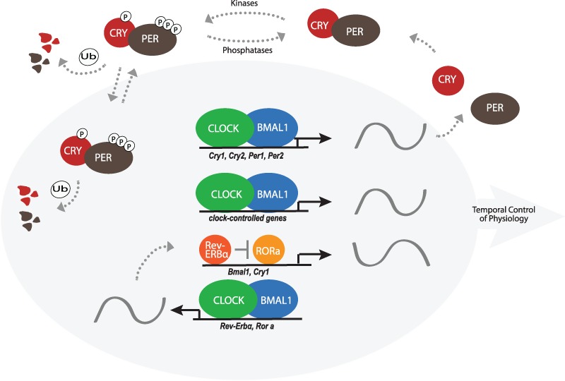
Core clock genes and proteins and the corresponding transcription/translation negative feedback loop

In contrast to the small size of the core clock, high-throughput transcriptomic (DNA microarrays, RNA-seq) or metabolomic (mass spectrometry) experiments (Andrews et al., 2010; Eckel-Mahan et al., 2012, 2013; Hughes et al., 2009; Masri et al., 2014b; Miller et al., 2007; Panda et al., 2002; P.Tognini et al., in preparation), have revealed that a much larger fraction, typically on the order of 10%, of all transcripts or metabolites in the cell are oscillating in a circadian manner. Furthermore, the oscillating transcripts and metabolites differ by cell, tissue type, or condition (Panda et al., 2002; Storch et al., 2002; Yan et al., 2008). Genetic, epigenetic and environmental perturbations—such as a change in diet—can lead to cellular reprogramming and profoundly influence which species are oscillating in a given cell or tissue (Bellet et al., 2013; Dyar et al., 2014; Eckel-Mahan et al., 2012, 2013; Masri et al., 2013, 2014a). When results are aggregated across tissues and conditions, a very large fraction, often exceeding 50% and possibly approaching 100%, of all transcripts is capable of circadian oscillations under at least one set of conditions, as shown in plants (Covington et al., 2008; Harmer et al., 2000), cyanobacteria and algae (Monnier et al., 2010; Vijayan et al., 2009) and mouse (Patel et al., 2015; Zhang et al., 2014).

In a typical circadian experiment, high-throughput omic measurements are taken at multiple timepoints along the circadian cycle under both control and treated conditions. Thus the first fundamental problem that arises in the analysis of such data is the problem of detecting periodicity, in particular circadian periodicity, in these time series. The problem of detecting periodic patterns in time series is of course not new. However, in the cases considered here the problem is particularly challenging for several reasons, including: (i) the sparsity of the measurements (the experiments are costly and thus data may be collected for instance only every 4 h); (ii) the noise in the measurements and the well known biological variability; (iii) the related issue of small sample sizes (e.g. n = 3); (iv) the issue of missing data; (v) the issue of uneven sampling in time; and (vi) the large number of measurements (e.g. 20 000 transcripts) and the associated multiple-hypothesis testing problem. Here we develop and apply deep learning methods for robustly assessing periodicity in high-throughput circadian experiments, and systematically compare the deep learning approach to the previous, non-machine learning, approaches (Glynn et al., 2006; Hughes et al., 2010; Yang and Su, 2010). While this is useful for circadian experiments, the vast majority of all high-throughput expression experiments have been carried, and continue to be carried, at single timepoints. This can be problematic for many applications, including applications to precision medicine, precisely because circadian variations are ignored creating possible confounding factors. This raises the second problem of developing methods that can robustly infer the approximate time at which a single-time high-throughput expression measurement was taken. Such methods could be used to retrospectively infer a time stamp for any expression dataset, in particular to improve the annotations of all the datasets contained in large gene expression repositories, such as the Gene Expression Omnibus (GEO) (Edgar et al., 2002), and improve the quality of all the downstream inferences that can be made from this wealth of data. There may be other applications of such a method, for instance in forensic sciences, to help infer a time of death. In any case, to address the second problem we also develop and apply deep learning methods to robustly infer time or phase for single-time high-throughput gene expression measurements.

2 Datasets

2.1 Periodicity inference from time series measurements

To train and evaluate the deep learning methods, we curate BioCycle, the largest dataset including both synthetic and real-world biological time series, and both periodic and aperiodic signals. While the main goal here is to create methods to analyze real-world biological data, relying only on biological data to determine the effectiveness of a method is not sufficient because there are not many biological samples which have been definitively labeled as being periodic or aperiodic. Even when one can be confident that a signal is periodic, it can be difficult to determine the true period, phase and amplitude of that signal. Therefore, we rely also on synthetic data to provide us with signals that we can say are definitely periodic or aperiodic, and whose attributes—such as period, amplitude, and phase—can be controlled and are known. Furthermore, previous approaches were developed using synthetic data and thus the same synthetic data must be used to make fair comparisons.

2.1.1 Synthetic data

We first curate a comprehensive synthetic dataset BioCycle_Synth, which includes all previously defined synthetic signals found in JTK_Cycle (Hughes et al., 2010) and ARSER (Yang and Su, 2010), but also contains new signals. BioCycle_Synth is in turn a collection of two different types of datasets: a dataset in which signals are constructed using mathematical formulas (BioCycle_Form), and a dataset in which signals are generated from a Gaussian process (Rasmussen, 2004) (BioCycle_Gauss). In previous work, synthetic data was generated with carefully constructed formulas to try to mimic periodic signals found in real-world data (see below). While this gives one a lot of control over the data, it can create signals that are too contrived and therefore not representative of real-world biological variations. In addition, the noise added at each timepoint is independent of the other timepoints, which may not be the case in real-world data. The BioCycle_Gauss dataset uses Gaussian processes to generate the data and address these problems.

The datasets used in JTK_Cycle contain the following types of formulas or signals: cosine, cosine with outlier timepoints and white noise. The ARSER dataset contains cosine, damped cosine with an exponential trend, white noise and an auto-regressive process of order 1 (AR(1)). In addition to all the aforementioned signals, BioCycle_Form contains also 9 additional kinds of signals: combined cosines (cosine2), cosine peaked, square wave, triangle wave, cosine with a linear trend, cosine with an exponential trend, cosine multiplied by an exponential, flat and linear signals (many of which can be found in Deckard et al., 2013). Figure 2 shows an example of each type of signal found in the BioCycle_Form dataset. For clarity, the periodic signals are shown without noise. Signals in the BioCycle_Form dataset have an additional random offset chosen uniformly between −200 and 200, random amplitudes chosen uniformly between 1 and 100, signal to noise ratios (SNRs) of 1–5, random phases chosen uniformly between 0 and $2\pi$, and periods between 20 and 28. [Data for the second (12 h) and third (8 h) harmonics, which are found in biological data, are also generated (Supplementary Information)]. At each timepoint sample, zero mean Gaussian noise is added with the proper SNR variance.

Fig. 2.

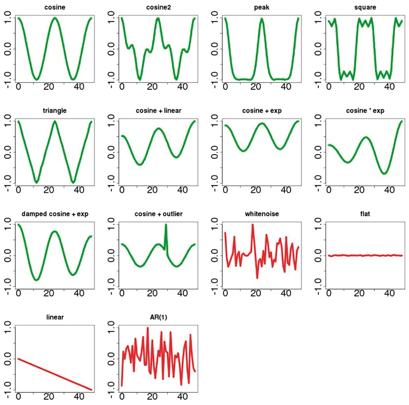
Samples of synthetic signals in the BioCycle_Form dataset. Signals in green are periodic; signals in red are aperiodic

The BioCycle_Gauss dataset is obtained from a Gaussian process. The value of the covariance matrix corresponding to the timepoints x and $x\prime$ is determined by a kernel function $k(x,x\prime )$. Equation 1 is the kernel function used to generate the periodic signals, and Equation 2 is the kernel function used to generate the aperiodic signals in BioCycle_Gauss .

$$k_p(x,x\prime )=\text{exp}\left(\frac{-{\text{sin}}^2(|\pi \frac{1}{p}(x-x\prime )|)}{2l^2}\right)+{\sigma }^2\delta (x,x\prime )+\beta xx\prime$$ (1)

$$k_a(x,x\prime )=\text{exp}\left(\frac{-{(x-x\prime )}^2}{2l^2}\right)+{\sigma }^2\delta (x,x\prime )$$ (2)

The parameter l controls how strong the covariance is between two different timepoints, σ controls how noisy the synthetic data is, and β can add a non-stationary, linear, trend to the signals (Duvenaud, 2014). The parameter p in equation 1 is the period of the signal. To generate the data in BioCycle_Gauss, the values of l, σ, β, p, as well as the offset and the scale are varied, in a way similar to the data in BioCycle_Form . Examples of signals from the BioCycle_Gauss dataset are given in Figure 3.

Fig. 3.

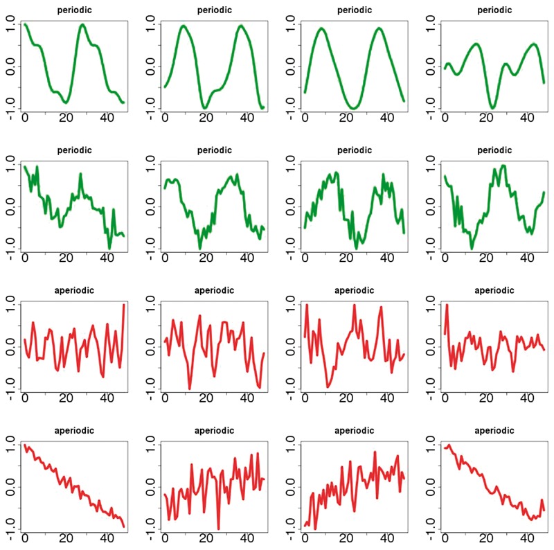
Samples of synthetic signals in the BioCycle_Gauss dataset. Signals in green are periodic; signals in red are aperiodic

JTK_Cycle analyzes synthetic signals sampled over 48 h with a sampling frequency of 1 and 4 h. ARSER analyzes synthetic signals sampled over 44 h with a sampling frequency of 4 h. BioCycle analyzes synthetic signals sampled over 24 and 48 h. Signals sampled over 24 h have a sampling frequency of 4, 6 and an uneven sampling at timepoints 0, 5, 9, 14, 19 and 24. Signals sampled over 48 h have sampling frequencies of 4, 8 and an uneven sampling at timepoints 0, 4, 8, 13, 20, 24, 30, 36, 43. The sampling frequencies in these datasets are intentionally sparse to mimic the sparse temporal sampling of real-world high-throughput data. The number of synthetic signals at each sampling frequency is 1024 for JTK_Cycle, 20 000 for ARSER and 40 000 for BioCycle_Synth . Finally, each signal in BioCycle_Synth has three replicates, obtained by adding random Gaussian noise to the signal, to mimic typical biological experiments.

2.1.2 Biological data

The performance of any circadian rhythm detection method requires extensive validation on biological datasets. In previous work, due to the aforementioned difficulty of not having ground truth labels, the biological signals detected as being periodic had to be inspected by hand, or loosely assessed by comparison to other methods (Straume, 2004). In addition to the scaling problems associated with manual inspection, this approach did not allow the computation of precise classification metrics (Baldi et al., 2000), such as the AUC—the Area Under the Receive Operating Characteristic (ROC) Curve. The repository of circadian data hosted on CircadiOmics (Patel et al., 2012) includes over 30 high-throughput circadian transcriptomic studies, as well as several circadian high-throughput metabolomic studies, that provide extensive coverage of different tissues and experimental conditions. From the CircadiOmics data, a high-quality biological dataset BioCycle_Real is created with periodic/aperiodic labels.

To curate BioCycle_Real, we start from 36 circadian microarray or RNA-seq transcriptome datasets, 32 of which are currently publicly available from the CircadiOmics web portal (28 of these are also available from CircaDB (Pizarro et al., 2012)). Five datasets are from ongoing studies and will be added to CircadiOmics upon completion. All included datasets correspond to experiments carried out in mice, with the exception of one dataset corresponding to measurements taken in Arabidopsis Thaliana. BioCycle_Real comprises experiments carried over a: 24-h period with a 4 h sampling rate; 48-h period with a 2 h sampling rate; and 48-h period with a 1 h sampling rate.

To extract from this set a high-quality subset of periodic time series, we focus on the time series associated with the core clock genes (Fig. 1) in the control experiments. These gene include Clock, Per1, Per2, Per3, Cyr1, Cry2, Nr1d1, Nr1d2, Bhlhe40, Bhlhe41, Dbp, Npas2 and Tel (Harmer et al., 2001) for mouse, and the corresponding orthologs in Arabidopsis (Harmer et al., 2000). Arabdiposis orthologs were obtained from Affymetrix NetAffx probesets and annotations (Liu et al., 2003). These core gene time series were further inspected manually to finally yield a set of 739 high-quality periodic signals. To extract a high-quality biological aperiodic dataset, we start from the same body of data. To identify transcripts unlikely to be periodic, we select the transcripts classified as aperiodic consistently by all three programs JTK_Cycle, ARSER and Lomb-Scargle with an associated P-value of 0.95. After further manual inspection, this yields a set of 18 094 aperiodic signals. Examples of signals taken at random from the BioCycle_Real are shown in Figure 4.

Fig. 4.

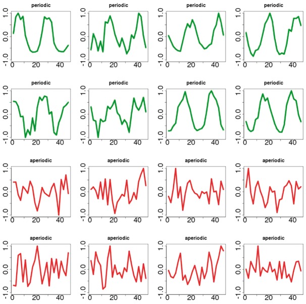
Samples of biological time series in the BioCycle_Real dataset. Signals in green are periodic; signals in red are aperiodic. [Note the signals are spline-smoothed.]

2.2 Time inference from single timepoint measurements

To estimate the time associated with a transcriptomic experiment conducted at a single timepoint, we curate the BioClock dataset starting from the same data in CircadiOmics, focusing on mouse data only for which we have enough training data. While in principle inference of the time can be done using the level of expression of all the genes, exploratory feature selection and data reduction experiments (not shown) show that in most cases it is sufficient to focus on the set of core clock genes, or even a subset (see Section 4). Thus the reduced BioClock dataset contains microarray and RNA-Seq single time measurements for each gene transcript in the core clock with the associated timepoint. The BioClock dataset is organized by tissue and condition. Tissues include liver, kidney, heart, colon, glands (pituitary, adrenal), skeletal muscle, bone, white fat and brown fat. Brain specific tissues include SCN (Suprachiasmatic nucleus), hippocampus, hypothalamus and cerebellum. There are also several cell-specific datasets including mouse fibroblasts and macrophages. All the datasets in BioClock contain both control and treatment conditions. There is great variability among the treatment conditions (e.g. Eckel-Mahan et al., 2013; Masri et al., 2014a), varying from gene knock out and knock down (SIRT1 and SIRT6), to changes in diet (high fat, ketogenic), to diseases (epilepsy). It is important to be able to assess the ability of a system to predict time across tissues and conditions.

3 Methods

We experimented with several machine learning approaches for the two main problems considered here. In general, the best results were obtained using neural networks. This is perhaps not too surprising since it is well known that neural networks have universal approximation properties and deep learning has led to state-of-the art performance, not only in several areas of engineering (e.g. computer vision, speech recognition, natural language processing, robotics) (Hannun et al., 2014; Lenz et al., 2015; Szegedy et al., 2014), but also in the natural sciences (Baldi et al., 2014; Di Lena et al., 2012; Lusci et al., 2013; Quang et al., 2015). Thus here we focus exclusively on deep learning approaches to build two systems, BIO_CYCLE and BIO_CLOCK, to address the two main problems. However, we add comparisons to k-nearest neighbors and Gaussian processes in the Supplementary Information.

3.1 Periodicity inference from time series measurements

3.1.1 Classifying between periodic and aperiodic signals

To classify signals as periodic or aperiodic, we train deep neural networks (DNNs) using standard gradient descent with momentum (Rumelhart et al., 1988; Sutskever et al., 2013). We train separate networks for data sampled over 24 and 48 h. The input to these networks are the expression time-series levels of the corresponding gene (or metabolite). The output is computed by a single logistic unit trained to be 1 when the signal is periodic and 0 otherwise, with relative entropy error function. We experimented with many hyperparameters and learning schedules. In the results reported, the learning rate starts at 0.01, and decays exponentially according to $\frac{0.1}{{1.000087}^t}$, where t is the iteration number. The training set consists of 1 million examples, a size sufficient to avoid overfitting. The DNN uses a mini-batch size of 100 and is trained for 50 000 iterations. Use of dropout (Baldi and Sadowski, 2014; Srivastava et al., 2014), or other forms of regularization, leads to no tangible improvements. The best performing DNN found (Fig. 5(a)) has 3 hidden layers of size 100. We are able to obtain very good results by training BIO_CYCLE on synthetic data alone and report test results obtained on BioCycle_Form, BioCycle_Gauss and BioCycle_Real .

Fig. 5.

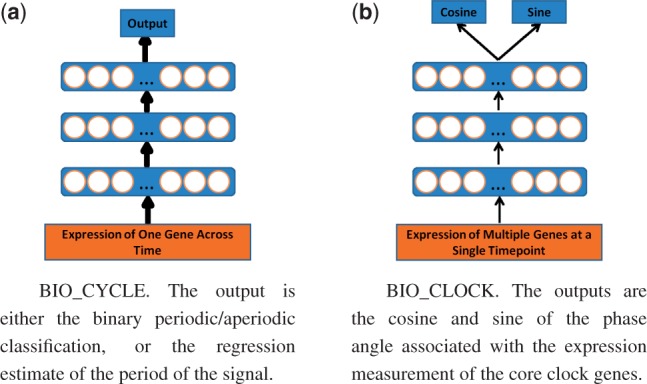
Visualizations of the deep neural networks (DNNs)

3.1.2 Estimating the period

In a way similar to how we train DNNs to classify between periodic and aperiodic signals, we can also train DNNs to estimate the period of a signal classified as periodic. During training, only periodic time series are used as input to train these regression DNNs. The output of the DNNs are implemented using a linear unit and produce an estimated value for the period. The error function is the squared error between the output of the network and the true period of the signal, which is known in advance with synthetic data. Except for the difference in the output unit, we use the same DNNs architectures and hyperparameters as for the previous classification problem.

3.1.3 Estimating the phase and the lag

After the period p, we estimate the phase $\varphi$ of a signal s by finding the value $\varphi$ that maximizes the following expression: $\sum _{t\in T}\text{cos}(\frac{2\pi t}{p}+\varphi )s[t]$, where T is the set of all timepoints. Given $\varphi$, the lag (i.e. at what time the periodic pattern starts) is given by $\frac{\varphi p}{2\pi }$.

3.1.4 Estimating the amplitude

After the phase $\varphi$, we estimate the amplitude α by first removing any linear trend and then comparing the variance of the signal to the variance of a cosine signal with parameters $\varphi$, p and amplitude 1. The formula is shown in Equation 3, where ${\mu }_s=\frac{1}{\left|T\right|}\sum _{t\in T}s[t]$ and ${\mu }_c=\frac{1}{\left|T\right|}\sum _{t\in T}\text{cos}(\frac{2\pi t}{p}+\varphi )$

$$\alpha =\sqrt{\frac{\frac{1}{\left|T\right|}{\displaystyle \sum _{t\in T}{(s[t]-{\mu }_s)}^2}}{\frac{1}{\left|T\right|}{\displaystyle \sum _{t\in T}(\text{cos}(}\frac{2\pi t}{p}+\varphi )-{\mu }_c{)}^2}}$$ (3)

We cannot claim this approach is new, however, we have not seen it in previous literature. An alternative is to measure the amplitude on the smoothed time series.

3.1.5 Calculating P-values and q-values

To calculate P-values, the distribution of the null hypothesis must first be obtained. To do this, N aperiodic signals are generated from one of the two BioCycle_Synth datasets. Then we calculate the N output values V(i) ($i=1,\dots ,N$) of the DNN on these aperiodic signals. The P-value for a new signal s with output value V is now $\frac{1}{N}{\displaystyle {\sum }_{i=1}^N}\mathrm{1}(V>V(i))$, where 1 is the indicator function. This equation provides an empirical frequency estimate for the probability of obtaining an output of size V or greater, assuming that the signal s comes from the null distribution (the distribution of aperiodic signals). Therefore, the smaller the P-value, the more likely it is that s is periodic. The q-values are obtained through the Benjamini and Hochberg procedure (Benjamini and Hochberg, 1995). We also compute a posterior probability of periodic expression (PPPE) using the method described in Allison et al. (2002), which models the distribution of P-values as a mixture of beta distributions.

3.2 Time inference from single timepoint measurements

For this task, different machine learning methods were investigated, including simple linear regression, k-nearest neighbors, decision trees, shallow learning and deep learning, including unsupervised compressive autoencoders (Baldi, 2012) with two coupled phase (cosine/sine) units in the bottleneck layer (below and Supplementary Information). Supervised deep learning methods give the best results and are used in the final BIO_CLOCK system. The output of the DNNs is implemented using two coupled output units, representing the cosine and the sine of the phase angle (Fig. 5(b)). If the total weighted inputs into these two units are S₁ and S₂ respectively, then the values of the two outputs units are given by: $S_1/\sqrt{S_1^2+S_2^2}$ and $S_2/\sqrt{S_1^2+S_2^2}$. These are then automatically converted into a time (ZT). In order to better assess the effect of having data from different tissues, we experiment with both training specialized predictors trained on data originating from a single tissue, as well as predictors trained on data from all tissues. The final general-purpose predictor corresponds to a DNN trained on all the data. In each one of these experiments, we use 5-fold cross validation on the corresponding subset of the BioClock dataset, using architectures with 2 to 9 layers, and 100 to 600 units, to select the best network. A learning rate of 0.1 is typically used, with an exponential decay according to $\frac{0.1}{{1.002}^t}$. A visualization of the DNN is provided in Figure 5(b).

3.3 Data normalization

For both the periodicity and time inference problems, training and testing examples are normalized to have a mean of zero and a standard deviation of one.

3.4 Software and run time

Downloadable software is currently written in R and Python and is intended to be easy for biologists to use. While exploring different models both Pylearn2 (Goodfellow et al., 2013) and Caffe (Jia et al., 2014) were used. The DNNs typically take hours for training but, once trained, can process a real-world dataset (∼20 000 time series) in about one minute, both run times corresponding to a single CPU.

4 Results

In all the tables, the best results are shown in bold.

4.1 Periodic/aperiodic classification

For comparison, the methods ARSER (ARS), Lomb-Scargle (LS) and JTK_Cycle (JTK) are all evaluated along with the DNNs used by BIO_CYCLE, trained on the BioCycle_Form and BioCycle_Gauss datasets. In addition, we compare to MetaCycle (MC) (Wu et al., 2016). To identify periodic signals, ARSER uses autoregressive spectral estimation, Lomb-Scargle uses a periodogram, and JTK_Cycle uses the Jonckheere-Terpstra’s and the Kendall’s tau tests. MetaCycle combines ARSER, Lomb-Scargle and JTK_Cycle into one method.

To determine if the BIO_CYCLE results are significantly different from other methods, the testing set is randomly split into 10 equal-size, non-overlapping, subsets and the results from each subset are obtained. Then, a Student’s t-test is performed between the results of the best of the two DNNs and the best of the previously existing methods. Finally, the P-value from that test is obtained to assess if the result differences are statistically significant. Small P-values (such as 0.05 and below) indicate that there is a significant difference between the methods. The P-values from the t-tests are shown in the rightmost column in all the tables. The results focus on periodic signals with periods around 24 h, the most common case, however periods of 12 and 8 h, corresponding to the second and third harmonics, are analyzed in the Supplementary Information.

In the tables, the datasets BioCycle_Form, BioCycle_Gauss and BioCycle_Real are referred to as BC_F, BC_G and BC_R, respectively.

4.1.1 Synthetic data (BioCycle_Synth)

Results for the area under the receiver operating characteristic curve (AUC) for the task of classifying signals as periodic or aperiodic are shown in Table 1, and the ROC curves computed on BioCycle_Form are shown in Figure 6. The DNN_F label corresponds to the DNN that has been trained on the BioCycle_Form data, and the DNN_G label corresponds to the DNN that has been trained on the BioCycle_Gauss data. The ROC curves computed on BioCycle_Gauss are similar (not shown). The results from Table 1 show that the DNN method has better AUC than all the other published methods on the BioCycle_Form and BioCycle_Gauss datasets. Though the DNN does better when tested on data from the same distribution as it was trained on, it still outperforms all the other previous methods, regardless of which data it is trained on. A plot showing how the signal to noise ratio (SNR) affects performance is shown in Figure 7. This plot cannot be done for the BioCycle_Gauss dataset, since in this case the exact SNR is not known. The DNN outperforms all the other published methods at all SNRs.

Table 1.

AUC performance on synthetic data

	ARS	LS	JTK	MC	DNNF	DNNG	t-test
BCF (24_4)	0.85	0.86	0.87	0.87	0.92	0.91	0E+00
BCF (24_6)	0.72	0.81	0.76	0.81	0.85	0.84	0E+00
BCF (48_4)	0.94	0.95	0.95	0.95	0.97	0.96	3E-06
BCF (48_8)	0.83	0.86	0.78	0.86	0.89	0.89	1E-06
BCF (24_U)	0.80	0.84	0.85	0.84	0.89	0.88	0E+00
BCF (48_U)	0.89	0.92	0.83	0.92	0.94	0.93	0E+00
BCG (24_4)	0.85	0.89	0.89	0.89	0.92	0.94	0E+00
BCG (24_6)	0.73	0.85	0.78	0.85	0.88	0.89	1E-06
BCG (48_4)	0.96	0.95	0.95	0.96	0.97	0.97	5E-04
BCG (48_8)	0.90	0.91	0.80	0.92	0.93	0.93	2E-06
BCG (24_U)	0.84	0.89	0.88	0.89	0.91	0.92	0E+00
BCG (48_U)	0.93	0.94	0.85	0.94	0.95	0.96	2E-06
ARS (44_4)	0.99	0.98	0.97	0.99	0.99	0.99	0E+00
JTK (48_1)	1.00	1.00	1.00	1.00	1.00	1.00	2E-01
JTK (48_4)	0.96	0.97	0.98	0.98	0.98	0.97	1E+00

Fig. 6.

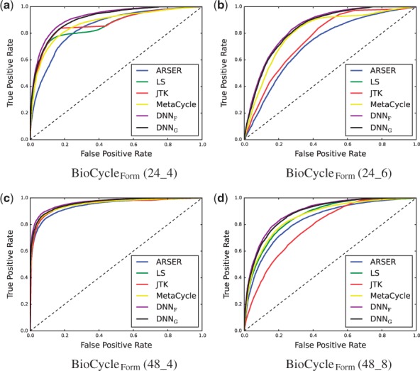
ROC Curves of different methods on the BioCycle_Form dataset

Fig. 7.

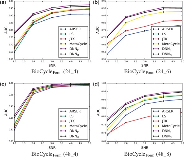
AUC at various signal-to-noise ratios (SNRs) on the BioCycle_Form dataset. The lower the SNR the noisier the signal is

4.1.2 Biological data (BioCycle_Real)

The performance on the biological dataset is shown in Table 2. Although the ARSER, LS and JTK_Cycle methods achieve good performance on the aperiodic data, as can be expected since they were used to label the aperiodic data, the DNN method remains very competitive, often outperforming at least one of the other published methods.

Table 2.

AUC performance on the biological dataset

	ARS	LS	JTK	MC	DNNF	DNNG	t-test
BCR (24_4)	0.97	0.97	0.89	0.97	0.97	0.97	7E-01
BCR (48_1)	0.96	0.94	0.91	0.98	0.98	0.97	5E-01
BCR (48_2)	0.98	0.97	0.95	0.96	0.94	0.95	3E-01

4.1.3 Evaluation of P-value cutoffs

To investigate if the p-values obtained by BIO_CYCLE are reasonable, the accuracy of the periodic/aperiodic classification at different p-value cutoffs is evaluated. In addition to a p-value, BIO_CYCLE produces a binary classification. If the output of the DNN is greater than 0.5 the signals is labeled as periodic, otherwise, it is labeled as aperiodic. The accuracy using this binary classification is also evaluated. Results are shown in Figure 8. The vertical dashed line corresponds to a common p-value cutoff of 0.05. However, a proper p-value does not guarantee that the best accuracy will be at the cutoff of 0.05. Results show that BIO_CYCLE has the highest potential accuracy. It also has the best accuracy at 0.05 for 2 out of the 4 plots. In addition, the binary classification of BIO_CYCLE is almost always better than the accuracy of all the other methods at any p-value cutoff. Histograms showing the p-values can be found in the Supplementary Information.

Fig. 8.

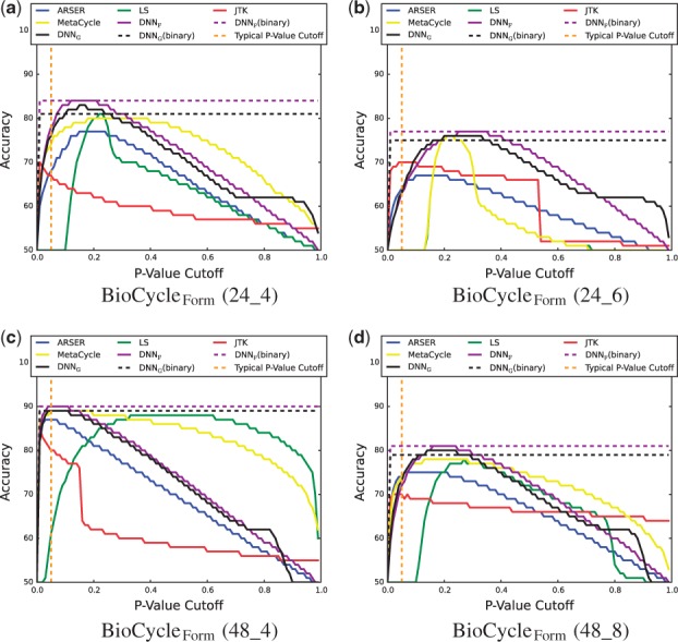
Accuracy of periodic/aperiodic classification at different p-value cutoffs on the BioCycle_Form dataset

4.2 Period, lag and amplitude estimation

The metric to determine how well each method estimates the period, lag and amplitude is given by the coefficient of determination R². The line y = x corresponds to perfect prediction. In this case, y is the estimated value given by the method and x is the true value. R² measures how well the line y = x fits the points that correspond to the true value versus the estimated value. Perfect prediction corresponds to y = x and corresponds to $R^2=1$. The results for estimating the period, lag and amplitude are shown in Tables 3–5, respectively. For the BioCycle_Gauss dataset we cannot control or know the exact lag or amplitude, so there are no results for BioCycle_Gauss in Tables 4 and 5. These tables tell a similar story as Table 1. The DNN outperforms the other methods in most of the categories. Even when the DNN is tested on data associated with a distribution that is different from the distribution of its training set, in the majority of the cases it gives superior performance compared to ARSER, LS and JTK_Cycle.

Table 3.

Coefficients of determinations (R²) for the periods

	ARS	LS	JTK	MC	DNNF	DNNG	t-test
BCF (24_4)	0.02	0.22	0.17	0.19	0.31	0.27	0E+00
BCF (24_6)	0.04	0.16	0.02	0.16	0.22	0.19	3E-04
BCF (48_4)	0.59	0.64	0.51	0.65	0.74	0.73	5E-05
BCF (48_8)	0.36	0.48	0.00	0.42	0.57	0.55	0E+00
BCF (24_U)	0.05	0.20	0.06	0.20	0.28	0.24	0E+00
BCF (48_U)	0.33	0.52	0.02	0.52	0.62	0.60	0E+00
BCG (24_4)	0.02	0.27	0.20	0.24	0.35	0.40	0E+00
BCG (24_6)	0.07	0.26	0.01	0.26	0.32	0.36	0E+00
BCG (48_4)	0.70	0.68	0.53	0.72	0.80	0.81	0E+00
BCG (48_8)	0.56	0.54	0.00	0.53	0.67	0.69	0E+00
BCG (24_U)	0.06	0.25	0.03	0.25	0.32	0.37	0E+00
BCG (48_U)	0.42	0.63	0.02	0.63	0.73	0.75	0E+00
ARS (44_4)	0.74	0.85	0.66	0.83	0.89	0.89	0E+00
JTK (48_1)	0.66	0.94	0.91	0.90	0.93	0.93	3E-03
JTK (48_4)	0.67	0.84	0.62	0.80	0.85	0.83	3E-02

Table 4.

Coefficients of determination (R²) for the lags. The blank sqaures in LS and MC is due to the programs crashing on this dataset

	ARS	LS	JTK	MC	DNNF	DNNG	t-test
BCF (24_4)	0.36	0.37	0.27	0.42	0.49	0.49	8E-03
BCF (24_6)	0.30		0.07		0.45	0.43	0E+00
BCF (48_4)	0.50	0.14	0.31	0.50	0.52	0.51	5E-01
BCF (48_8)	0.37	0.12	0.02	0.35	0.42	0.41	6E-03
BCF (24_U)	0.34	0.31	0.10	0.32	0.47	0.47	0E+00
BCF (48_U)	0.36	0.07	0.21	0.38	0.49	0.48	3E-04
ARS (44_4)	0.67	0.12	0.41	0.69	0.65	0.65	1E-01
JTK (48_1)	0.60	0.16	0.80	0.70	0.72	0.79	9E-01
JTK (48_4)	0.47	0.12	0.30	0.55	0.49	0.50	5E-01

Table 5.

Coefficients of determination (R²) for the amplitudes. The blank squares in LS and MC is due to the programs crashing on this dataset

	ARS	LS	JTK	MC	DNNF	DNNG	t-test
BCF (24_4)	0.81	0.63	0.86	0.87	0.81	0.81	2E-04
BCF (24_6)	0.81		0.76		0.80	0.80	0E+00
BCF (48_4)	0.82	0.55	0.87	0.84	0.75	0.75	0E+00
BCF (48_8)	0.80	0.57	0.48	0.79	0.75	0.75	2E-02
BCF (24_U)	0.68	0.62	0.84	0.85	0.80	0.80	2E-05
BCF (48_U)	0.78	0.56	0.79	0.83	0.77	0.77	1E-03
ARS (44_4)	0.97	0.82	0.93	0.99	0.98	0.98	0E+00
JTK (48_1)	0.86	0.64	0.90	0.93	0.91	0.92	0E+00
JTK (48_4)	0.72	0.43	0.71	0.74	0.71	0.72	9E-01

4.3 Missing replicates and missing data

In gene expression experiments, replicate measurements can be missing. To investigate how missing replicates affect performance, the BioCycle_Form dataset which has three replicates for each timepoint was used to assess performance with zero replicates removed at each timepoint, one replicate removed at each timepoint and two replicates removed at each timepoint. The results are shown in Figure 9 and show that JTK_Cycle is significantly affected in a negative way by missing replicates, while the performance of all the other methods degrades gracefully with the number of missing replicates, and minimally compared to JTK_Cycle. Missing data (timepoints at which there are no replicates) is also handled gracefully by BIO_CYCLE, while it is not handled at all by some of the other methods (not shown).

Fig. 9.

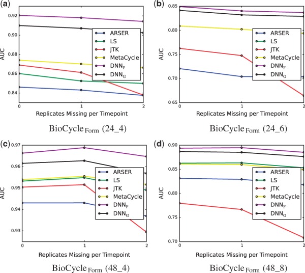
AUC at different levels of missing data

4.4 Time inference from single timepoint measurements

4.4.1 Overall performance

BIO_CLOCK is trained using 16 core clock genes: Arntl, Per1, Per2, Per3, Cyr1, Cry2, Nr1d1, Nr1d2, Bhlhe40, Bhlhe41, Dbp, Npas2, Tef, Fmo2, Lonrf3 and Tsc22d3. When trained and tested on all the data, using 70% of the data for training and the remaining 30% for testing, it accurately predicts the time of the experiment with a mean absolute error of 1.22 h (less than 75 min) (Table 6). We experimented also with training BIO_CLOCK with an even smaller number of genes. For example, using only Arntl, Per1, Per2, Per3, Cry1 and Cry2, produces a mean absolute error of 3.72 h. Adding Nr1d1 and Nr1d2 to this set reduces the mean absolute error to 1.65 h.

Table 6.

Cross organ mean absolute error (MAE) comparison of BIO_CLOCK

			Testing
		Liver	Brain	Set1	Set2	All
	Liver	1.21	5.18	3.78	4.77	3.78
Training	Brain	3.94	1.50	3.28	5.39	3.84
	Set1	4.06	4.25	2.03	4.69	3.58
	Set2	2.31	4.10	2.14	0.75	2.00
	All	1.28	1.66	1.49	0.70	1.22

4.4.2 Training and testing on different organs/tissues

Table 6 shows the mean absolute errors obtained when training BIO_CLOCK on data from certain organs/tissues and testing it on data from a different set of organs/tissues. All the data is from mice and under WT condition. The only datasets for which we have enough data for training correspond to liver and brain (when aggregating all the corresponding datasets). We form two additional sets (Set 1 and Set 2) by combining data from other organs. The first corresponds to combined data from the adrenal gland, fat, gut, kidney, lung and muscle (Set 1). The second corresponds to combined data from the aorta, colon, fibroblast, heart, macrophages and pituitary gland (Set 2). Finally, all of the aforementioned data is combined to form a bigger dataset (All). In all the experiments reported in Table 6, the data are split using a 70/30 training/test ratio, and tests sets never overlap with any of the corresponding training sets. The DNNs perform best when trained and tested on the same organ/tissue or sets of organ/tissues or when trained on all the organs/tissues. The DNNs perform significantly worse when trained and tested on data with diverging origins. However, in all cases, the DNN trained on the combined dataset does almost as well as, or better than, the corresponding specialized DNN.

4.4.3 Training and testing on different conditions

The collected data also includes data from mice under experimental conditions. The experimental conditions include high-fat and ketogenic diets, epilepsy and SIRT1 and SIRT6 knockouts. This dataset is too small to build a training and testing set. However, one can test the BIO_CLOCK DNN trained on the combined mice organs under normal conditions on this dataset. This experiment yields a mean absolute error of 2.57 h.

4.4.4 Annotation of the GEO database

Finally, we extract all the mouse gene expression experiments contained in the GEO repository (Edgar et al., 2002) and run BIO_CLOCK on them. A file containing all the corresponding imputed times is available from the CircadiOmics web portal.

5 Conclusion

Deep learning methods can be applied to high-throughput circadian data to address important challenges in circadian biology. In particular, we have developed BIO_CYCLE to detect molecular species that oscillate in high-throughput circadian experiments and extract the characteristics of these oscillations. Remarkably, BIO_CYCLE can be trained with large quantities of synthetic data preventing any kind of overfitting. We have also developed BIO_CLOCK to infer the time at which a transcriptomic sample was collected from the level of expression of a small number of core clock genes. Both methods will be improved as more data becomes available and, more generally, deep learning methods are likely to be useful to address several other related circadian problems, such as analyzing periodicity in high-throughput circadian proteomic data, or inferring sample time in different species. In particular, developing methods for annotating the time of all the human gene expression experiments, contained in GEO, and other similar repositories, would be valuable. Such annotations could be important for improving the interpretation of both old and new data and discovering circadian driven effects that may be important in precision medicine and other applications, for instance to help determine the optimal time for administering certain drugs.

References

- Allison D.B. et al. (2002) A mixture model approach for the analysis of microarray gene expression data. Comput. Stat. Data Anal., 39, 1–20. [Google Scholar]
- Andrews J.L. et al. (2010) Clock and bmal1 regulate myod and are necessary for maintenance of skeletal muscle phenotype and function. Proc. Natl. Acad. Sci. USA, 107, 19090–19095. [DOI] [PMC free article] [PubMed] [Google Scholar]
- Antunes L.C. et al. (2010) Obesity and shift work: chronobiological aspects. Nutr. Res. Rev., 23, 155–168. [DOI] [PubMed] [Google Scholar]
- Baldi P. (2012) Autoencoders, Unsupervised Learning, and Deep Architectures. J. Mach. Learn. Res., 27, 37–50 (Proceedings of 2011 ICML Workshop on Unsupervised and Transfer Learning). [Google Scholar]
- Baldi P., Sadowski P. (2014) The dropout learning algorithm. Artif. Intell., 210C, 78–122. [DOI] [PMC free article] [PubMed] [Google Scholar]
- Baldi P. et al. (2000) Assessing the accuracy of prediction algorithms for classification: an overview. Bioinformatics, 16, 412–424. [DOI] [PubMed] [Google Scholar]
- Baldi P. et al. (2014) Searching for exotic particles in high-energy physics with deep learning. Nat. Commun., 5, Article No. 4308. [DOI] [PubMed] [Google Scholar]
- Bellet M.M. et al. (2013) Circadian clock regulates the host response to salmonella. Proc. Natl. Acad. Sci., 110, 9897–9902. [DOI] [PMC free article] [PubMed] [Google Scholar]
- Benjamini Y., Hochberg Y. (1995) Controlling the false discovery rate: a practical and powerful approach to multiple testing. J. R. Stat. Soc. Ser. B (Methodological), 57, 289–300. [Google Scholar]
- Brown S.A. et al. (2012) (re)inventing the circadian feedback loop. Dev. Cell, 22, 477–487. [DOI] [PubMed] [Google Scholar]
- Covington M.F. et al. (2008) Global transcriptome analysis reveals circadian regulation of key pathways in plant growth and development. Genome Biol., 9, R130.. [DOI] [PMC free article] [PubMed] [Google Scholar]
- Deckard A. et al. (2013) Design and analysis of large-scale biological rhythm studies: a comparison of algorithms for detecting periodic signals in biological data. Bioinformatics, 29, 3174–3180. [DOI] [PMC free article] [PubMed] [Google Scholar]
- Di Lena P. et al. (2012) Deep architectures for protein contact map prediction. Bioinformatics, 28, 2449–2457. [DOI] [PMC free article] [PubMed] [Google Scholar]
- Dibner C. et al. (2010) The mammalian circadian timing system: organization and coordination of central and peripheral clocks. Annu. Rev. Physiol., 72, 517–549. [DOI] [PubMed] [Google Scholar]
- Duvenaud D. (2014). Automatic model construction with Gaussian processes. Ph.D. thesis, University of Cambridge.
- Dyar K.A. et al. (2014) Muscle insulin sensitivity and glucose metabolism are controlled by the intrinsic muscle clock. Mol. Metab., 3, 29–41. [DOI] [PMC free article] [PubMed] [Google Scholar]
- Eckel-Mahan K., Sassone-Corsi P. (2009) Metabolism control by the circadian clock and vice versa. Nat. Struct. Mol. Biol., 16, 462–467. [DOI] [PMC free article] [PubMed] [Google Scholar]
- Eckel-Mahan K.L. et al. (2008) Circadian oscillation of hippocampal mapk activity and camp: implications for memory persistence. Nat. Neurosci., 11, 1074–1082. [DOI] [PMC free article] [PubMed] [Google Scholar]
- Eckel-Mahan K.L. et al. (2012) Coordination of the transcriptome and metabolome by the circadian clock. Proc. Natl. Acad. Sci. USA, 109, 5541–5546. [DOI] [PMC free article] [PubMed] [Google Scholar]
- Eckel-Mahan K.L. et al. (2013) Reprogramming of the circadian clock by nutritional challenge. Cell, 155, 1464–1478. [DOI] [PMC free article] [PubMed] [Google Scholar]
- Edgar R. et al. (2002) Gene expression omnibus: NCBI gene expression and hybridization array data repository. Nucleic Acids Res., 30, 207–210. PMID: 11752295. [DOI] [PMC free article] [PubMed] [Google Scholar]
- Froy O. (2010) Metabolism and circadian rhythms – implications for obesity. Endocr. Rev., 31, 1–24. [DOI] [PubMed] [Google Scholar]
- Froy O. (2011) Circadian rhythms, aging, and life span in mammals. Physiology (Bethesda), 26, 225–235. [DOI] [PubMed] [Google Scholar]
- Gerstner J.R. et al. (2009) Cycling behavior and memory formation. J. Neurosci., 29, 12824–12830. [DOI] [PMC free article] [PubMed] [Google Scholar]
- Glynn E.F. et al. (2006) Detecting periodic patterns in unevenly spaced gene expression time series using lomb – scargle periodograms. Bioinformatics, 22, 310–316. [DOI] [PubMed] [Google Scholar]
- Goodfellow I.J. et al. (2013) Pylearn2: a machine learning research library. arXiv Preprint arXiv, 1308.4214. [Google Scholar]
- Hannun A. et al. (2014) Deepspeech: Scaling up end-to-end speech recognition. arXiv Preprint arXiv,. 1412.5567. [Google Scholar]
- Harmer S.L. et al. (2000) Orchestrated transcription of key pathways in arabidopsis by the circadian clock. Science, 290, 2110–2113. [DOI] [PubMed] [Google Scholar]
- Harmer S.L. et al. (2001) Molecular bases of circadian rhythms. Annu. Rev. Cell Devel. Biol., 17, 215–253. [DOI] [PubMed] [Google Scholar]
- Hughes M.E. et al. (2009) Harmonics of circadian gene transcription in mammals. PLoS Genet., 5, e1000442.. [DOI] [PMC free article] [PubMed] [Google Scholar]
- Hughes M.E. et al. (2010) Jtk_cycle: an efficient nonparametric algorithm for detecting rhythmic components in genome-scale data sets. J. Biol. Rhythms, 25, 372–380. [DOI] [PMC free article] [PubMed] [Google Scholar]
- Jia Y. et al. (2014) Caffe: Convolutional architecture for fast feature embedding. arXiv Preprint arXiv, 1408.5093. [Google Scholar]
- Karlsson B. et al. (2001) Is there an association between shift work and having a metabolic syndrome? Results from a population based study of 27,485 people. Occup. Environ. Med., 58, 747–752. [DOI] [PMC free article] [PubMed] [Google Scholar]
- Knutsson A. (2003) Health disorders of shift workers. Occup. Med. (Lond), 53, 103–108. [DOI] [PubMed] [Google Scholar]
- Kohsaka A. et al. (2007) High-fat diet disrupts behavioral and molecular circadian rhythms in mice. Cell Metab., 6, 414–421. [DOI] [PubMed] [Google Scholar]
- Kondratov R.V. et al. (2006) Early aging and age-related pathologies in mice deficient in bmal1, the core component of the circadian clock. Genes Devel., 20, 1868–1873. [DOI] [PMC free article] [PubMed] [Google Scholar]
- Lamia K.A. et al. (2008) Physiological significance of a peripheral tissue circadian clock. Proc. Natl. Acad. Sci. USA, 105, 15172–15177. [DOI] [PMC free article] [PubMed] [Google Scholar]
- Lenz I. et al. (2015) Deep learning for detecting robotic grasps. Int. J. Robot. Res., 34, 705–724. [Google Scholar]
- Liu G. et al. (2003) Netaffx: affymetrix probesets and annotations. Nucleic Acids Res., 31, 82–86. [DOI] [PMC free article] [PubMed] [Google Scholar]
- Lusci A. et al. (2013) Deep architectures and deep learning in chemoinformatics: the prediction of aqueous solubility for drug-like molecules. J. Chem. Inf. Model., 53, 1563–1575. [DOI] [PMC free article] [PubMed] [Google Scholar]
- Masri S. et al. (2013) Circadian acetylome reveals regulation of mitochondrial metabolic pathways. Proc. Natl. Acad. Sci., 110, 3339–3344. [DOI] [PMC free article] [PubMed] [Google Scholar]
- Masri S. et al. (2014a) Partitioning circadian transcription by sirt6 leads to segregated control of cellular metabolism. Cell, 158, 659–672. [DOI] [PMC free article] [PubMed] [Google Scholar]
- Masri S. et al. (2014b) SIRT6 defines circadian transcription leading to control of lipid metabolism. Cell, 158, 659–672. [DOI] [PMC free article] [PubMed] [Google Scholar]
- Miller B.H. et al. (2007) Circadian and clock-controlled regulation of the mouse transcriptome and cell proliferation. Proc. Natl. Acad. Sci. USA, 104, 3342–3347. [DOI] [PMC free article] [PubMed] [Google Scholar]
- Monnier A. et al. (2010) Orchestrated transcription of biological processes in the marine picoeukaryote ostreococcus exposed to light/dark cycles. BMC Genomics, 11, 192.. [DOI] [PMC free article] [PubMed] [Google Scholar]
- Moore R.Y., Eichler V.B. (1972) Loss of a circadian adrenal corticosterone rhythm following suprachiasmatic lesions in the rat. Brain Res., 42, 201–206. [DOI] [PubMed] [Google Scholar]
- Panda S. et al. (2002) Coordinated transcription of key pathways in the mouse by the circadian clock. Cell, 109, 307–320. [DOI] [PubMed] [Google Scholar]
- Partch C.L. et al. (2014) Molecular architecture of the mammalian circadian clock. Trends Cell Biol., 24, 90–99. [DOI] [PMC free article] [PubMed] [Google Scholar]
- Patel V. et al. (2012) Circadiomics: integrating circadian genomics, transcriptomics, proteomics, and metabolomics. Nat. Methods, 9, 772–773. [DOI] [PubMed] [Google Scholar]
- Patel V.R. et al. (2015) The pervasiveness and plasticity of circadian oscillations: the coupled circadian-oscillators framework. Bioinformatics, 31, 3181–3188. [DOI] [PMC free article] [PubMed] [Google Scholar]
- Pizarro A. et al. (2012) Circadb: a database of mammalian circadian gene expression profiles. Nucleic Acids Res, http://nar.oxfordjournals.org/content/early/2012/11/23/nar.gks1161.full. [DOI] [PMC free article] [PubMed] [Google Scholar]
- Quang D. et al. (2015) Dann: a deep learning approach for annotating the pathogenicity of genetic variants. Bioinformatics, 31, 761–763. [DOI] [PMC free article] [PubMed] [Google Scholar]
- Ralph M.R. et al. (1990) Transplanted suprachiasmatic nucleus determines circadian period. Science, 247, 975–978. [DOI] [PubMed] [Google Scholar]
- Rasmussen C.E. (2004) Gaussian Processes for Machine Learning. Advanced lectures on machine learning. Springer, Berlin Heidelberg, pp. 63–71. [Google Scholar]
- Rumelhart D.E. et al. (1988) Learning representations by back-propagating errors. Cognit. Model., 5, 3. [Google Scholar]
- Schibler U., Sassone-Corsi P. (2002) A web of circadian pacemakers. Cell, 111, 919–922. [DOI] [PubMed] [Google Scholar]
- Sharifian A. et al. (2005) Shift work as an oxidative stressor. J. Circadian Rhythms, 3, 15.. [DOI] [PMC free article] [PubMed] [Google Scholar]
- Shi S. et al. (2013) Circadian disruption leads to insulin resistance and obesity. Curr. Biol., 23, 372–381. [DOI] [PMC free article] [PubMed] [Google Scholar]
- Srivastava N. et al. (2014) Dropout: a simple way to prevent neural networks from overfitting. J. Mach. Learn. Res., 15, 1929–1958. [Google Scholar]
- Storch K.F. et al. (2002) Extensive and divergent circadian gene expression in liver and heart. Nature, 417, 78–83. [DOI] [PubMed] [Google Scholar]
- Stratmann M., Schibler U. (2006) Properties, entrainment, and physiological functions of mammalian peripheral oscillators. J. Biol. Rhythms, 21, 494–506. [DOI] [PubMed] [Google Scholar]
- Straume M. (2004) Dna microarray time series analysis: automated statistical assessment of circadian rhythms in gene expression patterning. Methods Enzymol., 383, 149–166. [DOI] [PubMed] [Google Scholar]
- Sutskever I. et al. (2013) On the importance of initialization and momentum in deep learning. In: Proceedings of the 30th International Conference on Machine Learning (ICML-13), pp. 1139–1147. [Google Scholar]
- Szegedy C. et al. (2014) Going deeper with convolutions. arXiv Preprint arXiv, 1409.4842. [Google Scholar]
- Takahashi J.S. et al. (2008) The genetics of mammalian circadian order and disorder: implications for physiology and disease. Nat. Rev. Genet., 9, 764–775. [DOI] [PMC free article] [PubMed] [Google Scholar]
- Turek F.W. et al. (2005) Obesity and metabolic syndrome in circadian clock mutant mice. Science, 308, 1043–1045. [DOI] [PMC free article] [PubMed] [Google Scholar]
- Vijayan V. et al. (2009) Oscillations in supercoiling drive circadian gene expression in cyanobacteria. Proc. Natl. Acad. Sci., 106, 22564–22568. [DOI] [PMC free article] [PubMed] [Google Scholar]
- Wu G. et al. (2016) Metacycle: An Integrated r Package to Evaluate Periodicity In Large Scale Data, Cold Spring Harbor Labs Journals. [DOI] [PMC free article] [PubMed] [Google Scholar]
- Yan J. et al. (2008) Analysis of gene regulatory networks in the mammalian circadian rhythm. PLoS Comput. Biol., 4, e1000193.. [DOI] [PMC free article] [PubMed] [Google Scholar]
- Yang R., Su Z. (2010) Analyzing circadian expression data by harmonic regression based on autoregressive spectral estimation. Bioinformatics, 26, i168–i174. [DOI] [PMC free article] [PubMed] [Google Scholar]
- Yoo S.H. et al. (2004) Period2::luciferase real-time reporting of circadian dynamics reveals persistent circadian oscillations in mouse peripheral tissues. Proc. Natl. Acad. Sci. USA, 101, 5339–5346. [DOI] [PMC free article] [PubMed] [Google Scholar]
- Zhang R. et al. (2014) A circadian gene expression atlas in mammals: Implications for biology and medicine. Proc. Natl. Acad. Sci., 111, 16219–16224. [DOI] [PMC free article] [PubMed] [Google Scholar]
Associated Data
This section collects any data citations, data availability statements, or supplementary materials included in this article.