A statistical model for brain networks inferred from large-scale electrophysiological signals

Abstract

Network science has been extensively developed to characterize the structural properties of complex systems, including brain networks inferred from neuroimaging data. As a result of the inference process, networks estimated from experimentally obtained biological data represent one instance of a larger number of realizations with similar intrinsic topology. A modelling approach is therefore needed to support statistical inference on the bottom-up local connectivity mechanisms influencing the formation of the estimated brain networks. Here, we adopted a statistical model based on exponential random graph models (ERGMs) to reproduce brain networks, or connectomes, estimated by spectral coherence between high-density electroencephalographic (EEG) signals. ERGMs are made up by different local graph metrics, whereas the parameters weight the respective contribution in explaining the observed network. We validated this approach in a dataset of N = 108 healthy subjects during eyes-open (EO) and eyes-closed (EC) resting-state conditions. Results showed that the tendency to form triangles and stars, reflecting clustering and node centrality, better explained the global properties of the EEG connectomes than other combinations of graph metrics. In particular, the synthetic networks generated by this model configuration replicated the characteristic differences found in real brain networks, with EO eliciting significantly higher segregation in the alpha frequency band (8–13 Hz) than EC. Furthermore, the fitted ERGM parameter values provided complementary information showing that clustering connections are significantly more represented from EC to EO in the alpha range, but also in the beta band (14–29 Hz), which is known to play a crucial role in cortical processing of visual input and externally oriented attention. Taken together, these findings support the current view of the functional segregation and integration of the brain in terms of modules and hubs, and provide a statistical approach to extract new information on the (re)organizational mechanisms in healthy and diseased brains.

1. Introduction

The study of the human brain at rest provides precious information that is predictive of intrinsic functioning, cognition, as well as pathology [1]. In the last decade, graph theoretic approaches have described the topological structure of resting-state connectomes derived from different neuroimaging techniques, such as functional magnetic resonance imaging (fMRI) or magneto- (MEG) and electroencephalography (EEG).

These estimated connectomes, or brain networks, tend to exhibit similar organizational properties, including small-worldness, cost-efficiency, modularity and node centrality [2], as well as characteristic dependence from the anatomical backbone connectivity [3–5] and genetic factors [6]. Furthermore, they potentially show clinical relevance, as demonstrated by the recent development of network-based diagnostics of consciousness [7,8], Alzheimer's disease [9], stroke recovery [10] and schizophrenia [11]. In this sense, quantifying the topological properties of intrinsic functional connectomes by means of graph theory has enriched our understanding of the structure of functional brain connectivity maps [2,12–14]. Nevertheless, these results refer to a descriptive analysis of the observed brain network, which is only one instance of several alternatives with similar structural features. This is especially true for functional networks inferred from empirically obtained data, where the edges (or links) are noisy estimates of the true connectivity and thresholding is often adopted to filter the relevant interactions between the system units [15–17].

Statistical models are, therefore, needed to reflect the uncertainty associated with a given observation, to permit inference about the relative occurrence of specific local structures and to relate local-level processes to global-level properties [18]. A first approach consists in generating synthetic random networks that preserve some observed properties, such as the degree distribution or the random walk distribution, and then contrasting the values of the graph indices obtained in these synthetic networks with those extracted from the estimated connectomes [13]. While these methods often provide appropriate null models, and can improve the identification of relevant network properties [19–21], they do not inform on the organizational mechanisms modelling the whole network formation [22,23]. Alternative approaches consider probabilistic growth models such as those based on spatial distances between nodes [24]. Interesting results have been achieved in identifying some basic connectivity rules reproducing both structural and functional brain networks [25,26]. However, these methods suffer from the rough approximation (e.g. Euclidean) of the actual spatial distance between nodes, and, moreover, they do not indicate whether the identified local mechanisms are either necessary or sufficient as descriptors of the global network structure.

To support inference on the processes influencing the formation of network structure, statistical models have been conceived to consider the set of all possible alternative networks weighted on their similarity to the observed one [18]. Among others, exponential random graph models (ERGMs) represent a flexible category that allows the simultaneous assessment of the role of specific graph features in the formation of the entire network. These models were first proposed as an extension of the triad model defined in [27] to characterize Markov graphs [28,29] and have been widely developed to understand how simple interaction rules, such as transitivity, could give rise to the complex network of social contacts [30–38].

Recently, the use of ERGMs has been proved to successfully model imaging connectomes derived respectively from spontaneous fMRI activity [39] and diffusion tensor imaging (DTI) [40]. Despite its potential, the use of ERGMs in network neuroscience is still in its infancy and more evidence is needed to better elucidate its applicability to connectomes inferred from other types of neuroimaging data and across different experimental conditions. In addition, many methodological issues remain unanswered, such as the relationships between the graph metrics included in the ERGM and the graph indices used to describe the topology of the observed connectomes.

To address the above issues, we proposed and evaluated several ERGM configurations based on the combination of different local connectivity structures (i.e. graph metrics). Specifically, we modelled brain networks estimated from high-density EEG signals in a group of healthy individuals during eyes-open (EO) and eyes-closed (EC) resting states. Our goal was to identify the best ERGM configuration reproducing EEG-derived connectomes in terms of functional integration and segregation, and to evaluate the ability of the estimated ERGM parameters in providing new information discriminating between EO and EC conditions.

2. Material and methods

2.1. Electroencephalographic data and brain network construction

We used high-density EEG signals freely available from the online PhysioNet BCI database [41,42]. EEG data consisted of 1 min resting state with EO and 1 min resting state with EC recorded from 56 electrodes in 108 healthy subjects. EEG signals were recorded with an original sampling rate of 160 Hz. All the EEG signals were referenced to the mean signal gathered from electrodes on the ear lobes. We subsequently downsampled the EEG signals to 100 Hz after applying a proper anti-aliasing low-pass filter. The electrode positions on the scalp followed the standard 10–10 montage.

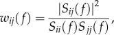
We used the spectral coherence [43] to measure functional connectivity (FC) between EEG signals of sensors i and j at a specific frequency band f as follows:

2.1

where S_ij is the cross-spectrum between i and j, and S_ii and S_jj are the autospectra of i and j, respectively. Specifically, we computed cross- and auto-spectra by means of Welch's averaged modified periodogram with a sliding Hanning window of 1 s and 0.5 s of overlap. The number of fast Fourier transform points was set to 100 for a frequency resolution of 1 Hz. As a result, we obtained for each subject a connectivity matrix W(f) of size 56 × 56 where the entry w_ij(f) contains the value of the spectral coherence between the EEG signals of sensors i and j at the frequency f.

We then averaged the connectivity matrices within the characteristic frequency bands theta (4–7 Hz), alpha (8–13 Hz), beta (14–29 Hz) and gamma (30–40 Hz). These matrices constituted our raw brain networks whose nodes corresponded to the EEG sensors (n = 56) and links corresponded to the w_ij values. Finally, we thresholded the values in the connectivity matrices to retain the strongest links in each brain network. Specifically, we adopted an objective criterion, i.e. the efficiency cost optimization (ECO), to filter and binarize a number of links such that the final average node degree k = 3 [44]. We also considered k = 1, 2, 4, 5 to evaluate the main brain network properties around the representative threshold k = 3. The resulting sparse brain networks, or graphs, were represented by adjacency matrices A, where each entry indicates the presence a_ij = 1 or the absence a_ij = 0 of a link between nodes i and j.

2.2. Graph indices

We evaluated the global structure of brain networks by measuring graph indices at large-scale topological scales. We focused on well-known properties of brain networks such as optimal balance between integration and segregation of information [2,45,46]. Integration is the tendency of the network to favour distributed connectivity among remote brain areas; conversely, segregation is the tendency of the network to maintain connectivity within specialized groups of brain areas [47].

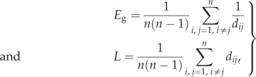
In graph theory, integration has been typically quantified by the global-efficiency E_g and by the characteristic path length L,

2.2

where d_ij is the distance, or the length of the shortest path, between nodes i and j [48,49].

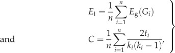
Segregation is typically measured by means of the local-efficiency E_l and by the clustering coefficient C:

2.3

where G_i is the subgraph formed by the nodes connected to i; t_i is the number of triangles around node i; and k_i is the degree of node i [48,49].

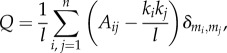
In addition, we evaluated the strength of division of a network into modules by measuring the modularity Q:

2.4

where 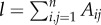is the number of edges, m_i is the module containing node i and δ_mi,mj = 1 if m_i = m_j and 0 otherwise. We used the Walktrap algorithm to generate a sequence of community partitions [50] and we selected the one that maximized Q according to the standard algorithm proposed in [51]. Modularity can be seen as a compact measure of the integration and segregation of a network, as it measures the propensity to form dense connections between nodes within modules (i.e. segregation) but sparse connections between nodes in different modules (i.e. inverse of integration).

2.3. Exponential random graph model

Let G be a graph in a set of possible network realizations, g = [g₁, g₂, … , g_r] be a vector of graph statistics, or metrics, and g* = [g*₁, g*₂, … , g*_r] be the values of these metrics measured over G. Then, we can statistically model G by defining a probability distribution P(G) over such that the following conditions are satisfied:

2.5

and

2.6

where 〈g_i〉 is the expected value of the ith graph metric over .

By maximizing the Gibbs entropy of P(G) constrained to the above conditions, the probability distribution reads as:

2.7

where 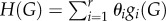is the graph Hamiltonian, θ_i is the ith model parameter to be estimated and 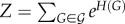is the so-called partition function [52]. The estimated value of a parameter θ_i indicates the change in the (log-odds) likelihood of an edge for a unit change in graph metric g_i. If the estimated value of θ_i is large and positive, the associated graph metric g_i plays an important role in explaining the topology of G more than would be expected by chance. Note that here chance corresponds to randomly choosing a network from the space . If instead the estimated value of θ_i is negative and large, then g_i still plays an important role in explaining the topology of G but it is less prevalent than expected by chance [53].

In general, the fact that the space can be very large even for relatively small n, as well as the inclusion of graph metrics that are not simple linear combinations of G_ij, in practice make it impossible to derive analytically the model parameters vector θ = [θ₁, θ₂, … , θ_r] [27,31].

Numerical methods, such as Markov chain Monte Carlo (MCMC) approximations of the maximum-likelihood estimators (MLEs) of the model parameters vector θ, are typically adopted to circumvent this issue [54].

2.3.1. Model construction and implementation

We considered graph metrics reflecting the basic properties of complex systems such as hub propensity and transitivity in the network [46,55,56]. Specifically, we focused on k-stars to model highly connected nodes (hubs) and k-triangles to model transitivity, where k refers to the order of the structures as illustrated in figure 1.

Figure 1.

Graphical representation of k-stars and k-triangles.

In general, this leads to a large number of model parameters to be estimated, i.e. n − 1 for k-stars and n − 2 for k-triangles. To avoid consequent degeneracy issues in the ERGM estimation, we adopted a compact specification for these metrics that combines them in an alternating geometric sequence [31,57].

Because k-stars are related to the node degree distribution D [33], we used the geometrically weighted degree distribution GW_K as a graph metric to characterize hub propensity:

2.8

where τ > 0 is a ratio parameter to penalize nodes with extremely high node degrees.

Similarly, because k-triangles are related to the shared pattern distribution S, we used the geometrically weighted edgewise shared partner distribution to characterize transitivity:

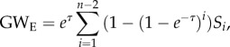2.9

where the element S_i is the number of dyads that are directly connected and that have exactly i neighbours in common.

In addition, complementary metrics have been defined based on the shared partner distribution:

• GW_N: geometrically weighted non-edgewise shared partner distribution given by equation (2.9), with S_i considering exclusively dyads that are not connected.

• GW_D: geometrically weighted dyadwise shared partner distribution given by equation (2.9), with S_i considering any dyad, connected or not.

The above specifications yield particular ERGMs that belong to the so-called curved exponential family [33] and that have been extensively used in social science [32,58,59].

We constructed different ERGM configurations by including these graph metrics as illustrated in table 1. For the sake of simplicity, we only considered combinations of two graph metrics at most, except in one case where we also included the number of edges as a further metric [39,40].

Table 1.

Set of model configurations. Models M₁–M₁₀ include at most two of the four considered graph metrics, i.e. GW_K, GW_E, GW_N, GW_D. The metric ‘edges’ is fixed and equal to the actual number of edges in the observed brain networks in all the configurations but M₁₁ model. *Metrics that are fixed. ✓Metrics that are variable.

models	edges	GWK	GWE	GWN	GWD
M1	*	✓	✓	–	—
M2	*	—	✓	—	✓
M3	*	—	—	✓	✓
M4	*	—	✓	✓	—
M5	*	—	✓	—	—
M6	*	—	—	✓	—
M7	*	✓	—	✓	—
M8	*	✓	—	—	✓
M9	*	✓	—	—	—
M10	*	—	—	—	✓
M11	✓	—	✓	✓	—

We tested the different configurations by fitting the ERGM to brain networks in each single subject (N = 108), frequency band (theta, alpha, beta, gamma) and condition (EO, EC). To fit ERGMs, we used an MCMC algorithm (Gibbs sampler) that samples networks from an exponential graph distribution. Specifically, we set the initial values of the model parameters θ⁰ by means of a maximum pseudo-likelihood estimation (MPLE) [54,60]. Then, we adopted Fisher's scoring method to update the model parameters θ until they converged to the approximated MLEs [31]. As we used curved ERGMs, the ratio parameters τ were not fixed but were estimated.

Eventually, for each fitted ERGM configuration we generated 100 synthetic networks in order to obtain appropriate confidence intervals.

2.3.2. Goodness of fit

First, we used the Akaike information criterion (AIC) to evaluate the relative quality of the ERGMs' fit by taking into account the maximum value of the likelihood function and the number of model parameters [61].

We also adopted a different approach to assess the absolute quality of the fit by comparing the synthetic networks generated by the estimated ERGMs and the observed brain networks. Specifically, we defined the following score based on the integration and segregation properties of networks:

2.10

where η_Eg,η_El are the relative errors between the mean values of the global/local efficiency of the simulated networks and the value of the observed brain network. By selecting the maximum absolute error, we were considering the worst case, similar to what was proposed in [26]. Based on the above criteria, we selected the best model, which minimizes the AIC and δ mean values. To validate the model adequacy (equation (2.6)), we computed the Z-scores between the graph metrics' values of brain networks and synthetic networks.

Furthermore, we cross-validated the best model configuration by evaluating the synthetic networks' fit to graph indices that were explicitly not included in either the ERGM or the model selection criteria. We computed Pearson's correlation coefficient between the values of the characteristic path length (L), clustering coefficient (C) and modularity (Q) extracted from the observed brain networks and the mean values obtained from the corresponding simulated networks. In addition, we used the Mirkin index (MI) [62] to evaluate the similarity between the community partitions of the observed networks and the consensus partitions of the corresponding synthetic networks.

2.4. Statistical group analysis

We assessed the statistical differences between the values of the graph indices extracted from the brain networks in the EO and EC resting-state conditions. We also computed between-condition differences using the synthetic networks fitted by the best ERGM. In this case, we considered the mean values of the graph indices in order to have one value corresponding to one brain network. Eventually, we computed the statistical differences between the values of the best ERGM parameters in the EO and EC conditions in order to assess their potential to provide complementary information to that provided by standard graph analysis. For each comparison, we used a non-parametric permutation t-test and we fixed a statistical threshold of α = 0.001 and 100 000 permutations.

3. Results

3.1. Characteristic functional segregation of electroencephalographic resting-state networks

The group analysis revealed a significant increase in the local-efficiency in EO, compared with that in EC, for the alpha band (T = 3.529, p = 0.0007, figure 2). We also reported a significant increment (T = 3.557, p = 0.0007) for the modularity in the alpha band, while no other statistically significant differences were observed in the other frequency bands, graph indices or metrics (electronic supplementary material, table S3).

Figure 2.

Median values and standard errors of global- and local-efficiency measured from EEG brain networks across 108 subjects in eyes-open (EO) and eyes-closed (EC) resting states. *p-value < 0.001.

These differences were obtained for brain networks thresholded with an average node degree k = 3 according to the ECO criterion [44]. We reported a similar increase in functional segregation (local-efficiency) in the alpha band for k = 5 (electronic supplementary material, figure S1). More details on the analysis for k = 5 can be found in the electronic supplementary material (Supp_text.pdf).

In terms of existing relationships between graph indices and ERGM metrics, we could not establish univocal associations between E_g and E_l values and the metrics' values used in the ERGMs (electronic supplementary material, table S1). This was especially true for the global-efficiency, which exhibited significantly high correlations with all the other graph metrics (Spearman's |R| > 0.43, p < 10⁻³⁹).

3.2. Triangles and stars as fundamental constituents of functional brain networks

All the proposed ERGM configurations exhibited a relatively good fitting in terms of AIC, except for M₁₁ (electronic supplementary material, figure S2). Notably, the latter was the only configuration where the number of edges was considered as a model parameter and not as a constraint. M₁ gave the lowest δ(E_g, E_l) scores compared with the other configurations in both the EO and EC conditions (figure 3). Notably, the configurations giving lower δ(E_g, E_l) scores included, directly or indirectly, the metric GW_E, with the exception of M₁₁.

Figure 3.

Absolute quality of the fit of ERGMs. Coloured bars show the group-averaged cumulative errors δ(E_g, E_l) in terms of the relative of global- and local-efficiency across frequency bands. Model configurations are listed on the x-axis. (a) Values for the eyes-open resting state (EO); (b) the error values for the eyes-closed resting state (EC). (Online version in colour.)

We selected M₁ as a potentially good candidate to model EEG-derived brain networks. According to this model configuration the mass probability density reads . The group-median values of the estimated parameters (θ₁ and θ₂) were all positive and larger than 1 in each band and condition (table 2). This means that the likelihood of an edge existing in a simulated network is larger if that edge is part of a triangle (GW_E) or of a star (GW_K), and that these connectivity structures are statistically relevant for the brain network formation.

Table 2.

Statistics for the estimated parameters of the model configuration M₁. Median values and standard errors (within parentheses) are reported for the two resting-state conditions EO and EC. t-values and p-values (within parentheses) from non-parametric permutation-based t-tests between EO and EC are shown in the third column of each subsection marked with the heading EO − EC.

	θ1			θ2
	EO	EC	EO − EC	EO	EC	EO − EC
theta	1.528 (0.045)	1.531 (0.039)	−0.281 (0.7804)	1.502 (0.169)	1.443 (0.159)	−0.406 (0.690)
alpha	1.449 (0.041)	1.297 (0.039)	3.746 (0.0002)	1.327 (0.123)	1.317 (0.532)	−1.084 (0.347)
beta	1.487 (0.457)	1.326 (0.046)	1.514 (0.0009)	1.062 (0.149)	1.303 (0.169)	−0.890 (0.371)
gamma	1.552 (0.046)	1.509 (8.266)	−0.992 (0.8521)	0.878 (0.125)	1.140 (3.002)	−1.064 (0.135)

Overall, the GW_E and GW_K values of the synthetic networks generated by M₁ were not significantly different from those of the observed brain networks (figure 4). This was true in every subject for GW_E (Z < 2.58, p > 0.01) and in at least 94% of the subjects for GW_E (Z < 2.58, p > 0.01). Furthermore, the values of the characteristic path length (L), clustering coefficient (C) and modularity (Q) extracted from synthetic networks were significantly correlated (Pearson's R > 0.44, p < 10⁻⁶) with those of the brain networks in each frequency band (figure 5; electronic supplementary material, table S2). In addition, synthetic networks exhibited a similar community partition to individual brain networks, as revealed by the low MI values (MI < 0.21) (electronic supplementary material, figure S3). These results confirmed that M₁ adequately models the obtained EEG brain networks.

Figure 4.

Adequacy of the model configuration M₁. Green and red dots represent, respectively, the values of the geometrically weighted edgewise shared pattern distribution (GW_E) and the geometrically weighted degree distribution (GW_K) measured in simulated networks. Black dot lines indicate the values measured in the observed brain networks.

Figure 5.

Cross-validation for the model configuration M₁. Scatter plots show the values of the graph indices measured in the observed brain networks (x-axis) against the mean values obtained from synthetic networks (y-axis). Three graph indices were considered: characteristic path length (L), clustering coefficient (C) and modularity (Q). Grey dots correspond to eyes-open resting states (EO); black dots correspond to eyes-closed resting states (EC).

3.3. Simulating network differences between absence and presence of visual input

Figure 6 illustrates the brain networks for a representative subject in the alpha band along with the corresponding synthetic networks generated by M₁. In both the EO and EC conditions, simulated networks and brain networks share similar topological structures characterized by diffused regularity and more concentrated connectivity in parietal and occipital regions.

Figure 6.

Brain networks and synthetic networks for a representative subject. (a) Brain network in the alpha band for the eyes-open (EO) and eyes-closed (EC) resting state. (b) One instance of the corresponding synthetic networks generated by the model configuration M₁. (c) Because node labels are not preserved in the simulated networks, we re-assigned them virtually by using the Frank–Wolfe algorithm [63], which optimizes the graph matching with the observed brain network. In the upper part of the figure, nodes correspond to EEG electrodes, whose position follows a standard 10–10 montage. In the bottom part, the nodes are arranged into a circle. (Online version in colour.)

The group analysis over the synthetic networks revealed the ability of M₁ to capture not only the individual properties of brain networks but also the main observed difference between the EC and EO resting states, reflecting, respectively, the absence and presence of visual input. Similarly to observed brain networks, we obtained, for simulated networks, a marginally significant increase in the local-efficiency from EC to EO, in the alpha band (T = 3.168, p = 0.002). No other significant differences were reported in any other band or graph index/metric (electronic supplementary material, table S3).

Finally, by looking at the values of the estimated parameters, we observed that θ₁ values were significantly larger in EO than in EC for both the alpha (T = 3.746, p = 0.0002) and beta (Z = 1.514, p = 0.0009) frequency bands, while no significant differences were found for θ₂ values (table 2).

4. Discussion

In recent years, the use of statistical methods to infer the structure of complex systems has gained increasing interest [39,64–66]. Beyond the descriptive characterization of networks, statistical network models aim to statistically assess the local connectivity processes involved in the global structure formation [18]. This is a crucial advance with respect to standard descriptive approaches because imaging connectomes, as with other biological networks, is often inferred from experimentally obtained data and therefore the estimated edges can suffer from statistical noise and uncertainty [67].

In our study, we used ERGMs to identify the local connectivity structures that statistically form the intrinsic synchronization of large-scale electrophysiological activities. This model formulation has the advantage of statistically inferring the probability of edge formation accounting for highly dependent configurations, such as transitivity structures, something that is lacking in, for example, the Bernoulli model. Furthermore, it is possible to include, in theory, graph metrics measuring global and local properties and discriminating node and edges attributes, such as homophily effects. In addition, it generalizes well-known network models such as the stochastic block model, where a block structure is imposed by including the count of edges between groups of nodes as a model metric [68].

Here, the results showed that the tendency to form triangles (GW_E) and stars (GW_K) was sufficient to statistically reproduce the main properties of the EEG brain networks, such as functional integration and segregation, measured by means of global-efficiency E_g and local-efficiency E_l (electronic supplementary material, table S3). Our findings partially deviate from previous studies, which have used ERGMs to model fMRI and DTI brain networks, where GW_E and the geometrically weighted non-edgewise shared partner GW_N were selected under the assumption that these could be related, respectively, to local- and global-efficiency [39,40]. However, here we showed that a univocal relationship between the ERGM graph indices and the metrics used to describe the EEG connectomes could not be statistically established (electronic supplementary material, table S1). While the propensity to form triangles (GW_E) can lead to cohesive clustering in the network (E_l), the propensity to form redundant paths of length 2 (i.e. GW_N) is not clearly related to the formation of short paths between nodes (E_g) [57]. Thus, while in general a good fit can be achieved by including GW_N in the ERGM, the subsequent interpretation in terms of brain functional integration appears less straightforward. Here, we showed that GW_E together with the tendency to form stars (GW_K) gave the best fit in terms of local- and global efficiency. Triangles and stars, giving rise to clustering and hubs, are fundamental building blocks of complex systems reflecting important mechanisms such as transitivity [48] and preferential attachment [69]. Notably, the existence of highly connected nodes is compatible with the presence of short paths (e.g. in a star graph the characteristic path length L = 2). This supports the recent view of brain functional integration where segregated modules exchange information through central hubs and not necessarily through the shortest paths [70,71].

In the cross-validation phase, the selected model configuration captured other important brain network properties as measured by the clustering coefficient C, the characteristic path length L and the modularity Q (figure 5). In terms of the differences between conditions, the simulated networks gave a marginally significant increase (p = 0.002) in E_l in the alpha band during EO as compared with EC, while, differently from observed brain networks, no significant differences were reported for the modularity Q (electronic supplementary material, table S3). The latter could be, in part, ascribed to the absence of specific metrics in the ERGM accounting for modularity. In this respect, stochastic block models, which explicitly force modular structures, could represent an interesting alternative to explore in the future [72,73]. Here, the increased alpha local-efficiency suggests a modulation of augmented specialized information processing, from EC to EO, that is consistent with typical global power reduction and increased regional activity [74]. Possible neural mechanisms explaining this effect have been associated with the automatic gathering of non-specific information resulting from more interactions within the visual system [75] and with shifts from interoceptive towards exteroceptive states [76–78].

As a crucial result, we provided complementary information by inspecting the fitted ERGM parameters. The positive θ₁ > 1 and θ₂ > 1 values indicated that both GW_E and GW_K are fundamental connectivity features that emerge in brain networks more than expected by chance (table 2). However, only θ₁ values showed a significant difference (EO > EC) in the alpha band, as well as in the beta band (table 2), suggesting that the tendency to form triangles, rather than the tendency to form stars, is a discriminating feature of EO and EC modes. More concentrated EEG activity among parieto-occipital areas has been largely documented in the alpha and also in the beta bands, the latter reflecting either cortical processing of visual input or externally oriented attention [74,79]. Notably, the role of the beta band could not be found when analysing either brain networks or synthetic networks (figure 2; electronic supplementary material, table S3) and we speculate that this result specifically stems from the inherent ability of ERGMs to account for potential interaction between different graph metrics [57].

4.1. Methodological considerations

We estimated EEG connectomes by means of spectral coherence. While this measure is known to suffer from possible volume conduction effects [80], it has also been demonstrated that, probably due to this effect, it has the advantage of generating connectivity matrices that are highly consistent within and between subjects [81]. In addition, spectral coherence is still one of the most used measures to infer FC in the electrophysiological literature on resting states because of its simplicity and relatively intuitive interpretation. Thus, constructing EEG connectomes by means of spectral coherence allowed us to better contextualize the results obtained with ERGM from a neurophysiological perspective. Future studies will have to assess if and how different connectivity estimators affect the choice of the model parameters.

We used a density-based thresholding procedure to filter information in the EEG raw networks by retaining and binarizing the strongest edges. Despite the consequent information loss, thresholding is often adopted to mitigate the uncertainty of the weakest edges, reduce the false positives and facilitate the interpretation of the inferred network topology [13,17].

Selecting a binarizing threshold does have an impact on the topological structure of brain networks [82]. Based on the optimization of fundamental properties of complex systems, i.e. efficiency and economy, the adopted thresholding criterion (ECO) leads to sparse networks, with an average node degree k = 3, causing possible nodes to be disconnected. However, it has demonstrated empirically that the size of the resulting largest component typically contains more than 60% of the brain nodes, thus ensuring a sparse but meaningful network structure [44]. In a separate analysis, we verified that the validity of the model and the characteristic between-condition differences observed in the alpha band were also globally preserved for k = 5 (electronic supplementary material, Supp_text.pdf).

Authors' contributions

C.O. and F.D.V.F. both designed the study; C.O. performed the analysis and wrote the paper; and F.D.V.F. wrote the paper.

Competing interests

We declare we have no competing interests.

Funding

This work has been partially supported by the Agence Nationale de la Recherche (French programme) ANR-10-IAIHU-06 and ANR-15-NEUC-0006-02.

References

- 1.Raichle ME, MacLeod AM, Snyder AZ, Powers WJ, Gusnard DA, Shulman GL. 2001. A default mode of brain function. Proc. Natl Acad. Sci. USA 98, 676–682. ( 10.1073/pnas.98.2.676) [DOI] [PMC free article] [PubMed] [Google Scholar]
- 2.Bullmore E, Bullmore E, Sporns O, Sporns O. 2009. Complex brain networks: graph theoretical analysis of structural and functional systems. Nat. Rev. Neurosci. 10, 186–198. ( 10.1038/nrn2575) [DOI] [PubMed] [Google Scholar]
- 3.Honey CJ, Sporns O, Cammoun L, Gigandet X, Thiran JP, Meuli R, Hagmann P. 2009. Predicting human resting-state functional connectivity from structural connectivity. Proc. Natl Acad. Sci. USA 106, 2035–2040. ( 10.1073/pnas.0811168106) [DOI] [PMC free article] [PubMed] [Google Scholar]
- 4.Deco G, Ponce-Alvarez A, Mantini D, Romani GL, Hagmann P, Corbetta M. 2013. Resting-state functional connectivity emerges from structurally and dynamically shaped slow linear fluctuations. J. Neurosci. 33, 11239–11252. ( 10.1523/JNEUROSCI.1091-13.2013) [DOI] [PMC free article] [PubMed] [Google Scholar]
- 5.Park H-J, Friston K. 2013. Structural and functional brain networks: from connections to cognition. Science 342, 1238411 ( 10.1126/science.1238411) [DOI] [PubMed] [Google Scholar]
- 6.Fornito A. et al 2011. Genetic influences on cost-efficient organization of human cortical functional networks. J. Neurosci. 31, 3261–3270. ( 10.1523/JNEUROSCI.4858-10.2011) [DOI] [PMC free article] [PubMed] [Google Scholar]
- 7.Achard S, Delon-Martin C, Vértes PE, Renard F, Schenck M, Schneider F, Heinrich C, Kremer S, Bullmore ET. 2012. Hubs of brain functional networks are radically reorganized in comatose patients. Proc. Natl Acad. Sci. USA 109, 20 608–20 613. ( 10.1073/pnas.1208933109) [DOI] [PMC free article] [PubMed] [Google Scholar]
- 8.Chennu S. et al. 2014. Spectral signatures of reorganised brain networks in disorders of consciousness. PLoS Comput. Biol. 10, e1003887 ( 10.1371/journal.pcbi.1003887) [DOI] [PMC free article] [PubMed] [Google Scholar]
- 9.Tijms BM, Wink AM, de Haan W, van der Flier WM, Stam CJ, Scheltens P, Barkhof F. 2013. Alzheimer's disease: connecting findings from graph theoretical studies of brain networks. Neurobiol. Aging 34, 2023–2036. ( 10.1016/j.neurobiolaging.2013.02.020) [DOI] [PubMed] [Google Scholar]
- 10.Grefkes C, Fink GR. 2011. Reorganization of cerebral networks after stroke: new insights from neuroimaging with connectivity approaches. Brain 134, 1264–1276. ( 10.1093/brain/awr033) [DOI] [PMC free article] [PubMed] [Google Scholar]
- 11.Lynall M-E, Bassett DS, Kerwin R, McKenna PJ, Kitzbichler M, Muller U, Bullmore E. 2010. Functional connectivity and brain networks in schizophrenia. J. Neurosci. 30, 9477–9487. ( 10.1523/JNEUROSCI.0333-10.2010) [DOI] [PMC free article] [PubMed] [Google Scholar]
- 12.Stam C. 2004. Functional connectivity patterns of human magnetoencephalographic recordings: a ‘small-world’ network? Neurosci. Lett. 355, 25–28. ( 10.1016/j.neulet.2003.10.063) [DOI] [PubMed] [Google Scholar]
- 13.Rubinov M, Sporns O. 2010. Complex network measures of brain connectivity: uses and interpretations. NeuroImage 52, 1059–1069. ( 10.1016/j.neuroimage.2009.10.003) [DOI] [PubMed] [Google Scholar]
- 14.Stam CJ, van Straaten ECW. 2012. The organization of physiological brain networks. Clin. Neurophysiol. 123, 1067–1087. ( 10.1016/j.clinph.2012.01.011) [DOI] [PubMed] [Google Scholar]
- 15.Tumminello M, Aste T, Matteo TD, Mantegna RN. 2005. A tool for filtering information in complex systems. Proc. Natl Acad. Sci. USA 102, 10 421–10 426. ( 10.1073/pnas.0500298102) [DOI] [PMC free article] [PubMed] [Google Scholar]
- 16.Vidal M, Cusick M, Barabási A-L. 2011. Interactome networks and human disease. Cell 144, 986–998. ( 10.1016/j.cell.2011.02.016) [DOI] [PMC free article] [PubMed] [Google Scholar]
- 17.De Vico Fallani F, Richiardi J, Chavez M, Achard S. 2014. Graph analysis of functional brain networks: practical issues in translational neuroscience. Phil. Trans. R. Soc. B 369, 20130521 ( 10.1098/rstb.2013.0521) [DOI] [PMC free article] [PubMed] [Google Scholar]
- 18.Goldenberg A, Zheng AX, Fienberg SE, Airoldi EM. A survey of statistical network models. (http://arxiv.org/abs/0912.5410)
- 19.Milo R, Shen-Orr S, Itzkovitz S, Kashtan N, Chklovskii D, Alon U. 2002. Network motifs: simple building blocks of complex networks. Science 298, 824–827. ( 10.1126/science.298.5594.824) [DOI] [PubMed] [Google Scholar]
- 20.Garlaschelli D, Loffredo MI. Patterns of link reciprocity in directed networks. Phys. Rev. Lett. 93, 268701 ( 10.1103/PhysRevLett.93.268701) [DOI] [PubMed] [Google Scholar]
- 21.Humphries MD, Gurney K. 2008. Network ‘small-world-ness’: a quantitative method for determining canonical network equivalence. PLoS ONE 3, e0002051 ( 10.1371/journal.pone.0002051) [DOI] [PMC free article] [PubMed] [Google Scholar]
- 22.Barabasi A-L, Jeong H, Néda Z, Ravasz E, Schubert A, Vicsek T. 2002. Evolution of the social network of scientific collaborations. Physica A 311, 590–614. ( 10.1016/S0378-4371(02)00736-7) [DOI] [Google Scholar]
- 23.Newman MEJ, Watts DJ, Strogatz SH. 2002. Random graph models of social networks. Proc. Natl Acad. Sci. USA 99, 2566–2572. ( 10.1073/pnas.012582999) [DOI] [PMC free article] [PubMed] [Google Scholar]
- 24.Barthélemy M. 2011. Spatial networks. Phys. Rep. 499, 1–101. ( 10.1016/j.physrep.2010.11.002) [DOI] [Google Scholar]
- 25.Vertes PE, Alexander-Bloch AF, Gogtay N, Giedd JN, Rapoport JL, Bullmore ET. 2012. Simple models of human brain functional networks. Proc. Natl Acad. Sci. USA 109, 5868–5873. ( 10.1073/pnas.1111738109) [DOI] [PMC free article] [PubMed] [Google Scholar]
- 26.Betzel RF, et al 2016. Generative models of the human connectome. NeuroImage A 124, 1054–1064. ( 10.1016/j.neuroimage.2015.09.041) [DOI] [PMC free article] [PubMed] [Google Scholar]
- 27.Frank O, Strauss D. 1986. Markov graphs. J. Am. Stat. 81, 832–842. ( 10.2307/2289017) [DOI] [Google Scholar]
- 28.Frank O. 1991. Statistical analysis of change in networks. Stat. Neerland. 45, 283–293. ( 10.1111/j.1467-9574.1991.tb01310.x) [DOI] [Google Scholar]
- 29.Wasserman S, Pattison P. 1996. Logit models and logistic regressions for social networks: I. An introduction to Markov graphs and p. Psychometrika 61, 401–425. ( 10.1007/BF02294547) [DOI] [Google Scholar]
- 30.Handcock MS. 2002. Statistical models for social networks: inference and degeneracy. In Dynamic social network modeling and analysis (eds R Breiger, K Corley, P Pattison), pp. 229–240. Washington, DC: National Academies Press. [Google Scholar]
- 31.Hunter DR, Handcock MS. 2006. Inference in curved exponential family models for networks. J. Comput. Graph. Stat. 15, 565–583. ( 10.1198/106186006X133069) [DOI] [Google Scholar]
- 32.Goodreau SM. 2007. Advances in exponential random graph (p*) models applied to a large social network. Soc. Netw. 29, 231–248. ( 10.1016/j.socnet.2006.08.001) [DOI] [PMC free article] [PubMed] [Google Scholar]
- 33.Hunter DR. 2007. Curved exponential family models for social networks. Soc. Netw. 29, 216–230. ( 10.1016/j.socnet.2006.08.005) [DOI] [PMC free article] [PubMed] [Google Scholar]
- 34.Rinaldo A, Fienberg SE, Zhou Y. 2009. On the geometry of discrete exponential families with application to exponential random graph models. Electron. J. Stat. 3, 446–484. ( 10.1214/08-EJS350) [DOI] [Google Scholar]
- 35.Robins G, Pattison P, Wang P. 2009. Closure, connectivity and degree distributions: exponential random graph (p*) models for directed social networks. Soc. Netw. 31, 105–117. ( 10.1016/j.socnet.2008.10.006) [DOI] [Google Scholar]
- 36.Goodreau SM, Kitts JA, Morris M. 2009. Birds of a feather, or friend of a friend? Using exponential random graph models to investigate adolescent social networks. Demography 46, 103–125. ( 10.1353/dem.0.0045) [DOI] [PMC free article] [PubMed] [Google Scholar]
- 37.Wang P, Pattison P, Robins G. 2013. Exponential random graph model specifications for bipartite networks: a dependence hierarchy. Soc. Netw. 35, 211–222. ( 10.1016/j.socnet.2011.12.004) [DOI] [Google Scholar]
- 38.Niekamp AM, Mercken LAG, Hoebe CJPA, Dukers-Muijrers NHTM. 2013. A sexual affiliation network of swingers, heterosexuals practicing risk behaviours that potentiate the spread of sexually transmitted infections: a two-mode approach. Soc. Netw. 35, 223–236. ( 10.1016/j.socnet.2013.02.006) [DOI] [Google Scholar]
- 39.Simpson SL, Hayasaka S, Laurienti PJ. 2011. Exponential random graph modeling for complex brain networks. PLoS ONE 6, e20039 ( 10.1371/journal.pone.0020039) [DOI] [PMC free article] [PubMed] [Google Scholar]
- 40.Sinke MRT, Dijkhuizen RM, Caimo A, Stam CJ, Otte WM. 2016. Bayesian exponential random graph modeling of whole-brain structural networks across lifespan. NeuroImage 135, 79–91. ( 10.1016/j.neuroimage.2016.04.066) [DOI] [PubMed] [Google Scholar]
- 41.Goldberger AL. et al 2000. PhysioBank, PhysioToolkit, and PhysioNet: components of a new research resource for complex physiologic signals. Circulation 101, e215–e220. ( 10.1161/01.CIR.101.23.e215) [DOI] [PubMed] [Google Scholar]
- 42.Schalk G, McFarland DJ, Hinterberger T, Birbaumer N, Wolpaw JR. 2004. BCI2000: a general-purpose brain-computer interface (BCI) system. IEEE Trans. Biomed. Eng. 51, 1034–1043. ( 10.1109/TBME.2004.827072) [DOI] [PubMed] [Google Scholar]
- 43.Carter GC. 1987. Coherence and time delay estimation. Proc. IEEE 75, 236–255. ( 10.1109/PROC.1987.13723) [DOI] [Google Scholar]
- 44.De Vico Fallani F, Latora V, Chavez M. 2017. A topological criterion for filtering information in complex brain networks. PLoS Comput. Biol. 13, e1005305 ( 10.1371/journal.pcbi.1005305) [DOI] [PMC free article] [PubMed] [Google Scholar]
- 45.Tononi G, Sporns O, Edelman GM. 1994. A measure for brain complexity: relating functional segregation and integration in the nervous system. Proc. Natl Acad. Sci. USA 91, 5033–5037. ( 10.1073/pnas.91.11.5033) [DOI] [PMC free article] [PubMed] [Google Scholar]
- 46.Bassett DS, Bullmore E. 2006. Small-world brain networks. Neuroscientist 12, 512–523. ( 10.1177/1073858406293182) [DOI] [PubMed] [Google Scholar]
- 47.Friston KJ. 2011. Functional and effective connectivity: a review. Brain Connect. 1, 13–36. ( 10.1089/brain.2011.0008) [DOI] [PubMed] [Google Scholar]
- 48.Watts DJ, Strogatz SH. 1998. Collective dynamics of ‘small-world’ networks. Nature 393, 440–442. ( 10.1038/30918) [DOI] [PubMed] [Google Scholar]
- 49.Latora V, Marchiori M. 2001. Efficient behavior of small-world networks. Phys. Rev. Lett. 87, 198701 ( 10.1103/PhysRevLett.87.198701) [DOI] [PubMed] [Google Scholar]
- 50.Pons P, Latapy M. 2005. Computing communities in large networks using random walks. In Computer and information sciences—ISCIS 2005, pp. 284–293. Berlin, Germany: Springer; ( 10.1007/11569596_31). [DOI] [Google Scholar]
- 51.Newman MEJ. 2006. Modularity and community structure in networks. Proc. Natl Acad. Sci. USA 103, 8577–8582. ( 10.1073/pnas.0601602103) [DOI] [PMC free article] [PubMed] [Google Scholar]
- 52.Newman M. 2010. Networks: an introduction. Oxford, UK: Oxford University Press. [Google Scholar]
- 53.Robins G, Pattison P, Kalish Y, Lusher D. 2007. An introduction to exponential random graph (p*) models for social networks. Soc. Netw. 29, 173–191. ( 10.1016/j.socnet.2006.08.002) [DOI] [Google Scholar]
- 54.Snijders TAB. 2002. Markov Chain Monte Carlo estimation of exponential random graph models. J. Soc. Struct. 3, 1–40. [Google Scholar]
- 55.Amaral LAN, Scala A, Barthélémy M, Stanley HE. 2000. Classes of small-world networks. Proc. Natl Acad. Sci. USA 97, 11 149–11 152. ( 10.1073/pnas.200327197) [DOI] [PMC free article] [PubMed] [Google Scholar]
- 56.Wang XF, Chen G. 2003. Complex networks: small-world, scale-free and beyond. IEEE Circuits Syst. Mag. 3, 6–20. ( 10.1109/MCAS.2003.1228503) [DOI] [Google Scholar]
- 57.Snijders PP, Robins GL, Handcock MS. 2006. New specifications for exponential random graph models. Sociol. Methodol. 36, 99–153. ( 10.1111/j.1467-9531.2006.00176.x) [DOI] [Google Scholar]
- 58.Robins G, Snijders T, Wang P, Handcock M, Pattison P. 2007. Recent developments in exponential random graph (p*) models for social networks. Soc. Netw. 29, 192–215. ( 10.1016/j.socnet.2006.08.003) [DOI] [Google Scholar]
- 59.Lusher D, Koskinen J, Robins G. 2012. Exponential random graph models for social networks: theory, methods, and applications. Cambridge, UK: Cambridge University Press. [Google Scholar]
- 60.van Duijn MAJ, Gile KJ, Handcock MS. 2009. A framework for the comparison of maximum pseudo-likelihood and maximum likelihood estimation of exponential family random graph models. Soc. Netw. 31, 52–62. ( 10.1016/j.socnet.2008.10.003) [DOI] [PMC free article] [PubMed] [Google Scholar]
- 61.Akaike H. 1998. Information theory and an extension of the maximum likelihood principle. In Selected papers of Hirotugu Akaike (eds Parzen E, Tanabe K, Kitagawa G), pp. 199–213. Springer Series in Statistics New York, NY: Springer. [Google Scholar]
- 62.Meilǎ M. 2007. Comparing clusterings–an information based distance. J. Multivar. Anal. 98, 873–895. ( 10.1016/j.jmva.2006.11.013) [DOI] [Google Scholar]
- 63.Vogelstein JT, Conroy JM, Lyzinski V, Podrazik LJ, Kratzer SG, Harley ET, Fishkind DE, Vogelstein RJ, Priebe CE. Fast approximate quadratic programming for large (brain) graph matching. (http://arxiv.org/abs/1112.5507) [DOI] [PMC free article] [PubMed]
- 64.Guimerà R, Sales-Pardo M. 2013. A network inference method for large-scale unsupervised identification of novel drug-drug interactions. PLoS Comput. Biol. 9, e1003374 ( 10.1371/journal.pcbi.1003374) [DOI] [PMC free article] [PubMed] [Google Scholar]
- 65.Martin T, Ball B, Newman MEJ. 2016. Structural inference for uncertain networks. Phys. Rev. E 93, 012306 ( 10.1103/PhysRevE.93.012306) [DOI] [PubMed] [Google Scholar]
- 66.Hric D, Peixoto TP, Fortunato S. 2016. Network structure, metadata and the prediction of missing nodes and annotations. Phys. Rev. X 6, 031038 ( 10.1103/PhysRevX.6.031038) [DOI] [Google Scholar]
- 67.Craddock RC. et al 2013. Imaging human connectomes at the macroscale. Nat. Methods 10, 524–539. ( 10.1038/nmeth.2482) [DOI] [PMC free article] [PubMed] [Google Scholar]
- 68.Holland PW, Laskey KB, Leinhardt S. 1983. Stochastic blockmodels: first steps. Soc. Netw. 5, 109–137. ( 10.1016/0378-8733(83)90021-7) [DOI] [Google Scholar]
- 69.Barabasi A-L, Albert R. 1999. Emergence of scaling in random networks. Science 286, 509–512. ( 10.1126/science.286.5439.509) [DOI] [PubMed] [Google Scholar]
- 70.Sporns O. 2013. Network attributes for segregation and integration in the human brain. Curr. Opin. Neurobiol. 23, 162–171. ( 10.1016/j.conb.2012.11.015) [DOI] [PubMed] [Google Scholar]
- 71.Deco G, Tononi G, Boly M, Kringelbach ML. 2015. Rethinking segregation and integration: contributions of whole-brain modelling. Nat. Rev. Neurosci. 16, 430–439. ( 10.1038/nrn3963) [DOI] [PubMed] [Google Scholar]
- 72.Karrer B, Newman MEJ. 2011. Stochastic blockmodels and community structure in networks. Phys. Rev. E 83, 016107 ( 10.1103/PhysRevE.83.016107) [DOI] [PubMed] [Google Scholar]
- 73.Pavlovic DM, Vértes PE, Bullmore ET, Schafer WR, Nichols TE. 2014. Stochastic blockmodeling of the modules and core of the Caenorhabditis elegans connectome. PLoS ONE 9, e97584 ( 10.1371/journal.pone.0097584) [DOI] [PMC free article] [PubMed] [Google Scholar]
- 74.Barry RJ, Clarke AR, Johnstone SJ, Magee CA, Rushby JA. 2007. EEG differences between eyes-closed and eyes-open resting conditions. Clin. Neurophysiol. 118, 2765–2773. ( 10.1016/j.clinph.2007.07.028) [DOI] [PubMed] [Google Scholar]
- 75.Yan C, Liu D, He Y, Zou Q, Zhu C, Zuo X, Long X, Zang Y. 2009. Spontaneous brain activity in the default mode network is sensitive to different resting-state conditions with limited cognitive load. PLoS ONE 4, e5743 ( 10.1371/journal.pone.0005743) [DOI] [PMC free article] [PubMed] [Google Scholar]
- 76.Marx E, Deutschländer A, Stephan T, Dieterich M, Wiesmann M, Brandt T. 2004. Eyes open and eyes closed as rest conditions: impact on brain activation patterns. NeuroImage 21, 1818–1824. ( 10.1016/j.neuroimage.2003.12.026) [DOI] [PubMed] [Google Scholar]
- 77.Bianciardi M, Fukunaga M, van Gelderen P, Horovitz SG, de Zwart JA, Duyn JH. 2009. Modulation of spontaneous fMRI activity in human visual cortex by behavioral state. NeuroImage 45, 160–168. ( 10.1016/j.neuroimage.2008.10.034) [DOI] [PMC free article] [PubMed] [Google Scholar]
- 78.Xu P. et al 2014. Different topological organization of human brain functional networks with eyes open versus eyes closed. NeuroImage 90, 246–255. ( 10.1016/j.neuroimage.2013.12.060) [DOI] [PubMed] [Google Scholar]
- 79.Boytsova YA, Danko SG. 2010. EEG differences between resting states with eyes open and closed in darkness. Hum. Physiol. 36, 367–369. ( 10.1134/S0362119710030199) [DOI] [Google Scholar]
- 80.Srinivasan R, Winter WR, Ding J, Nunez PL. 2007. EEG and MEG coherence: measures of functional connectivity at distinct spatial scales of neocortical dynamics. J. Neurosci. Methods 166, 41–52. ( 10.1016/j.jneumeth.2007.06.026) [DOI] [PMC free article] [PubMed] [Google Scholar]
- 81.Colclough GL, Woolrich MW, Tewarie PK, Brookes MJ, Quinn AJ, Smith SM. 2016. How reliable are MEG resting-state connectivity metrics? NeuroImage 138, 284–293. ( 10.1016/j.neuroimage.2016.05.070) [DOI] [PMC free article] [PubMed] [Google Scholar]
- 82.Garrison KA, Scheinost D, Finn ES, Shen X, Constable RT. 2015. The (in)stability of functional brain network measures across thresholds. NeuroImage 118, 651–661. ( 10.1016/j.neuroimage.2015.05.046) [DOI] [PMC free article] [PubMed] [Google Scholar]
Associated Data
This section collects any data citations, data availability statements, or supplementary materials included in this article.