Spatial evolutionary games with weak selection

Significance

Game theory, which was invented to study strategic and economic decisions of humans, has for many years been used in ecology and more recently in cancer modeling. In the applications to ecology and cancer, the system is not homogeneously mixing, so it is important to understand how space changes the outcome of evolutionary games. Here, we present rules that can be used to determine the behavior of a wide class of three-strategy games. In short, the behavior can be predicted from the behavior of the replicator equation for a modified equation. This theory will be useful for a number of applications.

Abstract

Recently, a rigorous mathematical theory has been developed for spatial games with weak selection, i.e., when the payoff differences between strategies are small. The key to the analysis is that when space and time are suitably rescaled, the spatial model converges to the solution of a partial differential equation (PDE). This approach can be used to analyze all $2\times 2$ games, but there are a number of $3\times 3$ games for which the behavior of the limiting PDE is not known. In this paper, we give rules for determining the behavior of a large class of $3\times 3$ games and check their validity using simulation. In words, the effect of space is equivalent to making changes in the payoff matrix, and once this is done, the behavior of the spatial game can be predicted from the behavior of the replicator equation for the modified game. We say predicted here because in some cases the behavior of the spatial game is different from that of the replicator equation for the modified game. For example, if a rock–paper–scissors game has a replicator equation that spirals out to the boundary, space stabilizes the system and produces an equilibrium.

Evolutionary games are often studied by assuming that the population is homogeneously mixing, i.e., each individual interacts equally with all the others. In this case, the frequencies of strategies evolve according to the replicator equation. See, e.g., Hofbauer and Sigmund’s book (1). If $u_i$ is the frequency of players using strategy $i$, then

$$\frac{d{u}_i}{dt}=u_i(F_i-\overline{F}),$$ [1]

where $F_i={\sum }_j{G}_{i,j}{u}_j$ is the fitness of strategy $i$, $G_{i,j}$ is the payoff for playing strategy $i$ against an opponent who plays strategy $j$, and $\overline{F}={\sum }_i{u}_i{F}_i$ is the average fitness. The homogeneous mixing assumption is not satisfied for the evolutionary games that arise in ecology or modeling solid cancer tumors, so it is important to understand how spatial structure changes the outcome of games. The goal of this paper is to facilitate applications of spatial evolutionary games by giving rules to determine the limiting behavior of a large class of $3\times 3$ games.

Our spatial games will take place on the 3D integer lattice ${\mathbb{Z}}^3$. The theory (2, 3) has been developed under the assumption that the interactions between an individual and its neighbors are given by an irreducible probability kernel $p(x)$ on ${\mathbb{Z}}^3$ with $p(0)=0$, that is finite range, symmetric $p(x)=p(-x)$, and has covariance matrix ${\sigma }^{2}I$. Here we will restrict our attention to the nearest neighbor case, in which $p(x)=1/6$ for $x=(\mathrm{1,0,0}),(-1,\mathrm{0,0}),\mathrm{\dots }(\mathrm{0,0},-1)$.

To describe the dynamics we let ${\xi }_t(x)$ be the strategy used by the individual at $x$ at time $t$ and let

$${\psi }_t(x)=\sum _{y}G({\xi }_t(x),{\xi }_t(y))p(y-x)$$

be the fitness of $x$ at time $t$. In birth–death dynamics, site $x$ gives birth at rate ${\psi }_t(x)$ and sends its offspring to replace the individual at $y$ with probability $p(y-x)$. In death–birth dynamics, the individual at $x$ dies at rate 1 and is replaced by a copy of the one at $y$ with probability proportional to $p(y-x){\psi }_t(y)$. The theory developed in ref. 3 can be applied to both cases. However, to save space we will only consider the birth–death case.

To motivate our study of evolutionary games, we introduce two examples that will be used to illustrate the theory that has been developed.

Examples

A Public Goods Game in Pancreatic Cancer.

In this system (4), some cells (type 2’s) produce insulin-like growth factor-II, while other cells (type 1’s) free-ride on the growth factors produced by other cells. Since the 1’s do not have to spend metabolic energy producing the growth factor, they have a higher growth rate. This leads to the following very simple $2\times 2$ game.

$$\begin{array}{ccc}& \hfill \mathrm{𝟏}\hfill & \hfill \mathrm{𝟐}\hfill \\ \hfill \mathrm{𝟏}\hfill & \hfill 0\hfill & \hfill \lambda \hfill \\ \hfill \mathrm{𝟐}\hfill & \hfill 1\hfill & \hfill 1\hfill \end{array}.$$ [2]

In words, 2’s give birth at rate 1, independent of what is around them, while 1’s give birth at rate equal to $\lambda$ times the fraction of neighbors that are of type 1. If $\lambda >1$ there is a mixed strategy equilibrium for the game ${\rho }_2=1/\lambda$, ${\rho }_1=1-1/\lambda$, which is the limit of the solution to the replicator equation when $0<u_1<1$.

Multiple Myeloma.

Normal bone remodeling is a consequence of a dynamic balance between osteoclast ($OC$)-mediated bone resorption and bone formation due to osteoblast ($OB$) activity. Multiple myeloma ($MM$) cells disrupt this balance in two ways.

• (i)$MM$ cells produce a variety of cytokines that stimulate the growth of the $OC$ population.
• (ii)Secretion of $DKK1$ by $MM$ cells inhibits $OB$ activity.

$OC$ cells produce osteoblast-activating factors that stimulate the growth of $MM$ cells, whereas $MM$ cells are not affected by the presence of $OB$ cells. These considerations led Dingli et al. (5) to the following game matrix. Here, $a,b,c,d,e>0$.

$$\begin{array}{cccc}& \hfill OC\hfill & \hfill OB\hfill & \hfill MM\hfill \\ \hfill OC\hfill & \hfill 0\hfill & \hfill a\hfill & \hfill b\hfill \\ \hfill OB\hfill & \hfill e\hfill & \hfill 0\hfill & \hfill -d\hfill \\ \hfill MM\hfill & \hfill c\hfill & \hfill 0\hfill & \hfill 0\hfill \end{array}.$$ [3]

There are many other systems to which our methods can be applied. See, e.g., refs 6–10.

1. Review of Existing Theory

We will study the dynamics of spatial games under the assumption of weak selection, i.e., when the game matrix

$$\overline{G}(i,j)=\mathrm{𝟏}+w{G}_{i,j},$$

where $\mathrm{𝟏}$ is a matrix of all 1’s and $w$ is small. Since multiplying a game matrix by a constant or adding a constant to all of the entries in a column does not change the behavior of the replicator equation, $\overline{G}$ and $G$ are equivalent from that point of view.

Mathematical results for spatial games require that we take a limit in which $w\to 0$. However, simulations will show that the predictions are accurate in some cases when $w=1/2$. Bozic et al. (11) calculated that the actual selective advantage provided by typical somatic mutations in human tumors is 0.004, so our results can be applied to evolutionary games arising from the study of cancer.

When $w=0$, either version of the dynamics reduces to the voter model, a system in which each site at rate 1 changes its state to that of a randomly chosen neighbor. The key to our analysis is that our spatial evolutionary game is a voter model perturbation in the sense of Cox, Durrett, and Perkins (2). To make it easier to compare with ref. 2 and the follow-up paper (3) that applied the theory to evolutionary games, we will let $w={\epsilon }^2$. Here, we will simply state the facts that we will use. The reader can find the details in ref. 3.

The key to the study of voter model perturbations is a result that says when we scale space by $\epsilon$ and runtime at rate ${\epsilon }^{-2}$, then the spatial model converges to the solution of a partial differential equation (PDE). In order to state the result, we need to define the mode of convergence. Pick a small $r>0$ and divide space $\epsilon {\mathbb{Z}}^d$ into boxes with side ${\epsilon }^r$. Given an $x\in {ℝ}^d$, let $B^{\epsilon }(x)$ be the box that contains $x$, and let ${\overline{u}}_i^{\epsilon }(t,x)$ be the fraction of sites in state $i$ in $B^{\epsilon }(x)$ at time $t{\epsilon }^{-2}$. We say that the spatial model converges to $u(t,x)$, if for any $L$

$$\underset{x\in {[-L,L]}^d}{sup}|{\overline{u}}_i^{\epsilon }(t,x)-u_i(t,x)|\to 0\hspace{1em}\text{as}\hspace{0.17em}\epsilon \to 0.$$

Theorem 1.

Suppose $d\ge 3$. Let $v_i:{ℝ}^d\to [\mathrm{0,1}]$ be continuous with ${\sum }_{i\in S}{v}_i=1$. If the initial conditions ${\xi }_0^{\epsilon }\to v_i$ in the sense described above then ${\xi }_{{\epsilon }^{-2}t}^{\epsilon }$ converges to the solution of the system of partial differential equations:

$$\frac{\partial }{\partial t}{u}_i(t,x)=\frac{{\sigma }^2}{2}\mathrm{\Delta }{u}_i(t,x)+{\varphi }_i(u(t,x))$$

with initial conditions $u_i(0,x)=v_i(x)$.

The reaction term ${\varphi }_i(u)$ in Theorem 1 is a constant times the replicator equation for the modified game $H=G+A$, where

$$A_{i,j}=\theta (G_{i,i}+G_{i,j}-G_{j,i}-G_{j,j}).$$

Note that if we add $c_k$ to column $k$, the perturbation matrix $A$ is not changed.

The idea that the reaction term is the replicator equation for a modified games is inspired by Ohtsuki and Nowak (12), who found a similar result for the ordinary differential equation that arises from the pair approximation. See section 5 of ref. 3 for more on this connection. As in the work of Tarnita et al. (13, 14), $\theta$ depends only on the spatial structure, and not on the entries in the game matrix. In the 3D nearest-neighbor case it is known that $\theta \approx 0.5$. See section 4 of ref. 3 for more details.

2. Public Goods Game

Since the behavior of the replicator equation and of the weak selection limit for birth–death updating are not changed if we subtract a constant from each column, so we can restrict our attention to $2\times 2$ games of the form

$$\begin{array}{ccc}& \hfill \mathrm{𝟏}\hfill & \hfill \mathrm{𝟐}\hfill \\ \hfill \mathrm{𝟏}\hfill & \hfill 0\hfill & \hfill b\hfill \\ \hfill \mathrm{𝟐}\hfill & \hfill c\hfill & \hfill 0\hfill \end{array}.$$ [4]

Let $u$ denote the frequency of strategy 1. In a homogeneously mixing population, $u$ evolves according to the replicator equation Eq. 1:

$$\frac{du}{dt}=u\{b(1-u)-ub(1-u)-(1-u)cu\}=u(1-u)[b-(b+c)u]\equiv {\varphi }_R(u).$$ [5]

Note that ${\varphi }_R(u)$ is a cubic with roots at 0 and at 1. If there is a fixed point in $(\mathrm{0,1})$, it occurs at $\rho =b/(b+c)$.

A method for analyzing all $2\times 2$ games is described in section 6 of ref. 3, so we will only consider the public goods game and suppose that $\lambda >1$. Subtracting 1 from the second column, the game $G$ becomes

$$\begin{array}{ccc}\hfill G_1\hfill & \hfill \mathrm{𝟏}\hfill & \hfill \mathrm{𝟐}\hfill \\ \hfill \mathrm{𝟏}\hfill & \hfill 0\hfill & \hfill b=\lambda -1\hfill \\ \hfill \mathrm{𝟐}\hfill & \hfill c=1\hfill & \hfill 0\hfill \end{array}.$$

In the three-dimensional nearest-neighbor case, the transformed game is given by $H$:

$$\begin{array}{ccc}\hfill H_1\hfill & \hfill \mathrm{𝟏}\hfill & \hfill \mathrm{𝟐}\hfill \\ \hfill \mathrm{𝟏}\hfill & \hfill 0\hfill & \hfill \overline{b}=(3/2)\lambda -2\hfill \\ \hfill \mathrm{𝟐}\hfill & \hfill \overline{c}=2-\lambda /2\hfill & \hfill 0\hfill \end{array}.$$

• •If $\lambda <4/3$, then $\overline{b}<0$, so strategy 2 domiinates strategy 1, $2\gg 1$, and 2’s take over the system.
• •If $\lambda >4$, then $\overline{c}<0$, so $1\gg 2$, and 1’s take over the system.
• •If $4/3<\lambda <4$, then $\rho =\overline{c}/(\overline{b}+\overline{c})\in (\mathrm{0,1})$ is an attracting fixed point and there is coexistence in the spatial model.

Note that in contrast to ref. 4, one does not need the growth rate of 1’s to be a nonlinear function of the fraction of 2’s to maintain coexistence.

To check the theoretical prediction, we turn to simulation. Simulations were done using a standard algorithm for simulating continuous-time Markov chains. Details can be found in a 1994 survey paper by Durrett and Levin (16). The method is described in SI Appendix, Section 1.

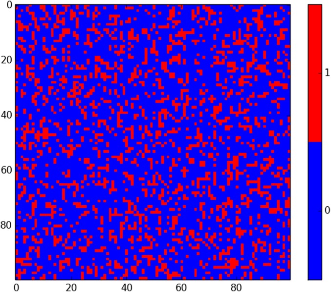
Table 1 gives the equilibrium frequencies of strategy 1 for various values of $\lambda$ and $w$. Note that the agreement with the limiting result is very good when $w=1/10$ and good when $w=1/2$. Fig. 1 gives the final configuration of the simulation when $\lambda =3$. Here and in later figures, we will quantify the spatial structure by computing the nearest-neighbor correlation

$${\rho }_{ij}=\frac{f_{ij}-f_i{f}_j}{{\sigma }_i{\sigma }_j},$$

where $f_{ij}$ is the fraction of nearest neighbor pairs with states $i$, and $j$, $f_i$ is the frequency of type $i$ and ${\sigma }_i=\sqrt{f_i(1-f_i)}$ is the SD.

Table 1.

Simulation results for the public goods game

$\lambda$	4/3	3/2	3	3.5	4
Original game	0.11	0.25	0.75	0.83	0.89
w = 1/2	0.01	0.19	0.79	0.88	0.96
w = 1/10	0.00	0.16	0.82	0.92	0.98
$\text{𝑤}\to \mathrm{𝟎}$ limit	0	0.17	0.83	0.93	1

Fig. 1.

Simulation of the original public goods game $G_1$ with $\lambda =3$. Here and in Figs. 4, 5, and 7, the picture gives the state of slice through a $100\times 100\times 100$ grid. Visually there is very little spatial structure in equilibrium. The correlation ${\rho }_{11}=0.006657$.

3. Three-Strategy Games

We will suppose that the game is written in the form

$$G=\begin{array}{cccc}& \hfill \mathrm{𝟏}\hfill & \hfill \mathrm{𝟐}\hfill & \hfill \mathrm{𝟑}\hfill \\ \hfill \mathrm{𝟏}\hfill & \hfill 0\hfill & \hfill {\alpha }_3\hfill & \hfill {\beta }_2\hfill \\ \hfill \mathrm{𝟐}\hfill & \hfill {\beta }_3\hfill & \hfill 0\hfill & \hfill {\alpha }_1\hfill \\ \hfill \mathrm{𝟑}\hfill & \hfill {\alpha }_2\hfill & \hfill {\beta }_1\hfill & \hfill 0\hfill \end{array}.$$ [6]

The subscripts indicate the strategy that has been left out in the various $2\times 2$ subgames.

In the $2\times 2$ case, there are only four possibilities: 1 dominates 2, 2 dominates 1, stable mixed strategy fixed point, and unstable mixed strategy fixed point. Bomze (15, 17) lists more than 40 possibilities for the $3\times 3$ case. Here, we do not consider games with unstable edge fixed points and only consider generic examples in which the six off-diagonal entries are nonzero and distinct, so we end up with 11 cases described in SI Appendix, Section S2. In the next three sections, we consider games with “rock–paper–scissors” relationships between the strategies and two examples in which the replicator equation has two locally attracting fixed points (bistability).

4. Rock–Paper–Scissors

Suppose that the ${\beta }_i>0$ and the ${\alpha }_i<0$ in Eq. 6. In this situation, there is an interior fixed point with all coordinates positive. Theorem 7.7.2 in Hofbauer and Sigmund (1) describes the asymptotic behavior of the replicator equations for these games.

Theorem 2.

Let $\mathrm{\Delta }={\beta }_1{\beta }_2{\beta }_3+{\alpha }_1{\alpha }_2{\alpha }_3$. If $\mathrm{\Delta }>0$, solutions converge to the fixed point (stable spiral). If $\mathrm{\Delta }<0$, their distance from the boundary tends to 0 (unstable spiral). If $\mathrm{\Delta }=0$, there is a one-parameter family of periodic orbits.

In ref. 3, the following result is proved, which covers some situations with stable spirals.

Theorem 3.

Suppose that the modified three-strategy game $H$ has (i) zeros on the diagonal, (ii) an interior equilibrium $\rho$, and that $H$ is almost constant sum: $H_{ij}+H_{ji}=\gamma +{\eta }_{ij}$ with $\gamma >0$ and ${\max }_{i,j}|{\eta }_{i,j}|<\gamma /2$. Then there is coexistence and furthermore for any $\delta >0$ if $\epsilon <{\epsilon }_0(\delta )$ and $\mu$ is any stationary distribution concentrating on configurations with infinitely many 1’s, 2’s, and 3’s we have

$$\underset{x}{sup}|\mu (\xi (x)=i)-{\rho }_i|<\delta .$$

In words, the equilibrium frequencies are close to those of the replicator equation for the modified game.

Turning to simulation, we first consider the constant sum game (which is covered by Theorem 3).

$$\begin{array}{cccc}\hfill G_2\hfill & \hfill \mathrm{𝟏}\hfill & \hfill \mathrm{𝟐}\hfill & \hfill \mathrm{𝟑}\hfill \\ \hfill \mathrm{𝟏}\hfill & \hfill 0\hfill & \hfill 4\hfill & \hfill -3\hfill \\ \hfill \mathrm{𝟐}\hfill & \hfill -1\hfill & \hfill 0\hfill & \hfill 5\hfill \\ \hfill \mathrm{𝟑}\hfill & \hfill 6\hfill & \hfill -2\hfill & \hfill 0\hfill \end{array}\begin{array}{cccc}\hfill H_2\hfill & \hfill \mathrm{𝟏}\hfill & \hfill \mathrm{𝟐}\hfill & \hfill \mathrm{𝟑}\hfill \\ \hfill \mathrm{𝟏}\hfill & \hfill 0\hfill & \hfill 6.5\hfill & \hfill -7.5\hfill \\ \hfill \mathrm{𝟐}\hfill & \hfill -3.5\hfill & \hfill 0\hfill & \hfill 8.5\hfill \\ \hfill \mathrm{𝟑}\hfill & \hfill 10.5\hfill & \hfill -5.5\hfill & \hfill 0\hfill \end{array}.$$

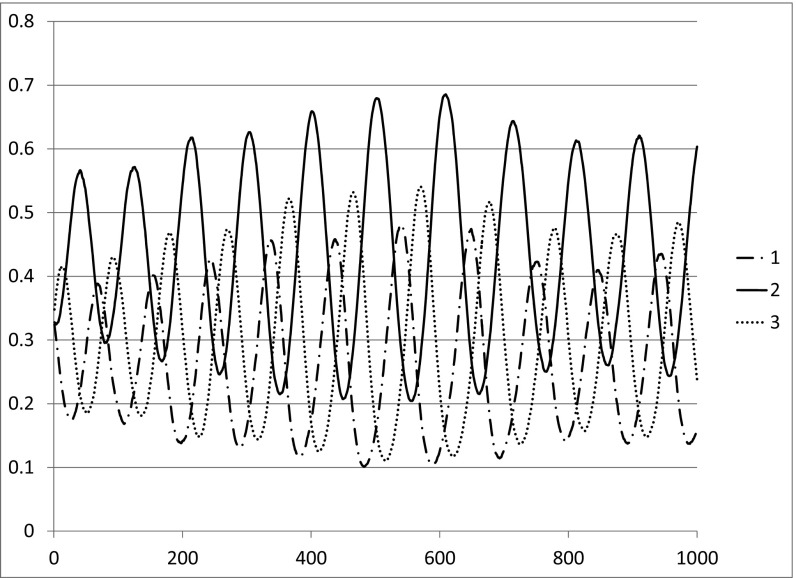
Note that $H_2$ is again constant sum. It has $\mathrm{\Delta }>0$, so the replicator equation spirals in to the fixed point, and Theorem 3 implies there is coexistence in the spatial game with weak selection. The simulation of the spatial game $1+0.2G$ given in Fig. 2 confirms this. Note that the observed densities of the three strategies are close to the theoretical prediction from the replicator equation for $H_2$. $(0.31,0.43,0.25)$.

Fig. 2.

Frequencies of the three strategies versus time in stable rock–paper–scissors game $1+0.2G_2$.

For our second example, we consider a game $G_3$ for which the modified game $H_3$ has $\mathrm{\Delta }<0$, and hence the solution to the replicator equation spirals out to the boundary.

$$\begin{array}{cccc}\hfill G_3\hfill & \hfill \mathrm{𝟏}\hfill & \hfill \mathrm{𝟐}\hfill & \hfill \mathrm{𝟑}\hfill \\ \hfill \mathrm{𝟏}\hfill & \hfill 0\hfill & \hfill 1\hfill & \hfill -2\hfill \\ \hfill \mathrm{𝟐}\hfill & \hfill -3\hfill & \hfill 0\hfill & \hfill 2\hfill \\ \hfill \mathrm{𝟑}\hfill & \hfill 3\hfill & \hfill -2\hfill & \hfill 0\hfill \end{array}\begin{array}{cccc}\hfill H_3\hfill & \hfill \mathrm{𝟏}\hfill & \hfill \mathrm{𝟐}\hfill & \hfill \mathrm{𝟑}\hfill \\ \hfill \mathrm{𝟏}\hfill & \hfill 0\hfill & \hfill 3\hfill & \hfill -4.5\hfill \\ \hfill \mathrm{𝟐}\hfill & \hfill -5\hfill & \hfill 0\hfill & \hfill 4\hfill \\ \hfill \mathrm{𝟑}\hfill & \hfill 5.5\hfill & \hfill -4\hfill & \hfill 0\hfill \end{array}.$$

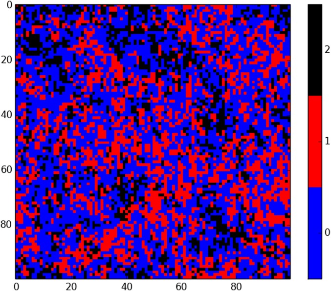
Fig. 3 shows that spatial structure stabilizes the unstable rock–paper–scissors example, i.e., the densities stay bounded away from 0. The apparent periodic behavior will disappear when a large enough system is simulated. For a discussion of this, see section 5 of a 1998 paper by Durrett and Levin (18). As explained in SI Appendix, Section S3, sufficiently large means that the side of the cube is much larger than the correlation length. Fig. 4 shows a picture of the final state in the simulation run that produced Fig. 3.

Fig. 3.

Frequencies of the three strategies versus time in the unstable rock–paper–scissors game $1+0.2G_3$.

Fig. 4.

Final state in the simulation in Fig. 3. Note that there is significant spatial correlation in contrast to the simulation of the public goods game in Fig. 1. Here, ${\rho }_{11}=0.1775$, ${\rho }_{22}=0.2256$ and ${\rho }_{33}=0.2031$.

5. Stag Hunt

To prepare for the discussion of bistable $3\times 3$ games, we begin with a $2\times 2$ example.

$$\begin{array}{ccc}& \hfill Stag\hfill & \hfill Hare\hfill \\ \hfill Stag\hfill & \hfill 4\hfill & \hfill 0\hfill \\ \hfill Hare\hfill & \hfill 2\hfill & \hfill 1\hfill \end{array}.$$

To explain the matrix: You can go hunt Stag (a large male deer), but if you go alone, then you have no chance to get one. If you hunt Hare and the other player hunts Stag, you get to keep all the rabbits. If you hunt Hare and the other player does also, then you split the kill.

If we transform so that there are 0’s on the diagonal and replace the strategy names by numbers, the game becomes $G$. The modified game is $H$.

$$\begin{array}{ccc}\hfill G\hfill & \hfill \mathrm{𝟏}\hfill & \hfill \mathrm{𝟐}\hfill \\ \hfill \mathrm{𝟏}\hfill & \hfill 0\hfill & \hfill -1\hfill \\ \hfill \mathrm{𝟐}\hfill & \hfill -2\hfill & \hfill 0\hfill \end{array}\hspace{1em}\hspace{1em}\hspace{1em}\begin{array}{ccc}\hfill H\hfill & \hfill \mathrm{𝟏}\hfill & \hfill \mathrm{𝟐}\hfill \\ \hfill \mathrm{𝟏}\hfill & \hfill 0\hfill & \hfill -0.5\hfill \\ \hfill \mathrm{𝟐}\hfill & \hfill -2.5\hfill & \hfill 0\hfill \end{array}.$$

In $H$, $({\rho }_1,{\rho }_2)=(1/6,5/6)$ is an unstable equilibrium. If $u_1>1/6$, the first strategy becomes more attractive and increases further.

It was shown in section 6 of ref. 3 that if ${\rho }_1<1/2$, then the 1’s take over the system. This is proved by considering the limiting PDE for the local density of strategy 1, which is

$$\frac{du}{dt}={\sigma }^2{u}^{″}/2+\varphi (u)\hspace{1em}\text{with}\hspace{1em}\varphi (u)=u(1-u)[b-(b+c)u],$$

where $b=-0.5$, $c=-2.5$. When $b,c<0$, this equation has a traveling wave solution that moves with velocity $v$

$$u(t,x)=w(x-vt),\hspace{1em}u(-\mathrm{\infty })=1,\hspace{1em}u(\mathrm{\infty })=0.$$

The 1’s take over if and only if $v>0$, which is equivalent to ${\int }_0^1\varphi (x)dx>0$. Since $\varphi$ is a cubic with zeros at 0 and 1, this holds if and only if the interior equilibrium $\rho =b/(b+c)<1/2$.

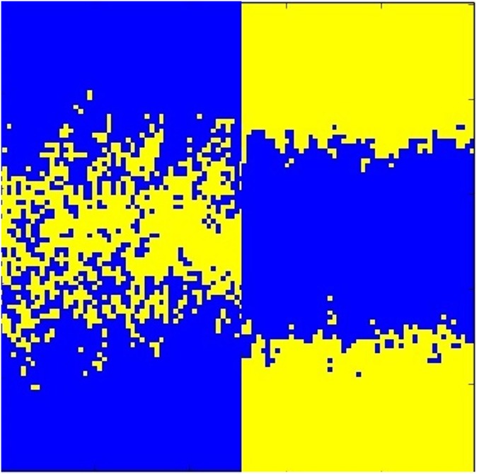
Fig. 5 gives a visual explanation of the difference between interfaces in the public goods and stag hunt games. For an explanation of the relevance of the behavior of interfaces to properties of stochastic spatial models, see the 1999 paper by Molofsky et al. (19).

Fig. 5.

The simulations were started with a strip of one strategy in between two strips of the opposite type. In the public goods game, on the left the interface melts down, and we have coexistence. In the Stag Hunt, on the right, the interface stays tight.

6. Multiple Myeloma

The original matrix, which we will call $G_4$, is given in Eq. 3. The modified game has entries

$$\begin{array}{cccc}\hfill H_4\hfill & \hfill \mathrm{𝟏}\hfill & \hfill \mathrm{𝟐}\hfill & \hfill \mathrm{𝟑}\hfill \\ \hfill \mathrm{𝟏}\hfill & \hfill 0\hfill & \hfill A\hfill & \hfill B\hfill \\ \hfill \mathrm{𝟐}\hfill & \hfill E\hfill & \hfill 0\hfill & \hfill -D\hfill \\ \hfill \mathrm{𝟑}\hfill & \hfill C\hfill & \hfill F\hfill & \hfill 0\hfill \end{array},$$

where $A=(1+\theta )a-\theta e$, $E=(1+\theta )e-\theta a$ $B=(1+\theta )b-\theta c$, $C=(1+\theta )c-\theta b$ $D=(1+\theta )d$, and $F=\theta d$. The modification of the game does not change the sign of $D$, but it puts a positive entry $F$ in $G_{\mathrm{3,2}}$. It may also change the signs of one or two of the other four nonzero entries. Noting that $A<0$ if $e>(1+\theta )a/\theta$ while $E<0$ if $e<\theta a/(1+\theta )$, we see that if one of these two entries is negative, the other one is positive. The same holds for $B$ and $C$, so there are nine possibilities for the signs of $A,B,C,E$ and a wide variety of possible behaviors for the spatial game that are not found in the replicator equation. In particular it is possible for all three strategies to coexist in the spatial model, but not in the replicator equation. These possibilities were systematically considered in section 9.1 of ref. 3. The dramatic differences between the properties of the spatial game and the replicator equation cast doubt on the proposed insights into therapy that emerge from the analysis of Dingli et al. (see the discussion that begins on page 1,134 of ref. 5).

Here, our interest in this model is as an example with bistability. Suppose that $A,B,C,E>0$ and $DC/BE>F/A$, which holds for the original game entries. Results from ref. 3, which are described in SI Appendix, Section S4, show that there are three cases:

Case 1.

$C/E>1-F/A$. The replicator equation converges to the 1,3 equilibrium.

Case 2.

$1-F/A>C/E>1-DC/BE$. There is an interior fixed point that is a saddle point, and the replicator equation exhibits bistability.

Case 3.

$1-DC/BE>C/E$. The replicator equation converges to the 1,2 equilibrium.

In our simulation of case 2 we take $a=e=2$, $d=1$, and vary $b=c$. The perturbed game is very simple in this case: $A=E=a=e$, $B=C=b=c$, $D=1.5$, $F=0.5$. Since $B=C=c$ the condition for case 2 is

$$1-\frac{0.5}{2}>\frac{c}{2}>1-\frac{1.5}{2},$$

or $1.5>c>0.5$. When $c=1.5$, the 1,3 equilibrium wins. When $c=1$, the 1,2 equilibrium wins. In principle we could find the value of $c$ where the limiting equilibrium changes by showing that the limiting system of PDE has traveling wave solutions and finding the parameter value where the velocity changes sign, but this seems to be difficult mathematical problem.

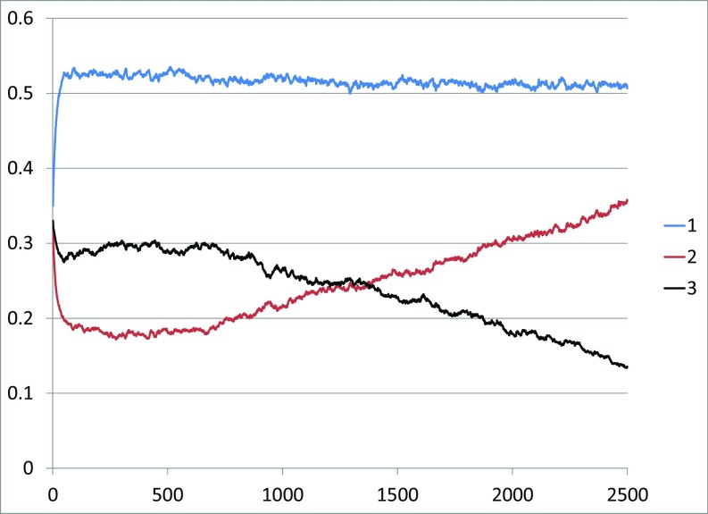
When $c=1.25$, the 1,2 equilibrium wins (Fig. 6), but takes a long time to do so, suggesting that this value is near the point where the limiting state changes. Fig. 7, which shows the final state of the simulation, shows that we get separation into regions that look like the two possible equilibria, and then the 1,2 regions grow and take over.

Fig. 6.

Frequencies versus time in a $100\times 100\times 100$ simulation of the weak selection multiple myeloma game $1+(1/3)G_4$, with $a=e=2$, $d=1$, and $b=c=1.25$. Note that the frequencies first get close to the unstable fixed point at $(0.531,0.306,0.1633)$ and then start heading toward the boundary equilibrium.

Fig. 7.

Picture of final configuration for the simulation in Fig. 6. Note that the blues (1’s) are spread throughout the space, while the reds (2’s) and whites (3’s) are segregated. The correlations ${\rho }_{11}=0.1342$, ${\rho }_{22}=0.1600$, and ${\rho }_{33}=0.1497$ are smaller than those in Fig. 4.

7. Summary

In this paper, we have used simulation and heuristic arguments to make predictions about the behavior of games that cannot be analyzed rigorously using the methods of ref. 3. The main contribution is to describe a procedure for determining the behavior of spatial three-strategy games with weak selection, when the game matrix $G$ has no unstable edge fixed points. One first forms the modified game $H_{ij}=(1+\theta )G_{ij}-\theta G_{j,i}$, where $\theta$ is a constant that depends on the spatial structure, but not on the entries in the game matrix. $\theta \approx 1/2$ in the three-dimensional nearest-neighbor case. The behavior of the spatial game with matrix $G$ can then be predicted from that of the replicator equation for $H$. We say predicted because in some cases the behavior is not the same.

For three-strategy games without unstable edge fixed points, there are four major types:

• 1.When there are 1, 2, or 3 stable edge fixed points and they can all be invaded, there is coexistence in the spatial evolutionary game when selection is small. This was proved in ref. 3
• 2.As first observed by Durrett and Levin (20), when the replicator equation is bistable, i.e., the limit depends on the starting point, the spatial game has a stronger equilibrium that is the limit for generic initial conditions. In two strategy games, the victorious strategy is determined by the direction of movement of the traveling wave solution of the PDE. For three-strategy games, we do not know how to prove the existence of such traveling waves or compute their speeds, but simulations suggest that the same result holds.
• 3.In the case of rock–paper–scissors games, there is coexistence when the replicator equation converges to the interior fixed point. This was proved in ref. 3 when the game is “almost constant sum.” It is somewhat surprising that when the replicator equation trajectories that spiral out to the boundary, space exerts a stabilizing effect and the three strategies coexist. This result has also been found recently by Ryser and Murgas (10).
• 4.Last, and least interesting, is the situation in which the replicator equation converges to a boundary fixed point. Simulations show (SI Appendix, Section S5) that the same behavior occurs in the spatial evolutionary game.

Work remains to be done on three-strategy games with unstable boundary fixed points; however, the work presented here can be used to analyze all of the games in all the papers we have cited except for one example in ref. 10. In many cases the behavior of the spatial game differs from that of the replicator equation, so it is important to consider the impact of spatial structure in order to obtain correct conclusions. The results we have presented here are derived in the limit that the selection $w\to 0$, but simulations show that in many cases the conclusions are accurate when $w=0.1$ or even 0.25.

References

- 1.Hofbauer J, Sigmund K. Evolutionary Games and Population Dynamics. Cambridge Univ Press; Cambridge, UK: 1998. [Google Scholar]
- 2.Cox T, Durrett R, Perkins E. 2011. Voter model perturbations and reaction diffusion equations. Astérisque 340. arXiv:1103.1676.
- 3.Durrett R. Spatial evolutionary games with small selection coefficients. Electron J Probab. 2014;19:121. [Google Scholar]
- 4.Archetti M, Ferraro DA, Christofori G. Heterogeneity for IGF-II production maintained by public goods dynamics in neuroendocrine pancreatic cancer. Proc Natl Acad Sci USA. 2015;112:1833–1838. doi: 10.1073/pnas.1414653112. [DOI] [PMC free article] [PubMed] [Google Scholar]
- 5.Dingli D, Chalub FACC, Santos FC, van Segbroeck S, Pacheco JM. Cancer phenotype as the outcome of an evolutionary game between normal and malignant cells. Br J Cancer. 2009;101:1130–1136. doi: 10.1038/sj.bjc.6605288. [DOI] [PMC free article] [PubMed] [Google Scholar]
- 6.Tomlinson IPM, Bodmer WF. Modeling the consequences of interactions between tumor cells. Br J Cancer. 1997;78:157–160. doi: 10.1038/bjc.1997.26. [DOI] [PMC free article] [PubMed] [Google Scholar]
- 7.Basanta D, Simon M, Hatzikirou H, Deutsch A. Evolutionary game theory elucidates the role of glycolysis in glioma progression and invasion. Cell Prolif. 2008;41:980–987. doi: 10.1111/j.1365-2184.2008.00563.x. [DOI] [PMC free article] [PubMed] [Google Scholar]
- 8.Basanta D, et al. Investigating prostate cancer tumor-stroma interactions: Clinical and biological insights from an evolutionary game. Br J Cancer. 2012;106:174–181. doi: 10.1038/bjc.2011.517. [DOI] [PMC free article] [PubMed] [Google Scholar]
- 9.Swierniak A, Krzeslak M. Application of evolutionary games to modeling carcinogenesis. Math Biosci Eng. 2013;10:873–911. doi: 10.3934/mbe.2013.10.873. [DOI] [PubMed] [Google Scholar]
- 10.Ryser R, Murgas KA. Bone remodeling as a spatial evolutionary game. J Thoer Biol. 2017;418:16–26. doi: 10.1016/j.jtbi.2017.01.021. [DOI] [PMC free article] [PubMed] [Google Scholar]
- 11.Bozic I, et al. Accumulation of driver and passenger mutations during tumor progression. Proc Natl Acad Sci USA. 2010;107:18545–18550. doi: 10.1073/pnas.1010978107. [DOI] [PMC free article] [PubMed] [Google Scholar]
- 12.Ohtsuki H, Nowak MA. Evolutionary games on graphs. J Theor Biol. 2006;243:86–97. doi: 10.1016/j.jtbi.2006.06.004. [DOI] [PMC free article] [PubMed] [Google Scholar]
- 13.Tarnita CE, Ohtsuki H, Antal T, Feng F, Nowak MA. Strategy selection in structured populations. J Theor Biol. 2009;259:570–581. doi: 10.1016/j.jtbi.2009.03.035. [DOI] [PMC free article] [PubMed] [Google Scholar]
- 14.Tarnita CE, Wage N, Nowak MA. Multiple strategies in structured populations. Proc Natl Acad Sci USA. 2011;108:2334–2337. doi: 10.1073/pnas.1016008108. [DOI] [PMC free article] [PubMed] [Google Scholar]
- 15.Bomze IM. Lotka-Volterra equation and replicator dynamics. Biol Cybern. 1983;48:201–211. [Google Scholar]
- 16.Durrett R, Levin SA. Stohastic spatial models: A user’s guide to ecological applications. Phil Trans R Soc London. 1994;343:329–350. [Google Scholar]
- 17.Bomze IM. Lotka-Volterra equation and replicator dynamics: New issues in the classification. Biol Cybern. 1983;72:447–453. [Google Scholar]
- 18.Durrett R, Levin SA. Spatial aspects of interspecific competition. Theor Popul Biol. 1998;53:30–43. doi: 10.1006/tpbi.1997.1338. [DOI] [PubMed] [Google Scholar]
- 19.Molofsky J, et al. Local frequency dependence and global coexistence. Theor Popul Biol. 1998;55:270–282. doi: 10.1006/tpbi.1998.1404. [DOI] [PubMed] [Google Scholar]
- 20.Durrett R, Levin SA. The importance of being discrete (and spatial) Theor Popul Biol. 1994;46:363–394. [Google Scholar]
Associated Data
This section collects any data citations, data availability statements, or supplementary materials included in this article.