Lotka-Volterra pairwise modeling fails to capture diverse pairwise microbial interactions

Abstract

Pairwise models are commonly used to describe many-species communities. In these models, an individual receives additive fitness effects from pairwise interactions with each species in the community ('additivity assumption'). All pairwise interactions are typically represented by a single equation where parameters reflect signs and strengths of fitness effects ('universality assumption'). Here, we show that a single equation fails to qualitatively capture diverse pairwise microbial interactions. We build mechanistic reference models for two microbial species engaging in commonly-found chemical-mediated interactions, and attempt to derive pairwise models. Different equations are appropriate depending on whether a mediator is consumable or reusable, whether an interaction is mediated by one or more mediators, and sometimes even on quantitative details of the community (e.g. relative fitness of the two species, initial conditions). Our results, combined with potential violation of the additivity assumption in many-species communities, suggest that pairwise modeling will often fail to predict microbial dynamics.

DOI: http://dx.doi.org/10.7554/eLife.25051.001

eLife digest

From the soil to our body, microbes, such as bacteria, are everywhere and affect us in many ways. Many microbes perform important roles in natural environments and for our health, but some of them can cause harm and lead to diseases. Often, microbes affect and interact with each other within large groups or communities. Because of their widespread ramifications, it is important to understand how microbial communities work.

In addition to experiments, mathematical modeling offers one way to gain insight into the dynamics of microbial communities. A model commonly used to describe the interactions between organisms is the so-called ‘pairwise model’. Pairwise models can be useful to predict the dynamics of a community in which two species physically interact, such as a predator-prey community. However, it was unknown if this model was suitable to adequately predict the dynamics of microbial species in communities. Microbes often interact via chemicals that diffuse in the environment. For example, one microbe might provide food for another microbe or release toxins to kill it. However, a pairwise model does not consider food or toxins, but only how one microbe stimulates or inhibits the growth of another.

Momeni et al. simulated different scenarios commonly found in microbial communities to test whether a pairwise model could capture how, for example, chemicals released by one bacterial species would either help others to grow or stop them from growing. The results showed that for many scenarios, pairwise models cannot qualitatively represent the dynamics of a microbial community.

A next step will be to work on the limitations of current experimental technologies and mathematical models to improve the understanding of microbial communities. This knowledge could be used to develop new strategies for ecosystem engineering, such as for example making soils more fertile to improve crop yields, or tackling antibiotic resistance of bacteria.

DOI: http://dx.doi.org/10.7554/eLife.25051.002

Introduction

Multispecies microbial communities are ubiquitous. Microbial communities are important for industrial applications such as cheese and wine fermentation (van Hijum et al., 2013) and municipal waste treatment (Seghezzo et al., 1998). Microbial communities are also important for human health: they can modulate immune responses and food digestion (Round and Mazmanian, 2009; Kau et al., 2011) during health and disease. Properties of the entire community (‘community properties’, e.g. species dynamics, ability to survive internal or external perturbations, and biochemical activities of the entire community) are influenced by interactions wherein individuals alter the physiology of other individuals (Widder et al., 2016). To understand and predict community properties, choosing the appropriate mathematical model to describe species interactions is critical.

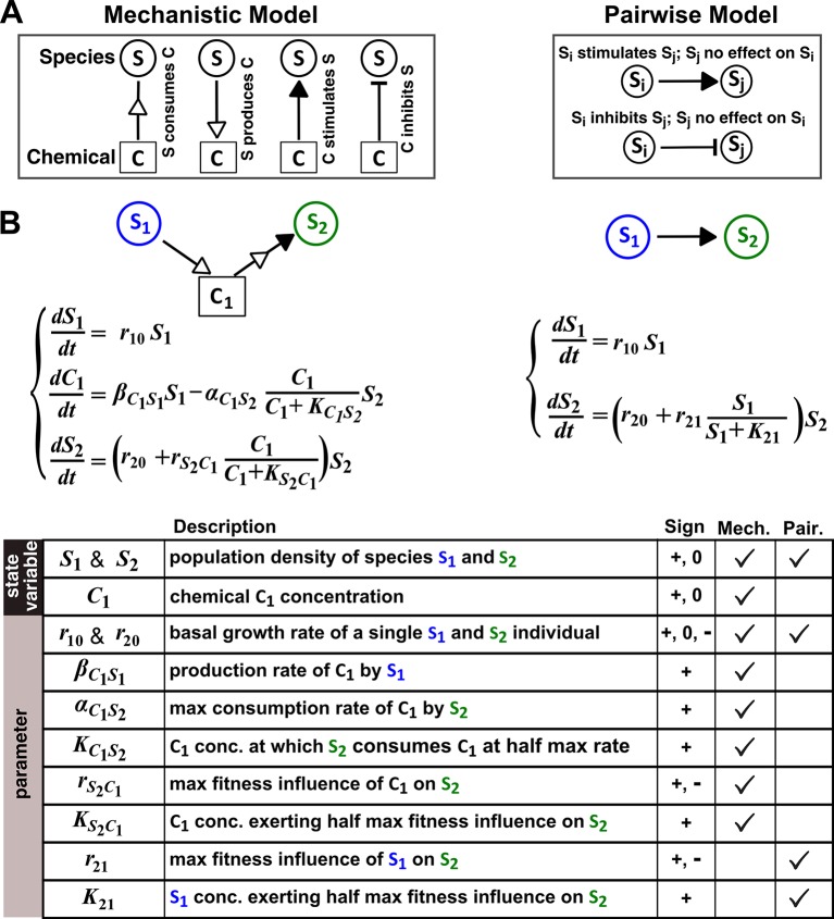
A mathematical model ideally focuses only on details that are essential to community properties of interest. However, it is often unclear a priori what the minimal essential details are. We define ‘mechanistic models’ as models that explicitly consider interaction mediators as state variables. For example, if species S₁ releases a compound C₁ which stimulates species S₂ growth upon consumption by S₂, then a mechanistic model tracks concentrations of S₁, C₁, and S₂ (Figure 1A and B, left panels). Note that mechanistic models used here still omit molecular details such as how chemical mediators are received and processed by recipients and how mediators subsequently act on recipients. In contrast, Lotka-Volterra (‘L-V’) pairwise models only consider the fitness effects of interactions. Specifically, L-V models assume that the fitness of an individual is the sum of its basal fitness (the net growth rate of an individual in isolation) and fitness influences from pairwise interactions with individuals of the same species and of every other species in the community (‘additivity’ assumption). Furthermore, regardless of interaction mechanisms or quantitative details of a community, all fitness influences are typically expressed using a single equation form wherein parameters can vary to reflect the signs and magnitudes of fitness influences (‘universality’ assumption). Thus in the example above, a pairwise model only describes how S₁ increases the fitness of S₂ (Figure 1A and B, right panels).

Figure 1. The abstraction of interaction mechanisms in a pairwise model compared to a mechanistic model.

(A) The mechanistic model (left) considers a bipartite network of species and chemical interaction mediators. A species can produce or consume chemicals (open arrowheads pointing towards and away from the chemical, respectively). A chemical mediator can positively or negatively influence the fitness of its target species (filled arrowhead and bar, respectively). The corresponding L-V pairwise model (right) includes only the fitness effects of species interactions, which can be positive (filled arrowhead), negative (bar), or zero (line terminus). (B) In the example here, species S₁ releases chemical C₁, and C₁ is consumed by species S₂ and promotes S₂’s fitness. In the mechanistic model, the three equations respectively state that (1) S₁ grows exponentially at a rate ${\displaystyle r_{10}}$, (2) C₁ is released by S₁ at a rate ${\beta }_{C_1{S}_1}$ and consumed by S₂ with saturable kinetics (maximal consumption rate ${\alpha }_{C_1{S}_2}$ and half-saturation constant $K_{C_1{S}_2}$), and (3) S₂’s growth (basal fitness ${\displaystyle r_{20}}$) is influenced by C₁ in a saturable fashion. In the pairwise model here, the first equation is identical to that of the mechanistic model. The second equation is similar to the last equation of the mechanistic model except that ${\displaystyle r_{21}}$ and ${\displaystyle K_{21}}$ together reflect how the density of S₁ (${\displaystyle S_1}$) affects the fitness of S₂ in a saturable fashion. For all parameters with double subscripts, the first subscript denotes the focal species or chemical, and the second subscript denotes the influencer. Note that unlike in mechanistic models, we have omitted ‘${\displaystyle S}$’ from subscripts in pairwise models (e.g. ${\displaystyle r_{21}}$ instead of $r_{S_2{S}_1}$) for simplicity. In this example, both ${\displaystyle r_{21}}$ and $r_{S_2{S}_1}$ are positive.

DOI: http://dx.doi.org/10.7554/eLife.25051.003

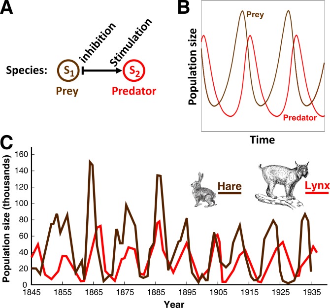
Figure 1—figure supplement 1. An L-V pairwise model successfully predicts oscillations in population dynamics of the hare-lynx prey-predator community.

(A) In a pairwise model of prey-predation proposed by Lotka and Volterra, predator reduces the fitness of prey, while prey stimulates the fitness of predator. Such dynamics can be easily simulated (Green and Shou, 2014). (B) Assuming random encounter between prey and predator, the pairwise model predicts oscillations in the prey and predator population sizes. (C) Similar oscillations have been qualitatively observed in natural populations of lynx (predator) and hare (prey), providing support for the usefulness of pairwise models. Picture is adapted from https://biologyeoc.wikispaces.com/PopulationChanges (BiologyEOC, 2016).

DOI: http://dx.doi.org/10.7554/eLife.25051.004

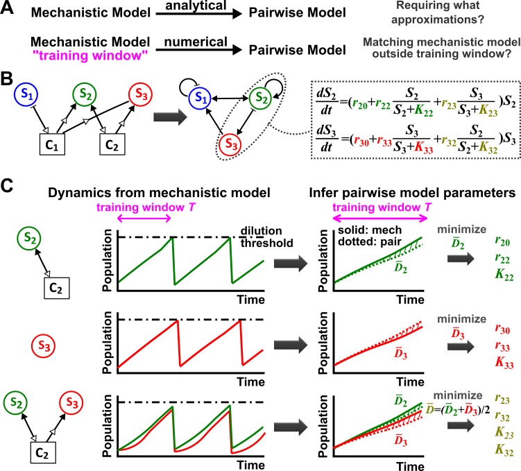
Figure 1—figure supplement 2. Deriving a pairwise model.

(A) Analytically deriving a pairwise model from a mechanistic model allows us to uncover approximations required for such a transformation (top). Alternatively (bottom), within a ‘training window’ of the mechanistic model population dynamics, we can numerically derive parameters for a pre-selected pairwise model such that it best fits the mechanistic model. We then quantify how well such a pairwise model matches the mechanistic model under conditions different from those of the training window. (B) A mechanistic model of three species interacting via two chemicals (left) can be translated into a pairwise model of three interacting species (center). S₁ inhibits S₁ and promotes S₂ (via C₁). S₂ promotes S₂ and S₃ (via C₂) as well as S₁ (via removal of C₁). S₃ promotes S₁ (via removal of C₁) and inhibits S₂ (via removal of C₂). Take interactions between S₂ and S₃ for example: the saturable L-V pairwise model will require estimating ten parameters (colored, right), some of which (e.g. ${\displaystyle r_{33}}$ in this case) may be zero. (C) In the numerical method, the six monoculture parameters (${\displaystyle r_{i0}}$, ${\displaystyle r_{ii}}$, and ${\displaystyle K_{ii}}$, ${\displaystyle i}$ = 2, 3; green and red) are first estimated from training window ${\displaystyle T}$ (within a dilution cycle) of monoculture mechanistic models (top and middle). Subsequently, the four interaction parameters ( and ${\displaystyle K_{ij}}$, , olive) can be estimated from the training window ${\displaystyle T}$ of the S₂ +S₃ coculture mechanistic model (bottom). Parameter definitions are described in Figure 1. Often in this work, pairwise model parameters that can be directly obtained from the mechanistic model (e.g. species basal fitness; ) are directly obtained from the mechanistic model (instead of being estimated). To estimate parameters, we use an optimization routine to minimize $\overline{D}$, the fold-difference (hatched area) between dynamics from a pairwise model (dotted lines) and the mechanistic model (solid lines) averaged over ${\displaystyle T}$ and species number ${\displaystyle N}$: ${\displaystyle \overline{D}=\frac{1}{N}\sum _{i=1}^N\left[\frac{1}{T}{\int }_T{D}_i\left(t\right)dt\right]=\frac{1}{N}\sum _{i=1}^N\left[\frac{1}{T}{\int }_T|lo{g}_{10}\left(S_{i,pair}\left(t\right)/S_{i,mech}\left(t\right)\right)|dt\right]}$. Here ${\displaystyle S_{i,pair}}$ and ${\displaystyle S_{i,mech}}$ are ${\displaystyle S_i}$ calculated using pairwise and mechanistic models, respectively. Since species with densities below a set extinction limit, ${\displaystyle S_{ext}}$, are assumed to have gone extinct in the model, we set all densities below the extinction limit to ${\displaystyle S_{ext}}$ in calculating $\overline{D}$ to avoid singularities. $\overline{D}$ outside the training window can be used to quantify how well the best-matching pairwise model predicts the mechanistic model. Unless otherwise stated, in all simulations to ensure that resources not involved in interactions are never limiting, a community is diluted back to its inoculation density whenever total population increases to a high-density threshold, mimicking turbidostat experiments. Too frequent dilutions will allow only small changes in population dynamics within a dilution cycle or time ${\displaystyle T}$, which is not suitable for estimating pairwise model parameters. Dilutions can sometimes violate conditions for convergence to reference dynamics (Figure 3—figure supplement 4). Under most cases we have tested, small variations in dilution frequency do not affect our conclusions. See Methods-Summary of simulation files for relevant Matlab codes.

DOI: http://dx.doi.org/10.7554/eLife.25051.005

L-V pairwise models are popular. L-V pairwise modeling has successfully explained the oscillatory dynamics of hare and its predator lynx (Figure 1—figure supplement 1) (Volterra, 1926; Wangersky, 1978; BiologyEOC, 2016). Pairwise models have also been instrumental in delineating conditions for multiple carnivores to coexist when competing for herbivores (MacArthur, 1970; Chesson, 1990). In both cases, mechanistic models and pairwise models happen to be mathematically equivalent for the following reasons. In the hare-lynx example, both species are also interaction mediators, and therefore pairwise and mechanistic models are identical. In the second example, if herbivores (mediators of competitive interactions between carnivores) rapidly reach steady state, herbivores can be mathematically eliminated from the mechanistic model to yield a pairwise model of competing carnivores (MacArthur, 1970; Chesson, 1990). Pairwise models are often used to predict how perturbations to steady-state species composition exacerbate or decline over time (May, 1972; Thébault and Fontaine, 2010; Mougi and Kondoh, 2012; Allesina and Tang, 2012; Suweis et al., 2013; Coyte et al., 2015). Although most work are motivated by contact-dependent prey-predation (e.g. hare-lynx) or mutualisms (e.g. plant-pollinator) where L-V models could be identical to mechanistic models, these work do not explicitly exclude chemical-mediated interactions where species are distinct from interaction mediators.

The temptation of using pairwise models is indeed high, including in microbial communities where many interactions are mediated by chemicals (Mounier et al., 2008; Faust and Raes, 2012; Stein et al., 2013; Marino et al., 2014; Coyte et al., 2015). Even though pairwise models do not capture the dynamics of chemical mediators, predicting species dynamics is still highly desirable in, for example, forecasting species diversity and compositional stability. For chemical-mediated interactions, L-V pairwise models are far easier to construct than mechanistic models for the following reasons. Mechanistic models would require knowledge of chemical mediators, which are often challenging to identify. Since chemical mediators are explicitly modeled, mechanistic models require more equations and parameters than their cognate pairwise models (Figure 1, Table). Pairwise model parameters are relatively easy to estimate using community dynamics or dynamics of monocultures and pairwise cocultures (Mounier et al., 2008; Stein et al., 2013; Guo and Boedicker, 2016). Consequently, pairwise modeling has been liberally applied to microbial communities.

L-V pairwise models have been criticized when applied to communities of more than two species (referred to as ‘multispecies communities’) (Levine, 1976; Tilman, 1987; Wootton, 1993, 2002; Werner and Peacor, 2003; Stanton, 2003; Schmitz et al., 2004). This is because a third species can influence interactions between a species pair (‘indirect interactions’), which sometimes violates the additivity assumption of pairwise models. For example, a carnivore can indirectly increase the density of a plant by decreasing the density of an herbivore (‘interaction chain’; ‘density-mediated indirect interactions’). A carnivore can also decrease how often an herbivore forages plants (‘interaction modification’, ‘trait-mediated indirect interactions’, or ‘higher order interactions’) (Vandermeer, 1969; Wootton, 1994; Billick and Case, 1994; Wootton, 2002). In interaction modification, foraging per herbivore decreases, whereas in interaction chain, the density of herbivores decreases. Interaction modification (but not interaction chain) violates the additivity assumption (Methods-Interaction modification but not interaction chain violates the additivity assumption) (Tilman, 1987; Wootton, 1994; Schmitz et al., 2004) and can cause the pairwise model to generate qualitatively wrong predictions. Indeed, pairwise models largely failed to predict biomass and species coexistence in three-species and seven-species plant communities (Dormann and Roxburgh, 2005), although reported failures of pairwise models could be due to limitations in data collection and analysis (Case and Bender, 1981; Billick and Case, 1994).

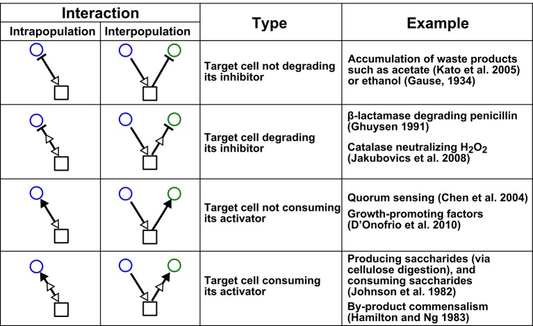
Here, we examine the universality assumption of pairwise models when applied to microbial communities (or any community that employs diverse chemical-mediated interactions). Microbes often influence other microbes in a myriad of fashions, via consumable metabolites, reusable signaling molecules, or a combination of chemicals (Figure 2). Can a single equation form, traditionally employed in pairwise models, qualitatively describe diverse interactions between two microbial species? The answer is unclear. On the one hand, pairwise models have been applied successfully to diverse microbial communities. For example, an L-V pairwise model and a mechanistic model both correctly predicted ratio stabilization and spatial intermixing between two strongly-cooperating populations exchanging diffusible essential metabolites (Momeni et al., 2013). In other examples, pairwise models largely captured competition outcomes and metabolic activities of three-species and four-species artificial microbial communities (Vandermeer, 1969; Guo and Boedicker, 2016; Friedman et al., 2017). On the other hand, pairwise models often failed to predict species coexistence in seven-species microbial communities (Friedman et al., 2017), although this could be due to interaction modification discussed above.

Figure 2. Chemical-mediated interactions commonly found in microbial communities.

Interactions can be intra- or inter-population. Examples are meant to be illustrative instead of comprehensive.

DOI: http://dx.doi.org/10.7554/eLife.25051.006

Instead of investigating natural communities where interaction mechanisms can be difficult to identify, we use in silico communities. In these communities, two species interact via mechanisms commonly encountered in microbial communities, including growth-promoting and growth-inhibiting interactions mediated by reusable and consumable compounds (Figure 2) (Stams, 1994; Czárán et al., 2002; Duan et al., 2009). We construct mechanistic models for these two-species communities and attempt to derive from them pairwise models. A mechanistic reference model offers several advantages: community dynamics is deterministically known; deriving a pairwise model is not limited by inaccuracy of experimental methods; and the flexibility in creating different reference models allows us to explore a variety of interaction mechanisms. We demonstrate that a single pairwise equation form often fails for commonly-encountered diverse pairwise microbial interactions. We conclude by discussing when pairwise models might or might not be useful, in light of our findings.

Results

Throughout this work, we consider communities grown in a well-mixed environment where all individuals interact with each other with an equal chance. A well-mixed environment can be found in industrial fermenters. Moreover, at a sufficiently small spatial scale, a spatially-structured environment can be approximated as a well-mixed environment, as chemicals are uniformly-distributed locally. Motile organisms also reduce the degree of spatial structure. A well-mixed environment allows us to use ordinary differential equations (ODEs), which are more tractable than partial differential equations demanded by a spatially-structured environment. This in turn allows us to sometimes analytically demonstrate failures of pairwise models.

Mechanistic model versus pairwise model

A mechanistic model describes how species release or consume chemicals and how chemicals stimulate or inhibit species growth (Figure 1A left). In contrast, in pairwise models, interation mediators are not explicitly considered (Figure 1A right). Instead, the growth rate of an individual of species S_i is the sum of its basal fitness (${\displaystyle r_{i0}}$, net growth rate of the individual in the absence of any intra-species or inter-species interactions) and fitness effects from intra-species and inter-species interactions. The fitness effect from species S_j to species S_i is represented by $f_{ij}\left(S_j\right)$, where ${\displaystyle S_j}$ is the density of species S_j. $f_{ij}\left(S_j\right)$ is a linear or nonlinear function of only ${\displaystyle S_j}$ and not of another species. When ${\displaystyle j=i}$, ${\displaystyle f_{ii}\left(S_i\right)}$ represents density-dependent fitness effect within S_i (e.g. density-dependent growth inhibition or stimulation).

In a multi-species pairwise model, a single form of $f_{ij}$ is used for all pairwise species interactions. For example, the most popular L-V model is linear L-V:

$$\frac{d{S}_i}{dt}=\left[r_{i0}+{\displaystyle \sum _j{r}_{ij}{S}_j}\right]S_i$$ (1)

Here, $r_{i0}$ is the basal fitness of an individual of S_i, and can be positive, negative, or zero; $r_{ij}$ is the fitness effect per S_j individual on S_i. Positive, negative, or zero $r_{ij}$ represents growth stimulation, inhibition, or no effect, respectively. An example of linear L-V is the logistic L-V pairwise model traditionally used for competitive communities:

$$\frac{d{S}_i}{dt}=r_{i0}\left[1-{\displaystyle \sum _j\frac{S_j}{{\Lambda }_{ij}}}\right]S_i$$ (2)

Here, nonnegative $r_{i0}$ is the basal fitness of S_i; positive ${\Lambda }_{ij}$ is the carrying capacity imposed by limiting shared resource (e.g. space or carbon source) such that a single S_i individual will have a zero net growth rate when competing with a total of ${\Lambda }_{ij}$ individuals of S_j.

Alternative forms of fitness effect $f_{ij}$ (Wangersky, 1978) include L-V with delayed influence, where the fitness influence of one species on another may lag in time (Gopalsamy, 1992), or saturable L-V (Thébault and Fontaine, 2010) where

$$\frac{d{S}_i}{dt}=\left[r_{i0}+{\displaystyle \sum _j{r}_{ij}\frac{S_j}{K_{ij}+S_j}}\right]S_i$$ (3)

Here, $r_{i0}$ is the basal fitness of an individual of S_i, $r_{ij}$ is the maximal fitness effect species S_j can exert on S_i, and ${\displaystyle K_{ij}}$ (>0) is the ${\displaystyle S_j}$ at which half maximal fitness effect on S_i is achieved. $r_{i0}$ and $r_{ij}$ can be positive, negative, or zero. Note that at a low concentration of influencer, the saturable form can be converted to a linear form.

Our goal is to test whether a single equation form of pairwise model can qualitatively predict dynamics of species pairs engaging in various types of interactions commonly found in microbial communities (e.g. Figure 2). To do so, we use a combination of analytical and numerical approaches (Figure 1—figure supplement 2). Analytically deriving a pairwise model from a mechanistic model not only reveals assumptions required to generate the pairwise model, but also alleviates any concern that we may have failed to identify the optimal pairwise model parameters. When interactions become more complex (e.g. involving multiple mediators), we take the numerical approach, which is typically used to infer pairwise models from experimental results (Pascual and Kareiva, 1996). In the numerical approach, we mimic experimentalists by first deciding on a pairwise model to be used, and then employing a nonlinear least squares routine to numerically identify model parameters that minimize the average difference $\overline{D}$ between pairwise and mechanistic model dynamics within a training time window ${\displaystyle T}$ (Figure 1—figure supplement 2; Methods-Summary of simulation files). To evaluate how well a pairwise model predicts long-term mechanistic model dynamics, we ‘buy time’ by introducing 'dilutions' in numerical simulations of both models and quantify their difference $\overline{D}$.

Reusable versus consumable mediators require different pairwise models

In this section, we analytically derive pairwise models from mechanistic models of two-species communities where one species affects the other species through a single mediator. The mediator is either reusable such as signaling molecules in quorum sensing (Duan et al., 2009; Jakubovics, 2010) or consumable such as metabolites (Stams, 1994; Freilich et al., 2011) (Figure 2). We show that a single pairwise model may not encompass these different interaction mechanisms and that for consumable mediator, the choice of pairwise model also depends on details such as the relative fitness and initial densities of the two species.

Consider a commensal community where species S₁ stimulates the growth of species S₂ by producing a reusable (Figure 3A) or a consumable (Figure 3B) chemical C₁. We consider community dynamics where species are not limited by any abiotic resources, such as within a dilution cycle of a turbidostat experiment where all other metabolites are in excess.

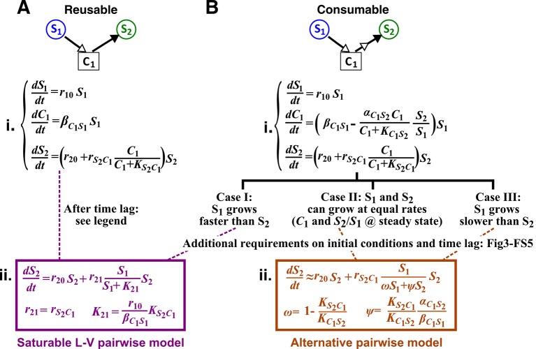
Figure 3. Interactions mediated via a single mediator are best represented by different forms of pairwise models, depending on whether the mediator is consumable or reusable and on the relative fitness and initial densities of the two species.

S₁ stimulates the growth of S₂ via a reusable (A) or a consumable (B) chemical C₁. In mechanistic models of the two cases (i), equations for ${\displaystyle S_1}$ and ${\displaystyle S_2}$ are identical but equations for ${\displaystyle C_1}$ are different. In (A), ${\displaystyle C_1}$ can be solved to yield ${\displaystyle C_1=\left({\beta }_{C_1{S}_1}/r_{10}\right)S_{10}\exp \left(r_{10}t\right)-\left({\beta }_{C_1{S}_1}/r_{10}\right)S_{10}=\left({\beta }_{C_1{S}_1}/r_{10}\right)S_1-\left({\beta }_{C_1{S}_1}/r_{10}\right)S_{10}}$, assuming zero initial ${\displaystyle C_1}$. Here, ${\displaystyle S_{10}}$ is ${\displaystyle S_1}$ at time zero. We have approximated ${\displaystyle C_1}$ by omitting the second term (valid after the initial transient response has passed so that ${\displaystyle C_1}$ has become proportional to ${\displaystyle S_1}$). This approximation allows an exact match between the mechanistic model and the saturable L-V pairwise model (ii). In (B), depending on the relative growth rates of the two species, and if additional requirements are satisfied (Methods; Figure 3—figure supplement 2; Figure 3—figure supplement 3; Figure 3—figure supplement 4; Figure 3—figure supplement 5), either saturable L-V or alternative pairwise model should be used.

DOI: http://dx.doi.org/10.7554/eLife.25051.007

Figure 3—figure supplement 1. For a reusable mediator, parameter estimation after acclimation time leads to a more accurate saturable L-V pairwise model.

(A) We use the mechanistic model for a reusable mediator to generate reference dynamics of , , and over 150 generations of community growth. Note that population fractions (instead of population densities) are plotted, which fluctuate less than the mediator concentration during dilutions. After an initial period of time, becomes proportional to (inset). The basal fitness of S₁ and S₂ in pairwise models are identical to those in mechanistic models, and here and (= 1, 2) are irrelevant due to the lack of intra-population interactions. We use every 10 community doublings (within a dilution cycle) of reference dynamics as training windows to numerically estimate best-matching saturable L-V pairwise model parameters and . Dashed and solid rectangles represent a training window before and after acclimation, respectively. (B) Pairwise model parameters estimated after acclimation (e.g. solid rectangle) match their analytically-derived counterparts (black dotted lines) better than those estimated before acclimation (e.g. dashed rectangle). (C) A pairwise model generated from population dynamics before acclimation (top) predicts future reference dynamics less accurately than that generated after acclimation (bottom). (D) Quantification of the difference between pairwise and mechanistic models before (dashed) or after (solid) acclimation. All parameters are listed in Figure 3—source data 1.

DOI: http://dx.doi.org/10.7554/eLife.25051.012

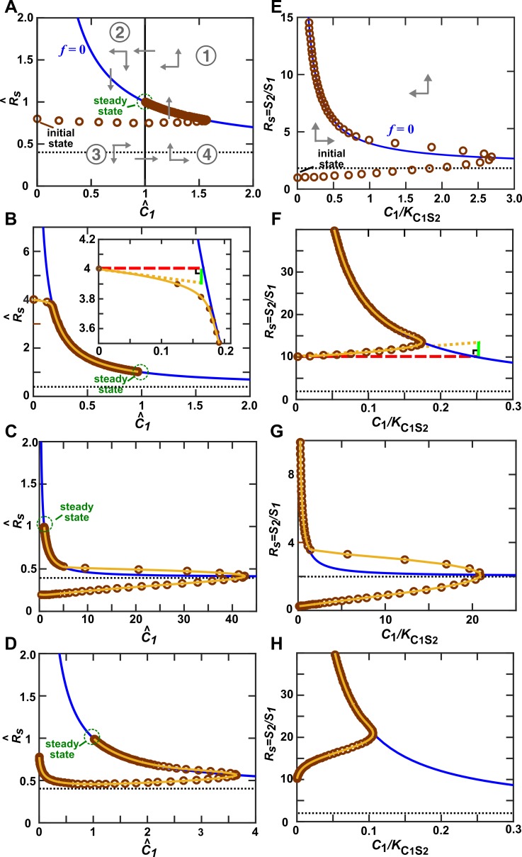
Figure 3—figure supplement 2. Community trajectory approaching the -zero-isocline allows us to use the alternative pairwise model approximation.

S₁ releases a consumable metabolite C₁ which stimulates S₂ growth. In all panels, brown circles indicate the ${\displaystyle C_1}$ and ${\displaystyle R_S}$ (${\displaystyle =S_2/S_1}$) of a community, and are separated by 1/4 of community doubling time. In the vicinity of the ${\displaystyle f}$-zero-isocline ($f=0$) (blue line), can be eliminated to yield a pairwise model. (A–D) When $r_{S_2{C}_1}>r_{10}-r_{20}>0$ (Methods-Deriving a pairwise model for interactions mediated by a single consumable mediator, Case II), a steady state (green circle) exists. Let us scale and against their respective steady state values to obtain ${\displaystyle {\hat{R}}_S}$ and ${\displaystyle {\hat{C}}_1}$. The ${\displaystyle f}$-zero-isocline (blue) and the steady state ${\displaystyle {\hat{C}}_1=1}$ (vertical solid line) divide the phase portrait into four regions (① to ④). (A) The directions of movement are marked by grey arrowheads. According to the top portion of Equation 11,the right-hand side of Equation 14 is zero when ${\displaystyle {\hat{C}}_1=1}$. Since ${\displaystyle {\hat{C}}_1/\left({\hat{C}}_1+{\hat{K}}_{S_2{C}_1}\right)=1/\left(1+{\hat{K}}_{S_2{C}_1}/{\hat{C}}_1\right)}$ is an increasing function of ${\displaystyle {\hat{C}}_1}$, when ${\displaystyle {\hat{C}}_1>1}$, ${\displaystyle d{\hat{R}}_S/dt}$ > 0 (up arrows), and when ${\displaystyle {\hat{C}}_1}$<1, ${\displaystyle d{\hat{R}}_S/dt}$<0 (down arrows). From Equation 15, above the ${\displaystyle f}$-zero-isocline, ${\displaystyle d{\hat{C}}_1/dt}$<0 (left arrows), while below the ${\displaystyle f}$-zero-isocline, ${\displaystyle d{\hat{C}}_1/dt}$>0 (right arrows). Thus, the community moves toward the ${\displaystyle f}$-zero-isocline, and then moves slowly alongside (but not superimposing) the ${\displaystyle f}$-zero-isocline before reaching the steady state. A–C respectively describe community dynamics trajectories from when $S_{10}$ is large and when ${\displaystyle {\hat{R}}_S\left(t=0\right)\approx 1}$ (Case II-2), ${\displaystyle {\hat{R}}_S\left(t=0\right)\gg max(1,{\hat{K}}_{S_2{C}_1}^{-1})}$ (Case II-1), or ${\displaystyle {\hat{R}}_S\left(t=0\right)\ll 1/\left(1+{\hat{K}}_{C_1{S}_2}\right)}$ (Case II-3). (D) ${\displaystyle {\hat{R}}_S\left(t=0\right)\approx 1}$ but $S_{10}$ is much smaller than that in A. In this case, instead of approaching the ${\displaystyle f}$-zero-isocline quickly as in A, the trajectory plunges sharply before moving toward the ${\displaystyle f}$-zero-isocline. The black dotted line marks ${\displaystyle {\hat{R}}_S=1/\left(1+{\hat{K}}_{C_1{S}_2}\right)}$, the asymptotic value of ${\displaystyle f}$-zero-isocline. (E–H) When $r_{10}-r_{20}<0$ (Methods-Deriving a pairwise model for interactions mediated by a single consumable mediator, Case III), there is no steady state. ${\displaystyle R_S}$ approaches infinity and ${\displaystyle C_1}$ approaches 0. The black dotted line marks $R_S={\beta }_{C_1{S}_1}/{\alpha }_{C_1{S}_2}$, the asymptotic value of ${\displaystyle f}$-zero-isocline. E, F, and G respectively describe community dynamics trajectories from ${\displaystyle C_1=0}$ when $S_{10}$ is large and when $R_S\left(0\right)\approx {\beta }_{C_1{S}_1}/{\alpha }_{C_1{S}_2}$, $R_S\left(0\right)\gg {\beta }_{C_1{S}_1}/{\alpha }_{C_1{S}_2}$ (Case III-1), and $R_S\left(0\right)\ll {\beta }_{C_1{S}_1}/{\alpha }_{C_1{S}_2}$ (Case III-2). (H) $R_S\left(0\right)\gg {\beta }_{C_1{S}_1}/{\alpha }_{C_1{S}_2}$ but $S_{10}$ is much smaller than that in F. Note different axis scales in different figure panels. All parameters are listed in Figure 3—source data 2.

DOI: http://dx.doi.org/10.7554/eLife.25051.013

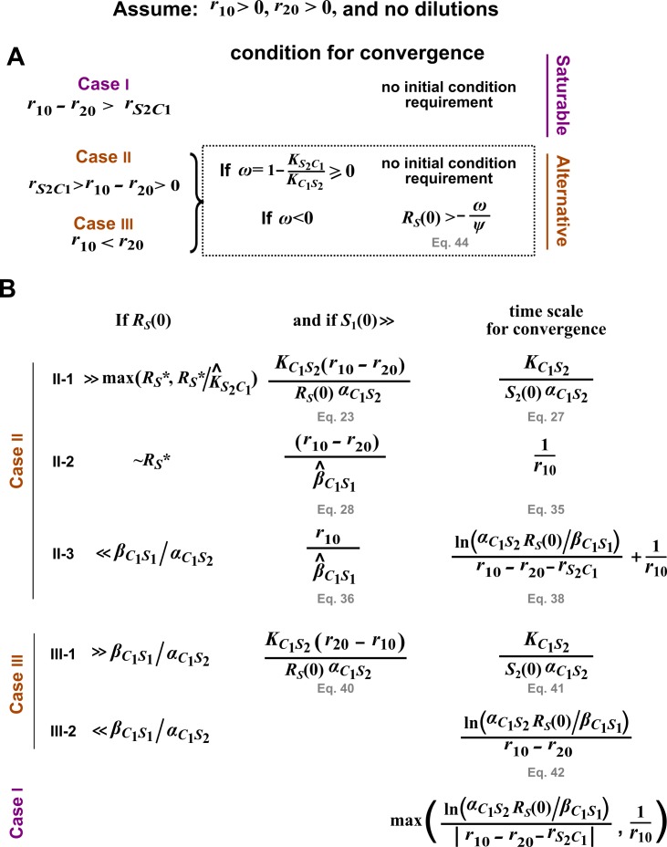
Figure 3—figure supplement 3. Condition for the alternative pairwise model to converge to the mechanistic model in the absence of dilutions.

Here are the phase portraits of Equation 43. The olive vertical dotted lines correspond to $R_S=-\omega /\psi$, a singularity point when $\omega <0$. (A) Case II ($r_{S_2{C}_1}>r_{10}-r_{20}>0$), $\omega =0.5$, $\psi =0.25$. Regardless of initial , the solution converges to steady state (in agreement with the mechanistic model). (B) Case II, $\omega =-1$, $\psi =1$. When $R_S(t=0)<-\omega /\psi$ (to the left of olive line), the alternative pairwise model falsely predicts extinction of S₂. (C) Case III ($r_{10}<r_{20}$), $\omega =0.8$, $\psi =0.1$. Regardless of initial , the model predicts extinction of S₁ (in agreement with the mechanistic model). (D) Case III ($r_{10}<r_{20}$), $\omega =-9$, $\psi =5$. When $R_S(t=0)<-\omega /\psi$ (to the left of olive line), the alternative pairwise model falsely predicts steady state coexistence of the two species. All parameters are listed in Figure 3—source data 3.

DOI: http://dx.doi.org/10.7554/eLife.25051.014

Figure 3—figure supplement 4. Initial conditions that require long convergence time and thus dilutions may prevent the alternative pairwise model to converge to the mechanistic model.

We consider commensalism through a consumable mediator, where the producer and the consumer could reach a steady state (Methods-Deriving a pairwise model for interactions mediated by a single consumable mediator, Case II). We choose a low consumption rate such that starting from equal proportions of producers and consumers, consumption can be neglected. (A) When the initial total population density is low (2 × 10⁵ total cells/ml, and periodic 10x dilution maintains this low density), the community cannot approach the blue -zero-isocline in a reasonable time frame (brown trajectory in the phase space of ${\displaystyle {\hat{C}}_1}$ and ${\displaystyle {\hat{R}}_S}$, the mediator concentration and the consumer-to-producer ratio normalized to their potential steady state values, respectively). As a result, growth and dilution lead to an alternate sustained cycle for the community (inset). (B) In this case, accumulates proportionally to within each dilution cycle, and the ratio of to reaches a constant value (inset). (C) Since behaves as a reusable mediator and since the community remains far from the -zero-isocline, the use of the alternative pairwise model (dashed) is not justified. Instead, the saturable L-V pairwise model (dotted) provides a better approximation. (D) The same community at a higher initial total density (2 × 10⁸ total cells/ml) approaches the blue -zero-isocline (brown trajectory in the phase space) after a few dilutions. (E) In the vicinity of the -zero-isocline, reaches its steady state value within each dilution cycle. (F) In this case, the alternative model produces a better approximation to the mechanistic model compared to a saturable L-V model. In (C) and (F), the saturable L-V model is fitted into dynamics of the reference model after 50 generations, whereas analytical formulas are used for the alternative pairwise model. All parameters are listed in Figure 3—source data 4.

DOI: http://dx.doi.org/10.7554/eLife.25051.015

Figure 3—figure supplement 5. Additional requirements for deriving a pairwise model from a mechanistic model, when S₁ affects S₂ via a single consumable mediator C₁ where ${\displaystyle C_1(0)=0}$.

For details, see Methods. Here, $R_S=S_2/S_1$. ${\displaystyle S_1(0)}$, ${\displaystyle S_2(0)}$, $C_1\left(0\right)$, and $R_S\left(0\right)$ are the initial values of the respective variables. (A) The initial condition requirement for a pairwise model to converge to the mechanistic model. (B) The time scale required for convergence. Conditions on ${\displaystyle S_1(0)}$ are sufficient, but may not be necessary.

DOI: http://dx.doi.org/10.7554/eLife.25051.016

When C₁ is reusable, the mechanistic model (Figure 3A,i) can be transformed into a saturable L-V pairwise model (compare Figure 3A,ii with Equation 3), especially after the concentration of the mediator (which is initially zero) has acclimated to be proportional to the producer population size (Figure 3A legend; Figure 3—figure supplement 1). This saturable L-V pairwise model is valid regardless of whether the producer coexists with the consumer, outcompetes the consumer, or is outcompeted by the consumer.

If C₁ is consumable, different scenarios are possible (Figure 3B; Methods).

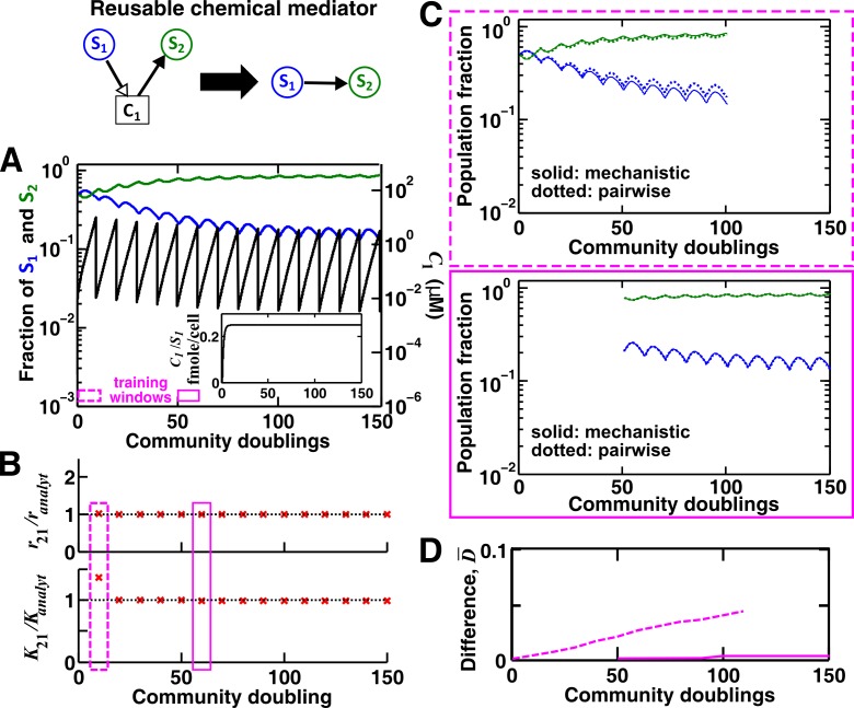
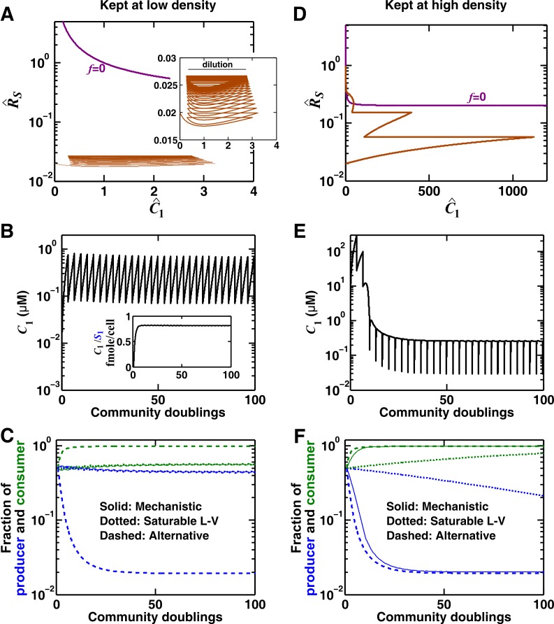
Case I: When supplier S₁ always grows faster than consumer S₂ (the basal fitness of S₁ is higher than the maximal fitness of S₂), ${\displaystyle C_1}$ will eventually accumulate proportionally to ${\displaystyle S_1}$ (Figure 4A left; Methods-Deriving a pairwise model for interactions mediated by a single consumable mediator Case I). In this case, C₁ may be approximated as a reusable mediator and can be predicted by the saturable L-V pairwise model (Figure 4A right, compare dotted and solid lines).

Figure 4. Saturable L-V and alternative pairwise models are not interchangeable.

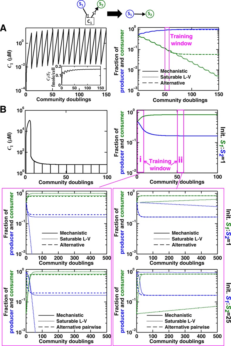
Consider a commensal community with a consumable mediator C₁. (A) The mediator accumulates without reaching a steady state within each dilution cycle as the consumer S₂ gradually goes extinct (Figure 3B, Case I). After a few tens of generations, $C_1$ becomes proportional to its producer density ${\displaystyle S_1}$ (inset in left panel). In this case, a saturable L-V (dotted) but not the alternative pairwise model (dashed) is suitable. All parameters are listed in Figure 4—source data 1. (B) The consumable mediator reaches a non-zero steady state within each dilution cycle (Figure 3B, Case II). From mechanistic dynamics where initial species ratio is 1, we use two training windows to derive saturable L-V (dotted) and alternative (dashed) pairwise models. We then use these pairwise models to predict dynamics of communities starting at two different ratios. The alternative model but not the saturable L-V predicts the mechanistic model dynamics. All parameters are listed in Figure 4—source data 2. Note that in all figures, population fractions (instead of population densities) are plotted, which fluctuate less during dilutions compared to mediator concentration.

DOI: http://dx.doi.org/10.7554/eLife.25051.017

Case II: When S₁ and S₂ can coexist (the basal fitness of S₁ is higher than the basal fitness of S₂ but less than the maximal fitness of S₂), a steady state solution for $C_1$ and species ratio $R_S=S_2/S_1$ exists (Figure 4B; Methods-Deriving a pairwise model for interactions mediated by a single consumable mediator Case II, Equation 11). To arrive at a pairwise model, we will need to eliminate $C_1$ which is mathematically possible (i.e. after community dynamics converges to the ‘${\displaystyle f}$-zero-isocline’ on the phase plane of mediator $C_1$ and species ratio ${\displaystyle R_S}$, as depicted by blue lines in Figure 3—figure supplement 2A–D). However, the derived pairwise model differs from the saturable L-V model:

$${\displaystyle \frac{d{S}_2}{dt}=r_{20}{S}_2+\frac{r_{S_2{C}_1}{S}_1}{\omega S_1+\psi S_2}{S}_2}$$ (4)

where constants $r_{20}$, $r_{S_2{C}_1}$, and ${\displaystyle \omega =1-K_{S_2{C}_1}/K_{C_1{S}_2}}$ can be positive, negative, or zero, and ψ =$\left(K_{S_2{C}_1}{\alpha }_{C_1{S}_2}\right)/\left(K_{C_1{S}_2}{\beta }_{C_1{S}_1}\right)$ is positive (see Figure 1 table for parameter definitions and see Equation 13 in Methods). We will refer to this equation as ‘alternative pairwise model’, although the fitness influence term is a function of both ${\displaystyle S_1}$ and ${\displaystyle S_2}$ instead of the influencer ${\displaystyle S_1}$ alone as defined in the traditional L-V pairwise model.

Case III: When supplier S₁ always grows slower than consumer S₂, i.e. when the basal fitness of S₁ (${\displaystyle r_{10}}$) is less than the basal fitness of S₂ (${\displaystyle r_{20}}$), consumable ${\displaystyle C_1}$ declines to zero concentration. This is because C₁ is consumed by S₂ whose relative abundance over S₁ eventually exponentially increases at a rate of $r_{20}-r_{10}$. Similar to Case II, under certain conditions (i.e. after community dynamics converges to the ${\displaystyle f}$-zero-isocline as seen in Figure 3—figure supplement 2E–H), the alternative pairwise model (Equation 4) can be derived (Methods-Deriving a pairwise model for interactions mediated by a single consumable mediator, Case III).

For both Case II and Case III, we analytically demonstrate that in the absence of dilutions, alternative pairwise model dynamics can converge to mechanistic model dynamics (see Figure 3—figure supplements 3 and 5 for initial condition requirement and time scale of convergence). However, if initial ${\displaystyle S_1}$ and ${\displaystyle S_2}$ are such that the time scale of convergence is long compared to the duration of one dilution cycle (e.g. Figure 3—figure supplement 2C and G), then we will have to perform dilutions and the saturable L-V model can sometimes be more appropriate than the alternative model (Figure 3—figure supplement 4). Thus in these cases, whether a saturable L-V or an alternative model is more appropriate also depends on initial conditions.

The alternative model (Equation 4) can be further simplified to

$$d{S}_2/dt=\left(r_{20}+\rho S_1/S_2\right)S_2$$ (5)

if additionally, the half-saturation constant ${\displaystyle K}$ for C₁ consumption ($K_{C_1{S}_2}$) is identical to that for C₁’s influence on the growth of consumer ($K_{S_2{C}_1}$), and if S₂ has not gone extinct. This equation form has precedence in the literature (e.g. [Mougi and Kondoh, 2012]), where the interaction strength ${\displaystyle r_{21}}$ reflects the fact that the consumable mediator from ${\displaystyle S_1}$ is divided among consumer ${\displaystyle S_2}$. Thus, we can regard the alternative model (Equation 4) or its simplified version (Equation 5) as a ‘divided influence’ model.

The saturable L-V model and the alternative model are not interchangeable (Figure 4). When a consumable mediator accumulates without reaching a steady state within each dilution cycle (Figure 4A left; inset: ${\displaystyle C_1}$ eventually becomes proportional to ${\displaystyle S_1}$), the saturable L-V model is predictive of community dynamics (Figure 4A right, compare dotted and solid lines). In contrast, predictions from the alternative pairwise model are qualitatively wrong (Figure 4A right, compare dashed and solid lines). When a consumable mediator eventually reaches a non-zero steady state within each dilution cycle (Figure 4B, black), could a saturable L-V model still work? The saturable L-V model derived from training window i (initial 10 generations) fails to predict species coexistence regardless of initial species ratios (Figure 4B left magenta box, compare solid with dotted). In comparison, the saturable L-V model derived from training window ii (at steady-state species ratio) performs better, especially if the starting species ratio is identical to that of the training dynamics (Figure 4B, top panel in right magenta box). However, at a different starting species ratio, the saturable L-V model fails to predict which species dominates the community (Figure 4B, bottom panel in right magenta box). In contrast, community dynamics can be described by the alternative pairwise model derived from either window i or ii (Figure 4B, compare dashed and solid lines in left and right magenta boxes).

We have shown here that even when one species affects another species via a single mediator, either a saturable L-V model or an alternative pairwise model may be appropriate. The appropriate model depends on whether the mediator is reusable or consumable, how fitness of the two species compare, and initial species densities (Figure 3; Figure 3—figure supplements 2–5). Choosing the wrong pairwise model generates qualitatively flawed predictions (Figure 4). Considering that reusable and consumable mediators are both common in microbial interactions, our results call for revisiting the universality assumption of pairwise modeling.

Two-mediator interactions require pairwise models different from single-mediator interactions

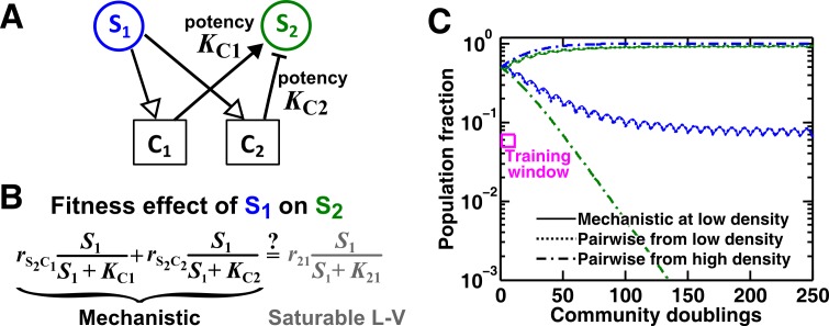
A species often affects another species via multiple mediators (Kato et al., 2008; Yang et al., 2009; Traxler et al., 2013; Kim et al., 2013). For example, a fraction of a population might die and release numerous chemicals, and some of these chemicals can simultaneously affect another individual. Here we examine the case where S₁ releases two reusable chemicals C₁ and C₂, both affecting the growth of S₂ (Figure 5A). Since the effect of each mediator can be described by a saturable L-V pairwise model (Figure 3A), we ask when the two mediators can be mathematically regarded as one mediator and described by a saturable L-V pairwise model (Figure 5B).

Figure 5. An example of a two-mediator interaction where a saturable L-V pairwise model may succeed or fail depending on initial conditions.

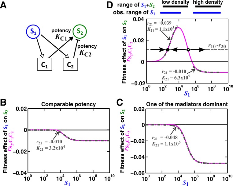
(A) One species can affect another species via two reusable mediators, each with a different potency ${\displaystyle K_{Ci}}$ where ${\displaystyle K_{Ci}}$ is $K_{S_2{C}_i}{r}_{10}/{\beta }_{C_i{S}_1}$ (Methods-Conditions under which a saturable L-V pairwise model can represent one species influencing another via two reusable mediators). A low ${\displaystyle K_{Ci}}$ indicates a strong potency (e.g. high release of C_i by S₁ or low ${\displaystyle C_i}$ required to achieve half-maximal influence on S₂). (B) Under what conditions can an interaction via two reusable mediators with saturable effects on recipients be approximated by a saturable L-V pairwise model? (C) A community where the success or failure of a saturable L-V pairwise model depends on initial conditions. Here, ${\displaystyle K_{C1}}$= 10³ cells/ml and ${\displaystyle K_{C2}}$= 10⁵ cells/ml. Community dynamics starting at low ${\displaystyle S_1}$ (solid) can be predicted if the saturable L-V pairwise model is derived from reference dynamics starting at low (dotted). However, if we use a saturable L-V pairwise model derived from a community with high initial ${\displaystyle S_1}$, prediction is qualitatively wrong (dash dot line). See Figure 5—figure supplement 1D for an explanation why a saturable L-V pairwise model estimated at one community density may not be applicable to another community density. Simulation parameters are listed in Figure 5—source data 1 .

DOI: http://dx.doi.org/10.7554/eLife.25051.020

Figure 5—figure supplement 1. Except under special conditions, a pairwise interaction through two mediators may not be represented by a single saturable L-V model.

(A) Consider the interaction in Figure 5. The fitness effect of S₁ on S₂ via C₁ and C₂ is $r_{S_2,C_1{C}_2}=\frac{r_{S_2{C}_1}{S}_1}{S_1+K_{S_2{C}_1}{r}_{10}/{\beta }_{C_1{S}_1}}+\frac{r_{S_2{C}_2}{S}_1}{S_1+K_{S_2{C}_2}{r}_{10}/{\beta }_{C_2{S}_1}}=\frac{r_{S_2{C}_1}{S}_1}{S_1+K_{C_1}}+\frac{r_{S_2{C}_2}{S}_1}{S_1+K_{C_2}}$. (B–C) Under special conditions the fitness effect $r_{S_2,C_1{C}_2}$ (magenta line) can be approximated using a single saturable L-V model (grey dash-dot line) at all densities. These special conditions include when the potencies of two mediators, K_C1 and K_C2, are similar (B) or the potency of one mediator is orders of magnitude stronger than the other (C). Otherwise, saturable L-V pairwise models derived from a low-density community and from a high-density community can have qualitatively different parameters (D). Let’s first consider the low-density case (left black and blue bars corresponding to low total density and therefore low , respectively). When $r_{S_2,C_1{C}_2}$ (magenta line) is above the (${\displaystyle r_{10}-r_{20}}$) line (grey dashed line), the fitness of S₂ ($r_{S_2,C_1{C}_2}+r_{20}$) will be higher than the fitness of S₁. Thus, even though S₁ grows at its basal fitness during a dilution cycle, S₁ fraction will decrease. Thus ${\displaystyle S_1}$ will decrease at the next dilution cycle when total density is reset to a pre-fixed level (arrow pointing towards lower ${\displaystyle S_1}$). In contrast, when $r_{S_2,C_1{C}_2}<r_{10}-r_{20}$, S₁ population fraction and ${\displaystyle S_1}$ will increase at the next dilution cycle (arrow pointing towards higher ${\displaystyle S_1}$). Thus, the dynamics will converge to a steady state ratio (filled dot). Interaction coefficient of a saturable L-V (grey dash-dot line) is estimated to be a positive value ( =+0.039). In contrast, in the high-density case (right black and blue bars), $r_{10}>r_{S_2,C_1{C}_2}+r_{20}$, and S₂ goes extinct. Interaction coefficient of a saturable L-V (grey dash-dot line) is estimated to be a negative value ( = −0.010). As a result, a saturable L-V pairwise model with parameters estimated at high densities cannot predict communities at low densities (Figure 5). All parameters are listed in Figure 5—source data 2.

DOI: http://dx.doi.org/10.7554/eLife.25051.023

We assume that fitness effects from different chemical mediators on a focal species are additive. Not making this assumption will likely violate the additivity assumption essential to pairwise models. Additive fitness effects have been observed for certain ‘homologous’ metabolites. For example, in multi-substrate carbon-limited chemostats of E. coli, the fitness effects from glucose and galactose were additive (Lendenmann and Egli, 1998). ‘Heterologous’ metabolites such as carbon and nitrogen sources likely affect cell fitness in a multiplicative fashion. However, if ${\displaystyle W_C}$ and ${\displaystyle W_N}$, the fitness influences of released carbon and nitrogen with respect to those already in the environment, are both small (i.e. ${\displaystyle W_C}$, ${\displaystyle W_N}$< < 1), the additional relative fitness influence will be additive: ${\displaystyle (1+W_C)(1+W_N)-1\approx W_C+W_N}$. However, we need to keep in mind that even among homologous metabolites, fitness effects may not be additive (Hermsen et al., 2015). ‘Sequential’ metabolites (e.g. diauxic shift) provide another example of non-additivity. Similar to the previous section, we assume that all abiotic resources are unlimited.

For the two reusable mediators, depending on their relative ‘potency’ (defined in Figure 5A legend), their combined effect generally cannot be modeled as a single mediator except under special conditions (Methods-Conditions under which a saturable L-V pairwise model can represent one species influencing another via two reusable mediators). These special conditions include: (1) mediators share similar potency (Figure 5—figure supplement 1B), or (2) one mediator dominates the interaction (Figure 5—figure supplement 1C). If these conditions are not satisfied, we can easily find examples where saturable L-V pairwise models derived from a low-density community and from a high-density community have qualitatively different parameters (Figure 5—figure supplement 1D). Consequently, the future dynamics of a low-density community can be predicted by a saturable L-V model derived from a low-density community but not by a model derived from a high-density community (Figure 5C). Thus, even though each mediator can be modeled by saturable L-V, their joint effects may or may not be modeled by saturable L-V depending on the relative potencies of the two mediators and sometimes even on initial conditions (high or low initial ${\displaystyle S_1}$).

Similarly, when both mediators are consumable and do not accumulate (as in Cases II and III of Figure 3B), the fitness effect term becomes $\frac{r_{S_2{C}_1}{S}_1}{{\omega }_{C_1}{S}_1+{\psi }_{C_1}{S}_2}+\frac{r_{S_2{C}_2}{S}_1}{{\omega }_{C_2}{S}_1+{\psi }_{C_2}{S}_2}$. Except under special conditions (e.g. when ${\omega }_{C_1}$ and ${\omega }_{C_2}$ are zero, or when ${\omega }_{C_1}/{\omega }_{C_2}={\psi }_{C_1}/{\psi }_{C_2}$, or when one mediator dominates the interaction), the two mediators may not be regarded as one. By the same token, when one mediator is a steady-state consumable and the other is reusable, they generally may not be regarded as a single mediator and would require yet a different pairwise model (i.e. with the fitness effect term $\frac{r_{S_2{C}_1}{S}_1}{{\omega }_{C_1}{S}_1+{\psi }_{C_1}{S}_2}+\frac{r_{S_2{C}_2}{S}_1}{S_1+K_{S_2{C}_2}{r}_{10}/{\beta }_{C_2{S}_1}}$).

In summary, when S₁ influences S₂ through multiple mediators, rarely can we approximate them as a single mediator. Sometimes, a pairwise model derived from one community may not apply to communities initiated at different densities (Figure 5C; Figure 5—figure supplement 1D). This casts further doubt on the usefulness of a single pairwise model for all pairwise microbial interactions.

L-V competition model can fail if two competing species engage in an additional interaction

So far, by assuming that abiotic resources are always present in excess (e.g. in turbidostats), we have not considered species competition for abiotic resources. In this section, we consider a competitive commensal community in a batch environment where S₁ and S₂ compete for an essential shared resource C₁ supplied by the environment at a constant rate (e.g. constant light), and S₁ supplies an essential consumable metabolite C₂ to promote S₂ growth (Figure 6A, left). We show that an L-V pairwise model works for some but not all communities even though these communities qualitatively share the same interaction mechanism.

Figure 6. An example of a competitive commensal community where an L-V pairwise model may work or fail.

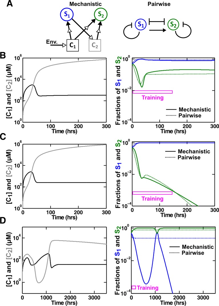
(A) Left: Two species S₁ and S₂ compete for shared resource C₁. Additionally, S₁ produces C₂ that promotes the growth of S₂ upon consumption. Right: An L-V pairwise model captures the intra- and inter-species competition as well as the commensal interaction between the two species. (B,C) Examples where L-V pairwise models predict the mechanistic reference dynamics well. (D) An example where the L-V pairwise model fails to predict the dynamics qualitatively (note the much longer time range). Here, population fractions fluctuate due to changes in relative concentration of C₁ compared to C₂. In all cases, the pairwise model is derived from the population dynamics in the initial stages of growth (150 hr in all cases). Simulation parameters are listed in Figure 6—source data 1.

DOI: http://dx.doi.org/10.7554/eLife.25051.024

In our mechanistic model (Methods-Competitive commensal interaction, Equation 47), the fitness of S₂ is multiplicatively affected by C₁ and C₂ (Mankad and Bungay, 1988). We choose parameters such that the effect from C₂ to S₂ is far from saturation (e.g. linear with respect to ${\displaystyle C_2}$ and ${\displaystyle S_1}$) to simplify the problem. In our L-V pairwise model (Figure 6A, right; Methods-Competitive commensal interaction, Equation 48), intra- and inter-species competition is represented by the traditional logistic L-V model (Equation 2; Gause, 1934; Thébault and Fontaine, 2010; Mougi and Kondoh, 2012). We then introduce a linear term (${\displaystyle r_{21}{S}_1}$) to describe the fitness effect of commensal interaction.

We tested various sets of mechanistic model parameters where the two species coexist in a steady fashion (Figure 6B), or one species goes extinct (Figure 6C), or species composition fluctuates (Figure 6D). L-V pairwise models deduced from a fixed period of training time could predict future dynamics in the first two cases, but failed to do so in the third case. Thus, depending on dynamic details of communities, a pairwise model sometimes works and sometimes fails.

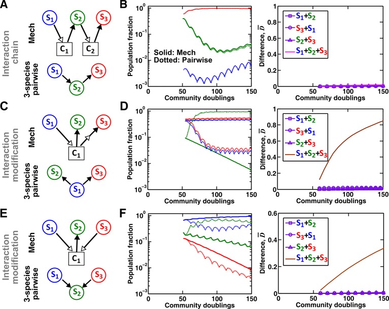
To summarize our work, even for pairwise microbial interactions, depending on interaction mechanisms (reusable versus consumable mediator, single mediator versus multiple mediators), we will need to use a plethora of pairwise models to avoid qualitative failures in predicting which species dominates a community or whether species coexist (Figures 3, 4 and 5). Sometimes, even when different communities share identical interaction mechanisms, depending on details such as relative species fitness, interaction strength, and initial conditions, the best-fitting pairwise model may or may not predict future dynamics (Figure 3B, Figure 3—figure supplement 4, Figure 4, Figure 5, Figure 5—figure supplement 1, and Figure 6). This defeats the very purpose of pairwise modeling – using a single equation form to capture fitness effects of all pairwise species interactions regardless of interaction mechanisms or quantitative details. In a community of more than two microbial species, interaction modification can cause pairwise models to fail (Figure 7). Even if species interact in an interaction chain and thus interaction modification does not occur, various chain segments may require different forms of pairwise models. Taken together, a pairwise model is unlikely to be effective for predicting community dynamics especially if interaction mechanisms are diverse.

Figure 7. Interaction chain but not interaction modification may be represented by a multispecies pairwise model.

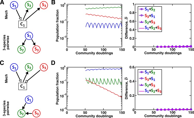
We examine three-species communities engaging in indirect interactions. Each species pair is representable by a two-species pairwise model (saturable L-V or alternative pairwise model, purple in the right columns of B, D, and F). We then use these two-species pairwise models to construct a three-species pairwise model, and test how well it predicts the dynamics known from the mechanistic model. In B, D, and F, left panels show dynamics from the mechanistic models (solid lines) and three-species pairwise models (dotted lines). Right panels show the difference metric $\overline{D}$. (A–B) Interaction chain: S₁ affects S₂, and S₂ affects S₃. The two interactions employ independent mediators C₁ and C₂, and both interactions can be represented by the saturable L-V pairwise model. The three-species pairwise model matches the mechanistic model in this case. Simulation parameters are provided in Figure 7—source data 1. (C–F) Interaction modification. In both cases, the three-species pairwise model fails to predict reference dynamics even though the dynamics of each species pair can be represented by a pairwise model. (C–D) S₃ consumes C₁, a mediator by which S₁ stimulates S₂. Parameters are listed in Figure 7—source data 2. Here, S₁ changes the nature of interaction between S₂ and S₃: S₂ and S₃ do not interact in the absence of S₁, but S₃ inhibits S₂ in the presence of S₁. The three-species pairwise model makes qualitatively wrong prediction about species coexistence. As expected, if S₃ does not remove C₁, the three-species pairwise model works (Figure 7—figure supplement 1A–B). (E–F) S₁ and S₃ both supply C₁ which stimulates S₂. Here, no species changes ‘the nature of interactions’ between any other two species: both S₁ and S₃ contribute reusable C₁ to stimulate S₂. S₁ promotes S₂ regardless of S₃; S₃ promotes S₂ regardless of S₁; S₁ and S₃ do not interact regardless of S₂. However, a multispecies pairwise model assumes that the fitness effects from the two producers on S₂ will be additive, whereas in reality, the fitness effect on S₂ saturates at high . As a result, the three-species pairwise model qualitatively fails to capture relative species abundance. As expected, if C₁ affects S₂ in a linear fashion, the community dynamics is accurately captured in the multispecies pairwise model (Figure 7—figure supplement 1C–D). Simulation parameters are listed in Figure 7—source data 3.

DOI: http://dx.doi.org/10.7554/eLife.25051.026

Figure 7—figure supplement 1. A multispecies pairwise model can work under special conditions.

(A–B) As a control for Figure 7C, if S₃ does not remove the mediator of interaction between S₁ and S₂, a three-species pairwise model accurately matches the mechanistic model. Simulation parameters are provided in Figure 7—source data 4. (C–D) As a control for Figure 7E, we ensured that fitness effects from multiple species are additive. In this case, a three-species pairwise model can represent the mechanistic model. To ensure the linearity and additivity of fitness effects, we have used a larger value of half saturation concentration ($K_{S_2{C}_1}$=10³ μM, instead of 10⁻¹ μM in Figure 7E–F). We have adjusted the interaction coefficients accordingly such that the overall interaction strength exerted by S₁ and S₃ on S₂ is comparable to that in Figure 7E–F (as evident by comparable population compositions). Since the interaction influences under these conditions remain in the linear range, the three-species pairwise model accurately predicts the reference dynamics. Simulation parameters are provided in Figure 7—source data 5.

DOI: http://dx.doi.org/10.7554/eLife.25051.032

Discussions

Multispecies pairwise models are widely used in theoretical ecology due to their simplicity. These models assume that all pairwise species interactions can be captured by a single pairwise model regardless of interaction mechanisms or quantitative details of a community (universality assumption). This assumption may be satisfied if, for example, interaction mediators are always species themselves (e.g. prey-predation in a food web) so that pairwise models are equivalent to mechanistic models. However, interactions in microbial communities are diverse and often mediated by chemicals (Figure 2). Here, we consider the validity of universality assumption of pairwise models in well-mixed, two-species microbial communities. We have focused on various types of chemical-mediated interactions commonly encountered in microbial communities (Figure 2) (Kato et al., 2005; Gause, 1934; Ghuysen, 1991; Jakubovics et al., 2008; Chen et al., 2004; D'Onofrio et al., 2010; Johnson et al., 1982; Hamilton and Ng, 1983). For each type of species interaction, we construct a mechanistic model to generate reference community dynamics (akin to experimental results). We then attempt to derive the best-matching pairwise model and ask how predictive it is.

We first consider cases where abiotic resources are in excess. When one species affects another species via a single chemical mediator, either the saturable L-V or the alternative pairwise model is appropriate, depending on the interaction mechanism (consumable versus reusable mediator), relative fitness of the two species, and initial conditions (Figure 3; Figure 3—figure supplement 2 to Figure 3—figure supplement 5). These two models are not interchangeable (Figure 4). If one species influences another species through multiple mediators, then in general, these mediators may not be regarded as a single mediator nor representable by a single pairwise model. For example, for two reusable mediators, unless their potencies are similar or one mediator is much more potent than the other, saturable L-V model parameters can qualitatively differ depending on initial community density (Figure 5—figure supplement 1D). Consequently, a pairwise model derived from a high-density community generates false predictions for low-density communities (Figure 5C), limiting the usefulness of pairwise models. We then consider a community where two species compete for a shared resource while engaging in commensalism via a single chemical mediator. We find that the best-fitting L-V pairwise model can predict future dynamics in some but not all communities, depending on parameters used in the mechanistic model (Figure 6). Thus, although a single equation form can work in many cases, it generates qualitatively wrong predictions in many other cases.

In communities of more than two microbial species, indirect interactions via a third species can occur. When indirect interactions take the form of interaction chains, if each chain segment of two species engages in an independent interaction and can be represented by a pairwise model, then multispecies pairwise models can work (Figure 7A-B). However, as discussed above, pairwise equation forms may vary among chain segments depending on interaction mechanisms and quantitative details of a community. When indirect interactions take the form of interaction modification, even if each species pair can be accurately represented by a pairwise model, a multispecies pairwise model may fail (Figure 7C–F, ). Interaction modification includes trait modification (Wootton, 2002; Werner and Peacor, 2003; Schmitz et al., 2004), or, in our cases, mediator modification. Mediator modification is very common in microbial communities. For example, antibiotic released by one species to inhibit another species may be inactivated by a third species, and this type of indirect interactions can stabilize microbial communities (Kelsic et al., 2015; Bairey et al., 2016). As another example, interaction mediators are often generated by and shared among multiple species. For example in oral biofilms, organic acids such as lactic acid are generated from carbohydrate fermentation by many species (Bradshaw et al., 1994; Marsh and Bradshaw, 1997; Kuramitsu et al., 2007). Such by-products are also consumed by multiple species (Kolenbrander, 2000).

One can argue that an extended pairwise model (e.g. $\frac{d{S}_2}{dt}=r_{20}{S}_2+\frac{r_{S_{2}C}{S}_1}{\varsigma +\omega S_1+\psi S_2}{S}_2$) embodying both the saturable form and the alternative form can serve as a general-purpose model at least for pairwise interactions via a single mediator. In fact, even the effects of indirect interactions may be quantified and included in the model by incorporating higher-order interaction terms (Case and Bender, 1981; Worthen and Moore, 1991), although with many challenges (Wootton, 2002). In the end, although these strategies may lead to a sufficiently accurate phenomenological model especially within the training window, they may fail to predict future dynamics.

When might a pairwise model be useful? First, pairwise models have been instrumental in understanding ecological phenomena such as prey-predator oscillatory dynamics and coexistence of competing predator species (Volterra, 1926; MacArthur, 1970; Case and Casten, 1979; Chesson, 1990). In these cases, mechanistic models are either identical to pairwise models or can be transformed into pairwise models under simplifying assumptions. Second, pairwise models of pairwise species interactions can provide a bird’s-eye view of strong or weak stimulatory or inhibitory interactions in a community. For example, Vetsigian et al., 2011 found that interactions between soil-isolated Streptomyces strains are enriched for reciprocity – if A inhibits or promotes B, it is likely that B also inhibits or promotes A (Vetsigian et al., 2011). Third, pairwise models have been useful in qualitatively understanding species assembly rules in small communities (Friedman et al., 2017). That is, qualitative information regarding species survival in competitions among a small number of species may be used to predict survival in more diverse communities within a similar time window. Fourth, a pairwise model can serve as a starting point for generating hypotheses on species interactions (e.g. Li et al., 2015). Note that when applied to microbial communities (Mounier et al., 2008; Stein et al., 2013; Marino et al., 2014), a fitting pairwise model means that the training dynamics of the community under investigation can be approximated by a theoretical community where species interactions satisfy the additivity and universality assumptions of pairwise models. Even though the theoretical community is likely different from the real community, hypothesis formulation can still be valuable. Finally, pairwise models can be useful in making predictions of limited scales. For example, Stein et al. used 2/3 of community dynamics data as a training set to derive a multispecies pairwise model, and in the best-case scenario, the model generated reasonable predictions on the remaining 1/3 of data (Stein et al., 2013). However, as we have shown, pairwise models can generate qualitatively wrong predictions (Figures 4–7), especially if interaction mechanisms are diverse such as in microbial communities. Not surprisingly, predicting qualitative consequences of species removal or addition using a pairwise model has encountered difficulties, especially in communities of more than three species (Mounier et al., 2008; Friedman et al., 2017).

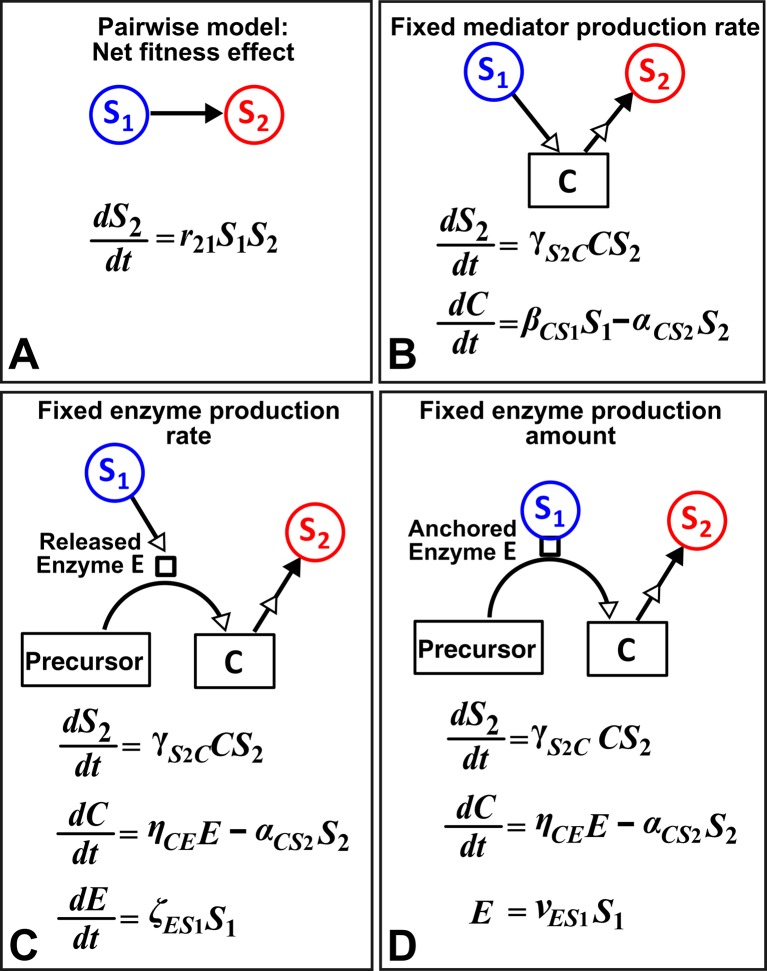
An alternative to a pairwise model is a mechanistic model. How much information about interaction mechanisms do we need to construct a mechanistic model? That is, what is the proper level of abstraction which captures the phenomena of interest, yet avoids unnecessary details (Li et al., 2015; Durrett and Levin, 1994)? For example, Tilman argued that if a small number of mechanisms (e.g. the ‘axes of trade-offs’ in species traits) could explain much of the observed pattern (e.g. species coexistence), then this abstraction would be highly revealing (Tilman, 1987). However, the choice of abstraction is often not obvious. Consider for example a commensal community where S₁ grows exponentially (not explicitly depicted in equations in Figure 8) and the net growth rate of S₂, which is normally zero, is promoted by mediator C from S₁ in a linear fashion (Figure 8). If we do not know how S₁ stimulates S₂, we can still construct an L-V pairwise model (Figure 8A). If we know the identity of mediator C and realize that C is consumable, then we can instead construct a mechanistic model incorporating ${\displaystyle C}$ (Figure 8B). However, if C is produced from a precursor via an enzyme E released by S₁, then we get a different form of mechanistic model (Figure 8C). If, on the other hand, E is anchored on the membrane of S₁ and each cell expresses a similar amount of ${\displaystyle E}$, then equations in Figure 8D are mathematically equivalent to Figure 8B. This simple example, inspired by extracellular breakdown of cellulose into a consumable sugar C (Bayer and Lamed, 1986; Felix and Ljungdahl, 1993; Schwarz, 2001), illustrates how knowledge of mechanisms may eventually help us determine the right level of abstraction.

Figure 8. Different levels of abstraction in a mechanistic model.

How one species (S₁) may influence another (S₂) can be mechanistically modeled at different levels of abstraction. For simplicity, here we assume that interaction strength scales in a linear (instead of saturable) fashion with respect to mediator concentration or species density. The basal fitness of S₂ is zero. (A) In the simplest form, S₁ stimulates S₂ in an L-V pairwise model. (B) In a mechanistic model, we may realize that S₁ stimulates S₂ via a mediator C which is consumed by S₂. The corresponding mechanistic model is given. (C) Upon probing more deeply, it may become clear that S₁ stimulates S₂ via an enzyme E, where E degrades an abundant precursor (such as cellulose) to generate mediator C (such as glucose). In the corresponding mechanistic model, we may assume that E is released by S₁ at a rate ${\zeta }_{ES1}$ and that E liberates C at a rate ${\eta }_{CE}$. (D) If instead E is anchored on the cell surface (e.g. cellulosome), then E is proportional to S₁. If we substitute E into the second equation, then (B) and (D) become equivalent. Thus, when enzyme is anchored on cell surface but not when enzyme is released, the mechanistic knowledge of enzyme can be neglected.

DOI: http://dx.doi.org/10.7554/eLife.25051.033

In summary, under certain circumstances, we may already know that microbial interaction mechanisms fall within the domain of validity for a particular pairwise model. In these cases, a pairwise model provides the appropriate level of abstraction, and constructing such a pairwise model is much easier than a mechanistic model (Figure 1). However, if we do not know whether a pairwise model is valid, we will need to be cautious since pairwise models can fail to even qualitatively capture pairwise microbial interactions. We need to be equally careful when extrapolating and generalizing conclusions obtained from pairwise models, especially for communities where species interaction mechanisms are diverse. Considering recent advances in identifying and quantifying interactions, we advocate a transition to models that incorporate interaction mechanisms at the appropriate level of abstraction.

Materials and methods

Interaction modification but not interaction chain violates the additivity assumption

In a pairwise model, the fitness of a focal species S_i is the sum of its ‘basal fitness’ (${\displaystyle r_{i0}}$, the net growth rate of a single S_i individual in the absence of any intra-species or inter-species interactions) and the additive fitness effects exerted by pairwise interactions with other members of the community. Mathematically, an ${\displaystyle N}$-species pairwise model is often formulated as

$$\frac{d{S}_i}{dt}=\left(r_{i0}+{\displaystyle \sum _{j=1}^N{f}_{ij}\left(S_j\right)}\right)S_i$$ (6)

Here, $f_{ij}\left(S_j\right)$ describes how ${\displaystyle S_j}$, the density of species S_j, positively or negatively affects the fitness of S_i, and is a linear or nonlinear function of only ${\displaystyle S_j}$.

Indirect interactions via a third species fall under two categories (Wootton, 1993). The first type is known as ‘interaction chain’ or ‘density-mediated indirect interactions’. For example, the consumption of plant S₁ by herbivore S₂ is reduced when the density of herbivore is reduced by carnivore S₃. In this case, the three-species pairwise model

$${\displaystyle \{\begin{array}{ll}\frac{d{S}_1}{dt}& =\left(r_{10}-f_{12}\left(S_2\right)\right)S_1\\ \frac{d{S}_2}{dt}& =\left(r_{20}+f_{21}\left(S_1\right)-f_{23}\left(S_3\right)\right)S_2\\ \frac{d{S}_3}{dt}& =\left(r_{30}+f_{32}\left(S_2\right)\right)S_3\end{array}}$$ (7)

does not violate the additivity assumption (compare with Equation 6 (Case and Bender, 1981; Wootton, 1994).

The second type of indirect interactions is known as ‘interaction modification’ or ‘trait-mediated indirect interactions’ or ‘higher order interactions’ (Vandermeer, 1969; Wootton, 1994; Billick and Case, 1994; Wootton, 2002), where a third species modifies the ‘nature of interaction’ from one species to another (Wootton, 2002; Werner and Peacor, 2003; Schmitz et al., 2004). For example, when carnivore is present, herbivore will spend less time foraging and consequently plant density increases. In this case, ${\displaystyle f_{12}}$ in Equation 7 is a function of both ${\displaystyle S_2}$ and ${\displaystyle S_3}$, violating the additivity assumption.

Summary of simulation files

Simulations are based on Matlab and executed on an ordinary PC. Steps are:

Step 1: Identify monoculture parameters ${\displaystyle r_{i0}}$, ${\displaystyle r_{ii}}$, and ${\displaystyle K_{ii}}$ (Figure 1—figure supplement 2C, Row 1 and Row 2).

Step 2: Identify interaction parameters ${\displaystyle r_{ij}}$, ${\displaystyle r_{ji}}$, ${\displaystyle K_{ij}}$, and ${\displaystyle K_{ji}}$ where ${\displaystyle i\ne j}$ (Figure 1—figure supplement 2C, Row 3).

Step 3: Calculate distance $\overline{D}$ between population dynamics of the reference mechanistic model and the approximate pairwise model over a period of time outside of the training window to assess if the pairwise model is predictive.

Fitting is performed using nonlinear least squares (lsqnonlin routine) with default optimization parameters. The following list describes the m-files used for different steps of the analysis:

File name	Function
FitCost_BasalFitness Source code 1	Calculates the cost function for monocultures (i.e. the difference between the target mechanistic model dynamics and the dynamics obtained from the pairwise model)
FitCost_BFSatLV.m Source code 2	Calculates the cost function for communities (i.e. the difference between the target mechanistic model dynamics and the dynamics obtained from the saturable L-V pairwise model)
FitCost_BFSatLV_Dp.m Source code 3	Calculates the cost function for communities (i.e. the difference between the target mechanistic model dynamics and the dynamics obtained from the alternative pairwise model)
DynamicsMM_WM_MonocultureDpMM.m Source code 4	Returns growth dynamics for monocultures, based on the mechanistic model
DynamicsMMSS_WM_NetworkDpMM.m Source code 5	Returns growth dynamics for communities of multiple species, based on the mechanistic model
DynamicsWM_NetworkBFSatLV.m Source code 6	Returns growth dynamics for communities of multiple species, based on the saturable L-V pairwise model
DynamicsWM_NetworkBFSatLV_Dp.m Source code 7	Returns growth dynamics for communities of multiple species, based on the alternative pairwise model
DeriveBasalFitnessMM_WM_DpMM.m Source code 8	Estimates monoculture parameters of pairwise model (Step 1)
DeriveBFSatLVMMSS_WM_DpMM.m Source code 9	Estimates saturable L-V pairwise model interaction parameters (Step 2)
DeriveBFSatLVMMSS_WM_DpMM_Dp.m Source code 10	Estimates alternative pairwise model interaction parameters (Step 2)
DeriveBFSatLVMMSS_WM_DpMM_r21.m Source code 11	Estimates saturable L-V pairwise model interaction parameters (${\displaystyle r_{21}}$ and ${\displaystyle K_{21}}$) in cases where we know that S2 is only affected by S1, to accelerate optimization
DeriveBFSatLVMM_WM_DpMM_Dp_r21.m Source code 12	Estimates alternative pairwise model interaction parameter (${\displaystyle r_{21}}$) in cases where we know that S2 is only affected by S1 and that ${\displaystyle K_{S2C1}=K_{C1S2}}$ to accelerate optimization
DynamicsWM_NetworkBFLogLV_DI.m Source code 13	Returns growth dynamics for communities of two species competing for an environmental resource while engaging in an additional interaction, based on the logistic L-V pairwise model (Figure 6)
C2Sp2_ARCLi_NoSatDp_FitBFLogLV_DI.m Source code 14	Estimates logistic L-V pairwise model interaction parameters for communities of two species competing for an environmental resource while engaging in an additional interaction, and compares community dynamics from pairwise and mechanistic models (Figure 6)
Dynamics_WM_NetworkDpMM_ODE23.m Source code 15	Defines differential equations when using Matlab’s ODE23 solver to calculate community dynamics
Case_C1Sp2_CmnsDp_ODE23.m Source code 16	Example of using Matlab ODE23 solver for calculating community dynamics

Deriving a pairwise model for interactions mediated by a single consumable mediator

To facilitate mathematical analysis, we assume that requirements calculated below are eventually satisfied within each dilution cycle (see Figure 3—figure supplement 4 for an example where dilution cycles necessitated by long convergence time violate requirements for a pairwise model to converge to the mechanistic model). We further assume that $r_{10}>0$ and $r_{20}>0$ so that species cannot go extinct in the absence of dilution. See Figure 3—figure supplement 5 for a summary of this section.

When S₁ releases a consumable mediator which stimulates the growth of S₂, the mechanistic model as per Figure 3B, is

$${\displaystyle \{\begin{array}{ll}\frac{d{S}_1}{dt}& =r_{10}{S}_1\\ \frac{d{S}_2}{dt}& =r_{20}{S}_2+r_{S_2{C}_1}\frac{C_1}{C_1+K_{S_2{C}_1}}{S}_2\\ \frac{d{C}_1}{dt}& ={\beta }_{C_1{S}_1}{S}_1-{\alpha }_{C_1{S}_2}\frac{C_1}{C_1+K_{C_1{S}_2}}{S}_2=\left({\beta }_{C_1{S}_1}-{\alpha }_{C_1{S}_2}\frac{C_1}{C_1+K_{C_1{S}_2}}\frac{S_2}{S_1}\right)S_1\end{array}}$$ (8)

Let ${\displaystyle C_1(t=0)=C_{10}=0}$; ${\displaystyle S_1(t=0)=S_{10}}$; and ${\displaystyle S_2(t=0)=S_{20}}$. Note that the initial condition ${\displaystyle C_{10}=0}$ can be easily imposed experimentally by pre-washing cells. Under which conditions can we eliminate ${\displaystyle C_1}$ so that we can obtain a pairwise model of ${\displaystyle S_1}$ and ${\displaystyle S_2}$?

Define $R_S=S_2/S_1$ as the ratio of the two populations.

$$\begin{array}{c}\frac{d{R}_S}{dt}=\frac{\frac{d{S}_2}{dt}{S}_1-S_2\frac{d{S}_1}{dt}}{S_1{}^2}=\left(r_{20}+r_{S_2{C}_1}\frac{C_1}{C_1+K_{S_2{C}_1}}\right)\frac{S_2}{S_1}-\frac{S_2}{S_1{}^2}{r}_{10}{S}_1\\ =\left(r_{20}+r_{S_2{C}_1}\frac{C_1}{C_1+K_{S_2{C}_1}}-r_{10}\right)R_S\end{array}$$ (9)

Case I: $r_{10}-r_{20}>r_{S_2{C}_1}$

Since producer S₁ always grows faster than consumer S₂, $R_S\to 0$ as $t\to \infty$. Define ${\displaystyle {\tilde{C}}_1=C_1/S_1}$ (‘~' indicating scaling against a function).

$${\displaystyle \begin{array}{c}\frac{d\widetilde{C_1}}{dt}=\frac{d\left(C_1/S_1\right)}{dt}=\frac{\frac{d{C}_1}{dt}{S}_1-C_1\frac{d{S}_1}{dt}}{S_1^2}=\frac{\left({\beta }_{C_1{S}_1}{S}_1-\frac{{\alpha }_{C_1{S}_2}{C}_1}{C_1+K_{C_1{S}_2}}{S}_2\right)S_1-C_1{r}_{10}{S}_1}{S_1^2}\\ ={\beta }_{C_1{S}_1}-r_{10}\widetilde{C_1}-\frac{{\alpha }_{C_1{S}_2}{\tilde{C}}_1}{{\tilde{C}}_1+K_{C_1{S}_2}\exp \left(-r_{10}t\right)/S_{10}}{R}_S\end{array}}$$ (10)

Since ${\displaystyle R_S}$ declines exponentially with a rate faster than $\left|r_{20}+r_{S_2{C}_1}-r_{10}\right|$, we can ignore the third term of the right hand side of Equation 10 if it is much smaller than the first term. That is,

$${\displaystyle \frac{{\alpha }_{C_1{S}_2}{\tilde{C}}_1}{{\tilde{C}}_1+K_{C_1{S}_2}\exp \left(-r_{10}t\right)/S_{10}}{R}_S<{\alpha }_{C_1{S}_2}{R}_S\le {\alpha }_{C_1{S}_2}{R}_S\left(0\right)\exp \left(-|r_{20}+r_{S_2{C}_1}-r_{10}|t\right)\ll {\beta }_{C_1{S}_1}.}$$

Thus for ${\displaystyle t\gg \ln \left(\frac{{\alpha }_{C_1{S}_2}{R}_S\left(0\right)}{{\beta }_{C_1{S}_1}}\right)/|r_{20}+r_{S_2{C}_1}-r_{10}|}$, ${\displaystyle \frac{d{\tilde{C}}_1}{dt}\approx {\beta }_{C_1{S}_1}-r_{10}{\tilde{C}}_1}$. When initial ${\displaystyle \widetilde{C_1}}$ is 0, this equation can be solved to yield: ${\displaystyle \widetilde{C_1}\approx {\beta }_{C_1{S}_1}\left(1-\exp \left(-r_{10}t\right)\right)/r_{10}}$. After time of the order of $1/r_{10}$, the second term can be neglected. Thus, ${\displaystyle \widetilde{C_1}\approx {\beta }_{C_1{S}_1}/r_{10}}$ after time of the order of ${\displaystyle max(\ln \left(\frac{{\alpha }_{C_1{S}_2}{R}_S\left(0\right)}{{\beta }_{C_1{S}_1}}\right)/|r_{20}+r_{S_2{C}_1}-r_{10}|,1/r_{10})}$. Then $C_1$ can be replaced by $\left({\beta }_{C_1{S}_1}/r_{10}\right)S_1$ in Equation 8, and a saturable L-V pairwise model can be derived.

Case II: $r_{S_2{C}_1}>r_{10}-r_{20}>0$

For Equation 8, we find that a steady state solution for $C_1$ and $R_S$, denoted respectively as ${\displaystyle C_1^{\ast }}$ and ${\displaystyle R_S^{\ast }}$, exist. They can be easily found by setting the growth rates of S₁ and S₂ to be equal, and $d{C}_1/dt$ to zero.

$${\displaystyle \{\begin{array}{c}{C}_1^{\ast }=\frac{r_{10}-r_{20}}{r_{20}+r_{S_2{C}_1}-r_{10}}{K}_{S_2{C}_1}\\ R_S^{\ast }=\frac{{\beta }_{C_1{S}_1}}{{\alpha }_{C_1{S}_2}}\left(1+\frac{K_{C_1{S}_2}}{C_1^{\ast }}\right)\end{array}}$$ (11)

However, if ${\displaystyle C_1}$ has not yet reached steady state, imposing steady state assumption would falsely predict ${\displaystyle R_S}$ at steady state and thus remaining at its initial value (Figure 4Bii , dotted lines). Since $d{C}_1/dt$ in Equation 8 is the difference between two exponentially growing terms, we factor out the exponential term ${\displaystyle S_1}$ to obtain

$${\displaystyle \frac{d{C}_1}{dt}=\left({\beta }_{C_1{S}_1}-{\alpha }_{C_1{S}_2}\frac{C_1}{C_1+K_{C_1{S}_2}}\frac{S_2}{S_1}\right)S_1={\beta }_{C_1{S}_1}f\left(C_1,R_S\right)S_1}$$ (12)

where ${\displaystyle f\left(C_1,R_S\right)=1-\frac{{\alpha }_{C_1{S}_2}}{{\beta }_{C_1{S}_1}}\frac{C_1}{C_1+K_{C_1{S}_2}}{R}_S}$. When $f\approx 0$, we can eliminate ${\displaystyle C_1}$ and obtain an alternative pairwise model

$$\frac{d{S}_2}{dt}=r_{20}{S}_2+r_{S_2{C}_1}\frac{{\beta }_{C_1{S}_1}{K}_{C_1{S}_2}{S}_1}{{\beta }_{C_1{S}_1}(K_{C_1{S}_2}-K_{S_2{C}_1})S_1+{\alpha }_{C_1{S}_2}{K}_{S_2{C}_1}{S}_2}{S}_2$$ (13)

Or

$$\frac{d{S}_2}{dt}=r_{20}{S}_2+\frac{r_{S_2{C}_1}{S}_1}{\omega S_1+\psi S_2}{S}_2$$ (4)

where ω and ψ are constants (Figure 3Bii).

For certain conditions (which will be discussed at the end of this section, Figure 3—figure supplement 5A), this alternative model can make reasonable predictions of community dynamics even before the community reaches the steady state (Figure 4Bii , compare dashed and solid lines). Below we discuss the general properties of community dynamics and show that there exists a time scale ${\displaystyle t_f}$ after which it is reasonable to assume $f\approx 0$ and the alternative model can be derived. We also estimate ${\displaystyle t_f}$ for several scenarios.

We first make ${\displaystyle C_1}$ and ${\displaystyle R_S}$ dimensionless by defining ${\displaystyle {\hat{C}}_1=C_1/C_1^{\ast }}$ and ${\displaystyle {\hat{R}}_S=R_S/R_S^{\ast }}$ (‘ ^ ' indicating scaling against steady state values). Equation 9 can then be rewritten as

$${\displaystyle \frac{d{\hat{R}}_S}{dt}=\left(r_{20}+r_{S_2{C}_1}\frac{{\hat{C}}_1}{{\hat{C}}_1+{\hat{K}}_{S_2{C}_1}}-r_{10}\right){\hat{R}}_S}$$ (14)

where ${\displaystyle {\hat{K}}_{S_2{C}_1}=K_{S_2{C}_1}/C_1^{\ast }}$.

From Equations 8 and 11, we obtain

$${\displaystyle \begin{array}{ll}& \frac{d\frac{C_1}{C_1^{\ast }}}{dt}=\frac{1}{C_1^{\ast }}\left({\beta }_{C_1{S}_1}-\frac{{\alpha }_{C_1{S}_2}{C}_1}{C_1+K_{C_1{S}_2}}\frac{R_S}{R_S^{\ast }}{R}_S^{\ast }\right)S_1=\frac{1}{C_1^{\ast }}\left({\beta }_{C_1{S}_1}-\frac{{\alpha }_{C_1{S}_2}{C}_1}{C_1+K_{C_1{S}_2}}{\hat{R}}_S{R}_S^{\ast }\right)\end{array}{S}_1\begin{array}{cc}& =\frac{1}{C_1^{\ast }}\left({\beta }_{C_1{S}_1}-\frac{{\alpha }_{C_1{S}_2}{C}_1/C_1^{\ast }}{C_1/C_1^{\ast }+K_{C_1{S}_2}/C_1^{\ast }}{\hat{R}}_S\frac{{\beta }_{C_1{S}_1}}{{\alpha }_{C_1{S}_2}}\left(1+\frac{K_{C_1{S}_2}}{C_1^{\ast }}\right)\right)S_1\\ & =\frac{1}{C_1^{\ast }}{\beta }_{C_1{S}_1}\left(1-\frac{{\hat{C}}_1\left(1+{\hat{K}}_{C_1{S}_2}\right)}{{\hat{C}}_1+{\hat{K}}_{C_1{S}_2}}{\hat{R}}_S\right)S_1\end{array}}$$

or

$${\displaystyle \frac{d{\hat{C}}_1}{dt}={\hat{\beta }}_{C_1{S}_1}\left[1-\frac{{\hat{C}}_1\left(1+{\hat{K}}_{C_1{S}_2}\right)}{{\hat{C}}_1+{\hat{K}}_{C_1{S}_2}}{\hat{R}}_S\right]S_1}$$ (15)

where ${\displaystyle {\hat{\beta }}_{C_1{S}_1}={\beta }_{C_1{S}_1}/C_1^{\ast }}$ and ${\displaystyle {\hat{K}}_{C_1{S}_2}=K_{C_1{S}_2}/C_1^{\ast }}$.

Using these scaled variables, ${\displaystyle f}$ (i.e. the square bracket in Equation 15) can be rewritten as

$${\displaystyle f\left({\hat{C}}_1,{\hat{R}}_S\right)=1-\frac{{\hat{C}}_1\left(1+{\hat{K}}_{C_1{S}_2}\right)}{{\hat{C}}_1+{\hat{K}}_{C_1{S}_2}}{\hat{R}}_S}$$ (16)

and

$${\displaystyle \frac{d{\hat{C}}_1}{dt}={\hat{\beta }}_{C_1{S}_1}f\left({\hat{C}}_1,{\hat{R}}_S\right)S_1}$$ (17)

Equations 14 and 17 allow us to construct a phase portrait where the x axis is ${\displaystyle {\hat{C}}_1}$ and the y axis is ${\displaystyle {\hat{R}}_S}$ (Figure 3—figure supplement 2A–D). Note that at steady state, ${\displaystyle \left({\hat{C}}_1,\text{ }{\hat{R}}_S\right)=(1,1)}$. Setting Equation 16 to zero:

$${\displaystyle {\hat{R}}_S=\left(1+{\hat{K}}_{C_1{S}_2}/{\hat{C}}_1\right)/\left(1+{\hat{K}}_{C_1{S}_2}\right)\mathrm{o}\mathrm{r}{\hat{C}}_1={\hat{K}}_{C_1{S}_2}/\left[{\hat{R}}_S\left(1+{\hat{K}}_{C_1{S}_2}\right)-1\right]}$$ (18)

defines the ${\displaystyle f}$-zero-isocline on the ${\displaystyle {\hat{C}}_1-{\hat{R}}_s}$ phase plane (i.e. values of ${\displaystyle \left({\hat{C}}_1,\text{ }{\hat{R}}_S\right)}$ at which ${\displaystyle f\left({\hat{C}}_1,{\hat{R}}_S\right)=0}$ and thus ${\displaystyle {\hat{C}}_1}$ can be eliminated to obtain a pairwise model; Figure 3—figure supplement 2A–D blue lines). As shown in Figure 3—figure supplement 2A, the phase portrait is divided into four regions by the ${\displaystyle f}$-zero-isocline (blue) and the steady state ${\displaystyle {\hat{C}}_1=1}$ (vertical solid line), and grey arrows dictate the direction of the community dynamics trajectory (${\displaystyle {\hat{C}}_1}$, ${\displaystyle {\hat{R}}_S}$). Starting from 'initial state' (${\displaystyle {\hat{C}}_1\text{(}t=0\text{)}=0}$, ${\displaystyle {\hat{R}}_S\left(t=0\right)}$), the trajectory moves downward right (brown circles and orange lines in Figure 3—figure supplement 2A–D) until it hits ${\displaystyle {\hat{C}}_1=1}$. Then, it moves upward right and eventually hits the ${\displaystyle f}$-zero-isocline. Afterward, the trajectory moves toward the steady state (green circles) very closely along (and not superimposing) the ${\displaystyle f}$-zero-isocline during which the alternative pairwise model can be derived (Figure 3—figure supplement 2A–D).

It is difficult to solve Equations 14 and 15 analytically because the detailed community dynamics depends on the parameters and the initial species composition in a complicated way. However, under certain initial conditions, we can estimate $t_f$, the time scale for the community to approach the ${\displaystyle f}$-zero-isocline. Note that $t_f$ is not a precise value. Instead it estimates the acclimation time scale after which a pairwise model can be derived.

One assumption used when estimating all $t_f$ is that $S_{10}$ is sufficiently high (Figure 3—figure supplement 5B) to avoid the long lag phase that is otherwise required for the mediator to accumulate to a high enough concentration.

From Equation 18, the asymptotic value for the ${\displaystyle f}$-zero-isocline is

$${\displaystyle {\hat{R}}_S\left({\hat{C}}_1\to \mathrm{\infty }\right)=1/\left(1+{\hat{K}}_{C_1{S}_2}\right)}$$ (19)

This is plotted as a black dotted line in Figure 3—figure supplement 2A–D.

Below we consider three different initial conditions for ${\displaystyle {\hat{R}}_S\left(t=0\right)}$:

Case II-1. ${\displaystyle {\hat{R}}_S\left(t=0\right)\gg max(1,{\hat{K}}_{S_2{C}_1}^{-1})}$

From Equation 11, this becomes ${\displaystyle R_S\left(0\right)/R_S^{\ast }\gg max(1,\frac{r_{10}-r_{20}}{r_{20}+r_{S_2{C}_1}-r_{10}})}$.

A typical trajectory of the system is shown in Figure 3—figure supplement 2B: at time ${\displaystyle t=0}$, using Equations 14 and 15, the community dynamics trajectory (orange solid line in Figure 3—figure supplement 2B inset) has a slope of

$${\displaystyle {\frac{d{\hat{R}}_S}{d{\hat{C}}_1}|}_{{\hat{C}}_1\left(0\right)=0}={\frac{d{\hat{R}}_S/dt}{d{\hat{C}}_1/dt}|}_{t=0}=\frac{\left(r_{20}-r_{10}\right){\hat{R}}_S\left(0\right)}{{\hat{\beta }}_{C_1{S}_1}{S}_1\left(0\right)}}$$ (20)

From Equation 18, the slope of the ${\displaystyle f}$-zero-isocline (blue line in Figure 3—figure supplement 2B inset) at ${\displaystyle {\hat{R}}_S={\hat{R}}_S\left(0\right)}$ is

$${\displaystyle \begin{array}{c}{\frac{d{\hat{R}}_S}{d{\hat{C}}_1}|}_{{\hat{R}}_S={\hat{R}}_S\left(0\right)}={\frac{d\left[\left(1+{\hat{K}}_{C_1{S}_2}/{\hat{C}}_1\right)/\left(1+{\hat{K}}_{C_1{S}_2}\right)\right]}{d{\hat{C}}_1}|}_{{\hat{R}}_S={\hat{R}}_S\left(0\right)}\\ =\frac{-1}{1+{\hat{K}}_{C_1{S}_2}}{\frac{{\hat{K}}_{C_1{S}_2}}{{\hat{C}}_1^2}|}_{{\hat{R}}_S={\hat{R}}_S\left(0\right)}=\frac{-{\hat{K}}_{C_1{S}_2}}{1+{\hat{K}}_{C_1{S}_2}}{\left(\frac{{\hat{R}}_S\left(0\right)\left(1+{\hat{K}}_{C_1{S}_2}\right)-1}{{\hat{K}}_{C_1{S}_2}}\right)}^2\\ =\frac{-{\left[\left(1+{\hat{K}}_{C_1{S}_2}\right){\hat{R}}_S\left(0\right)-1\right]}^2}{\left(1+{\hat{K}}_{C_1{S}_2}\right){\hat{K}}_{C_1{S}_2}}\approx \frac{-\left(1+{\hat{K}}_{C_1{S}_2}\right){\hat{R}}_S{\left(0\right)}^2}{{\hat{K}}_{C_1{S}_2}}\end{array}}$$ (21)

The approximation in the last step is due to the very definition of Case II-1: ${\displaystyle {\hat{R}}_S\left(t=0\right)\gg 1}$. The initial steepness of the community dynamics trajectory (Equation 20) will be much smaller than that of the ${\displaystyle f}$-zero-isocline (Equation 21) if

$${\displaystyle S_1\left(0\right)\gg \frac{{\hat{K}}_{C_1{S}_2}\left(r_{10}-r_{20}\right)}{{\hat{\beta }}_{C_1{S}_1}\left(1+{\hat{K}}_{C_1{S}_2}\right){\hat{R}}_S\left(0\right)}}$$ (22)

If we do not scale, together with Equation 11, this becomes:

$$\begin{array}{c}{S}_1\left(0\right)\gg \frac{\left(K_{C_1{S}_2}/C_1{}^{*}\right)\left(r_{10}-r_{20}\right)}{\left({\beta }_{C_1{S}_1}/C_1{}^{*}\right)(1+K_{C_1{S}_2}/C_1{}^{*})R_S\left(0\right)/R_S{}^{*}}\\ =\frac{K_{C_1{S}_2}\left(r_{10}-r_{20}\right)}{R_S\left(0\right){\alpha }_{C_1{S}_2}}\end{array}$$ (23)

In this case, the community dynamics trajectory before getting close to the ${\displaystyle f}$-zero-isocline can be approximated as a straight line (the orange dotted line) and the change in ${\displaystyle {\hat{R}}_S}$ can be approximated by the green segment in the inset of Figure 3—figure supplement 2B. Since the green segment, the orange dotted line and the red dashed line form a right angle triangle, the length of green segment can be calculated once we find the length of the red dashed line ${\displaystyle \mathrm{\Delta }{\hat{C}}_1}$, which is the horizontal distance between (${\displaystyle {\hat{C}}_1\left(0\right)}$, ${\displaystyle {\hat{R}}_S\left(0\right)}$) and the ${\displaystyle f}$-zero-isocline and can be calculated from Equation 16:

$${\displaystyle 1-\frac{\mathrm{\Delta }{\hat{C}}_1\left(1+{\hat{K}}_{C_1{S}_2}\right)}{\mathrm{\Delta }{\hat{C}}_1+{\hat{K}}_{C_1{S}_2}}{\hat{R}}_S\left(0\right)=0}$$

which yields

$${\displaystyle \mathrm{\Delta }{\hat{C}}_1=\frac{{\hat{K}}_{C_1{S}_2}}{{\hat{R}}_S\left(0\right)\left(1+{\hat{K}}_{C_1{S}_2}\right)-1}\approx \frac{{\hat{K}}_{C_1{S}_2}}{{\hat{R}}_S\left(0\right)\left(1+{\hat{K}}_{C_1{S}_2}\right)}}$$ (24)

The green segment ${\displaystyle \mathrm{\Delta }{\hat{R}}_S}$ is then the length of red dashed line (${\displaystyle \mathrm{\Delta }{\hat{C}}_1}$, Equation 24 ) multiplied with ${\displaystyle {\frac{d{\hat{R}}_S}{d{\hat{C}}_1}|}_{{\hat{C}}_1\left(0\right)=0}}$ (Equation 20), or

$${\displaystyle \mathrm{\Delta }{\hat{R}}_S=\frac{\left(r_{20}-r_{10}\right){\hat{K}}_{C_1{S}_2}}{{\hat{\beta }}_{C_1{S}_1}{S}_1\left(0\right)\left(1+{\hat{K}}_{C_1{S}_2}\right)}}$$ (25)

Note that if Equation 22 is satisfied, ${\displaystyle |\mathrm{\Delta }{\hat{R}}_S|\ll {\hat{R}}_S\left(0\right)}$. What is the time scale $t_f$ for the community to traverse the orange dotted line to be close to the ${\displaystyle f}$-zero-isocline? Since from Equation 14 ${\displaystyle \frac{d{\hat{R}}_S}{dt}=\left(r_{20}+r_{S_2{C}_1}\frac{{\hat{C}}_1}{{\hat{C}}_1+{\hat{K}}_{S_2{C}_1}}-r_{10}\right){\hat{R}}_S\approx \left(r_{20}-r_{10}\right){\hat{R}}_S}$. In Equation 14, the second term in the parenthese can be dropped if

$${\displaystyle \left|\frac{r_{S_2{C}_1}}{r_{20}-r_{10}}\frac{{\hat{C}}_1}{{\hat{C}}_1+{\hat{K}}_{S_2{C}_1}}\right|\ll 1.}$$

In case II-1, before the system reaches the $f$-zero-isocline, from Equation 24, ${\displaystyle {\hat{C}}_1\le \mathrm{\Delta }{\hat{C}}_1<1/{\hat{R}}_S(0)}$ thus

$${\displaystyle \left|\frac{r_{S_2{C}_1}}{r_{20}-r_{10}}\frac{{\hat{C}}_1}{{\hat{C}}_1+{\hat{K}}_{S_2{C}_1}}\right|<\left|\frac{r_{S_2{C}_1}}{r_{20}-r_{10}}\frac{\mathrm{\Delta }{\hat{C}}_1}{\mathrm{\Delta }{\hat{C}}_1+{\hat{K}}_{S_2{C}_1}}\right|<\left|\frac{r_{S_2{C}_1}}{r_{20}-r_{10}}\frac{1}{1+{\hat{R}}_S(0){\hat{K}}_{S_2{C}_1}}\right|.}$$

From the top portion of Equation 11,

$${\displaystyle \frac{r_{S_2{C}_1}}{r_{10}-r_{20}}={\hat{K}}_{S_2{C}_1}+1}$$

thus

$${\displaystyle \left|\frac{r_{S_2{C}_1}}{r_{20}-r_{10}}\frac{{\hat{C}}_1}{{\hat{C}}_1+{\hat{K}}_{S_2{C}_1}}\right|<\left({\hat{K}}_{S_2{C}_1}+1\right)\frac{1}{1+{\hat{R}}_S(0){\hat{K}}_{S_2{C}_1}}.}$$

According to the condition, ${\widehat{R}}_S\left(0\right)\gg max\left(1,\underset{S_2{C}_1}{\overset{-1}{\widehat{K}}}\right)$. If ${\widehat{K}}_{S_2{C}_1}^{-1}>1$, then ${\widehat{R}}_S\left(0\right)\gg {\widehat{K}}_{S_2{C}_1}^{-1}$, ${\widehat{R}}_S\left(0\right){\widehat{K}}_{S_2{C}_1}\gg 1$ and ${\displaystyle {\hat{K}}_{S_2{C}_1}<1}$.

$${\displaystyle \begin{array}{ll}\left|\frac{r_{S_2{C}_1}}{r_{20}-r_{10}}\frac{{\hat{C}}_1}{{\hat{C}}_1+{\hat{K}}_{S_2{C}_1}}\right|& <\left({\hat{K}}_{S_2{C}_1}+1\right)\frac{1}{1+{\hat{R}}_S(0){\hat{K}}_{S_2{C}_1}}\\ & <\frac{2}{1+{\hat{R}}_S(0){\hat{K}}_{S_2{C}_1}}\\ & \ll 1\end{array}}$$

If ${\displaystyle {\hat{K}}_{S_2{C}_1}^{-1}<1}$, then ${\displaystyle {\hat{R}}_S(0)\gg 1}$

$${\displaystyle \begin{array}{ll}\left|\frac{r_{S_2{C}_1}}{r_{20}-r_{10}}\frac{{\hat{C}}_1}{{\hat{C}}_1+{\hat{K}}_{S_2{C}_1}}\right|& <\left({\hat{K}}_{S_2{C}_1}+1\right)\frac{1}{1+{\hat{R}}_S(0){\hat{K}}_{S_2{C}_1}}\\ & =\left(1+{\hat{K}}_{S_2{C}_1}^{-1}\right)\frac{1}{{\hat{K}}_{S_2{C}_1}^{-1}+{\hat{R}}_S(0)}\\ & <\frac{2}{{\hat{R}}_S(0)}\\ & \ll 1\end{array}}$$

Thus, the above approximation of Equation 14 is valid, and we obtain

${\displaystyle t_f\approx \ln \left(\frac{{\hat{R}}_S\left(0\right)+\mathrm{\Delta }{\hat{R}}_S}{{\hat{R}}_S\left(0\right)}\right)/\left(r_{20}-r_{10}\right)}$.

Since here ${\displaystyle \mathrm{\Delta }{\hat{R}}_S\ll {\hat{R}}_S\left(0\right)}$ and ${\displaystyle \ln \left(1+x\right)\sim x}$ for small ${\displaystyle x}$, together with Equation 25, we have

$${\displaystyle t_f\approx \frac{{\hat{K}}_{C_1{S}_2}}{{\hat{\beta }}_{C_1{S}_1}{S}_1\left(0\right)\left(1+{\hat{K}}_{C_1{S}_2}\right){\hat{R}}_S\left(0\right)}}$$ (26)

If unscaled, using Equation 11, this becomes

$$t_f\approx \frac{K_{C_1{S}_2}/C_1{}^{*}}{{\beta }_{C_1{S}_1}/C_1{}^{*}\left(1+K_{C_1{S}_2}/C_1{}^{*}\right)S_1\left(0\right)R_S\left(0\right)/R_S{}^{*}}=\frac{K_{C_1{S}_2}}{{\alpha }_{C_1{S}_2}{S}_2\left(0\right)}$$

Case II-2. ${\displaystyle {\hat{R}}_S\left(t=0\right)}$ is comparable to 1

That is, $R_S\left(t=0\right)\approx R_S{}^{*}$. If $S_{10}$ is low, a typical example is shown in Figure 3—figure supplement 2D. Here, because it takes a while for ${\displaystyle C_1}$ to accumulate, during this lagging phase ${\displaystyle {\hat{R}}_S\left(t\right)\approx {\hat{R}}_S\left(0\right)\exp \left(-|r_{10}-r_{20}|t\right)}$ and there is a sharp plunge in ${\displaystyle {\hat{R}}_S}$ before the trajectory levels off and climbs up. Although the trajectory eventually hits the ${\displaystyle f}$-zero-isocline where the alternative pairwise model can be derived, estimating $t_f$ is more complicated. Here we consider a simpler case where $S_{10}$ is large enough so that the trajectory levels off immediately after $t=0$, and ${\displaystyle {\hat{R}}_S\approx 1}$ before the trajectory hits the ${\displaystyle f}$-zero-isocline (Figure 3—figure supplement 2A). Since ${\displaystyle {\hat{R}}_S}$ decreases until ${\displaystyle {\hat{C}}_1=1}$ and from Equation 20, and similar to the reasoning in Case II-1, if

$${\displaystyle |\mathrm{\Delta }{\hat{R}}_S|={\left|\frac{d{\hat{R}}_S}{d{\hat{C}}_1}\right|}_{{\hat{C}}_1\left(0\right)=0}|\times 1=\left|\frac{\left(r_{20}-r_{10}\right){\hat{R}}_S\left(0\right)}{{\hat{\beta }}_{C_1{S}_1}{S}_1\left(0\right)}\right|\ll {\hat{R}}_S\left(0\right)}$$

or if

$${\displaystyle S_1\left(0\right)\gg \frac{\left(r_{10}-r_{20}\right)}{{\hat{\beta }}_{C_1{S}_1}}}$$ (28)

a typical trajectory moves toward the ${\displaystyle f}$-zero-isocline almost horizontally (Figure 3—figure supplement 2A). The unscaled form of Equation 28 is

$${\displaystyle S_1\left(0\right)\gg \frac{\left(r_{10}-r_{20}\right)}{{\hat{\beta }}_{C_1{S}_1}}=\frac{\left(r_{10}-r_{20}\right)C_1^{\ast }}{{\beta }_{C_1{S}_1}}=\frac{{\left(r_{10}-r_{20}\right)}^2{K}_{S_2{C}_1}}{{\beta }_{C_1{S}_1}\left(r_{20}+r_{S_2{C}_1}-r_{10}\right)}}$$ (29)

To calculate the time it takes for the trajectory to reach the ${\displaystyle f}$-zero-isocline, let ${\displaystyle {\mathrm{\Delta }}_s{\hat{C}}_1={\hat{C}}_1-1}$ and ${\displaystyle {\mathrm{\Delta }}_s{\hat{R}}_S={\hat{R}}_S-1}$ at any time point ${\displaystyle t}$ respectively represent deviation of (${\displaystyle {\hat{C}}_1\left(t\right)}$, ${\displaystyle {\hat{R}}_S\left(t\right)}$) away from their steady state values of (1, 1). We can thus linearize Equation 14 and Equation 15 around the steady state. Note that since at the steady state $f$= 0, thus ${\Delta }_{s}f=f$.

Rewrite Equation 14 as

${\displaystyle \frac{d{\hat{R}}_S}{dt}=\left(r_{20}+r_{S_2{C}_1}\frac{{\hat{C}}_1}{{\hat{C}}_1+{\hat{K}}_{S_2{C}_1}}-r_{10}\right){\hat{R}}_S=h\left({\hat{C}}_1,{\hat{R}}_S\right)}$.

We linearize this equation around the steady state ${\displaystyle {\hat{C}}_1=1,{\hat{R}}_S=1}$

${\displaystyle \frac{d\left(1+{\mathrm{\Delta }}_s{\hat{R}}_S\right)}{dt}=h\left(1+{\mathrm{\Delta }}_s{\hat{C}}_1,1+{\mathrm{\Delta }}_s{\hat{R}}_S\right)\approx h\left(1,1\right)+{\mathrm{\Delta }}_s{\hat{C}}_1\frac{\mathrm{\partial }h}{\mathrm{\partial }{\hat{C}}_1}|{|}_{\left({\hat{C}}_1=1,{\hat{R}}_S=1\right)}+{{\mathrm{\Delta }}_s{\hat{R}}_S\frac{\mathrm{\partial }h}{\mathrm{\partial }{\hat{R}}_S}|}_{\left({\hat{C}}_1=1,{\hat{R}}_S=1\right)}}$.

At steady state, ${\displaystyle \frac{d{\hat{R}}_S}{dt}=h\left(1,1\right)=0}$. Thus, ${\displaystyle r_{20}+\frac{r_{S_2{C}_1}}{1+{\hat{K}}_{S_2{C}_1}}-r_{10}}$=0.

$${\displaystyle \begin{array}{c}\frac{d{\mathrm{\Delta }}_s{\hat{R}}_S}{dt}={\mathrm{\Delta }}_s{{\hat{C}}_1{\hat{R}}_S{r}_{S_2{C}_1}\frac{\left({\hat{C}}_1+{\hat{K}}_{S_2{C}_1}\right)-{\hat{C}}_1}{{\left({\hat{C}}_1+{\hat{K}}_{S_2{C}_1}\right)}^2}|}_{\left({\hat{C}}_1=1,{\hat{R}}_S=1\right)}+{{\mathrm{\Delta }}_s{\hat{R}}_S\left(r_{20}+\frac{r_{S_2{C}_1}{\hat{C}}_1}{{\hat{C}}_1+{\hat{K}}_{S_2{C}_1}}-r_{10}\right)|}_{\left({\hat{C}}_1=1,{\hat{R}}_S=1\right)}\\ ={\mathrm{\Delta }}_s{\hat{C}}_1\frac{r_{S_2{C}_1}{\hat{K}}_{S_2{C}_1}}{{\left(1+{\hat{K}}_{S_2{C}_1}\right)}^2}+{\mathrm{\Delta }}_s{\hat{R}}_S\left(r_{20}+\frac{r_{S_2{C}_1}}{1+{\hat{K}}_{S_2{C}_1}}-r_{10}\right)={\mathrm{\Delta }}_s{\hat{C}}_1\frac{r_{S_2{C}_1}{\hat{K}}_{S_2{C}_1}}{{\left(1+{\hat{K}}_{S_2{C}_1}\right)}^2}.\end{array}}$$

Thus,

$${\displaystyle \frac{d{\mathrm{\Delta }}_s{\hat{R}}_S}{dt}={\mathrm{\Delta }}_s{\hat{C}}_1\frac{r_{S_2{C}_1}{\hat{K}}_{S_2{C}_1}}{{\left(1+{\hat{K}}_{S_2{C}_1}\right)}^2}}$$ (30)

Recall Equations 15 and 17 as

${\displaystyle \frac{d{\hat{C}}_1}{dt}={\hat{\beta }}_{C_1{S}_1}\left(1-\frac{{\hat{C}}_1\left(1+{\hat{K}}_{C_1{S}_2}\right)}{{\hat{C}}_1+{\hat{K}}_{C_1{S}_2}}{\hat{R}}_S\right)S_1={\hat{\beta }}_{C_1{S}_1}f\left({\hat{C}}_1,{\hat{R}}_S\right)S_1}$.

Linearize around the steady state ${\displaystyle {\hat{C}}_1=1,{\hat{R}}_S=1}$ (note $f$(1,1)=0):

$${\displaystyle \begin{array}{ll}& \frac{d\left(1+{\mathrm{\Delta }}_s{\hat{C}}_1\right)}{dt}={\hat{\beta }}_{C_1{S}_1}{S}_1\left({\mathrm{\Delta }}_s{\hat{C}}_1\frac{\mathrm{\partial }f}{\mathrm{\partial }{\hat{C}}_1}{\left|{}_{\left({\hat{C}}_1=1,{\hat{R}}_S=1\right)}+{\mathrm{\Delta }}_s{\hat{R}}_S\frac{\mathrm{\partial }f}{\mathrm{\partial }{\hat{R}}_S}\right|}_{\left({\hat{C}}_1=1,{\hat{R}}_S=1\right)}\right)\\ & =-{\hat{\beta }}_{C_1{S}_1}{S}_1{\left({\mathrm{\Delta }}_s{\hat{C}}_1\left(\frac{\left(1+{\hat{K}}_{C_1{S}_2}\right)\left({\hat{C}}_1+{\hat{K}}_{C_1{S}_2}\right)-{\hat{C}}_1\left(1+{\hat{K}}_{C_1{S}_2}\right)}{{\left({\hat{C}}_1+{\hat{K}}_{C_1{S}_2}\right)}^2}{\hat{R}}_S\right)\right|}_{\left({\hat{C}}_1=1,{\hat{R}}_S=1\right)}+{\mathrm{\Delta }}_s{\hat{R}}_S{\frac{{\hat{C}}_1\left(1+{\hat{K}}_{C_1{S}_2}\right)}{{\hat{C}}_1+{\hat{K}}_{C_1{S}_2}}|}_{\left({\hat{C}}_1=1,{\hat{R}}_S=1\right)})\\ & =-{\hat{\beta }}_{C_1{S}_1}{S}_1\left({\mathrm{\Delta }}_s{\hat{C}}_1\frac{{\hat{K}}_{C_1{S}_2}}{1+{\hat{K}}_{C_1{S}_2}}+{\mathrm{\Delta }}_s{\hat{R}}_S\right).\end{array}}$$

Thus,

$${\displaystyle \frac{d{\mathrm{\Delta }}_s{\hat{C}}_1}{dt}=-{\hat{\beta }}_{C_1{S}_1}\left({\mathrm{\Delta }}_s{\hat{C}}_1\frac{{\hat{K}}_{C_1{S}_2}}{1+{\hat{K}}_{C_1{S}_2}}+{\mathrm{\Delta }}_s{\hat{R}}_S\right)S_1}$$ (31)

Similar to the above calculation, we expand $f$ (Equation 16) around steady state 0,

$${\displaystyle \begin{array}{c}{\mathrm{\Delta }}_{s}f=f-0={\mathrm{\Delta }}_s{\hat{C}}_1\frac{\mathrm{\partial }f}{\mathrm{\partial }{\hat{C}}_1}{|}_{\left({\hat{C}}_1=1,{\hat{R}}_S=1\right)}+{\mathrm{\Delta }}_s{\hat{R}}_S\frac{\mathrm{\partial }f}{\mathrm{\partial }{\hat{R}}_S}{|}_{\left({\hat{C}}_1=1,{\hat{R}}_S=1\right)}\\ =-{\mathrm{\Delta }}_s{\hat{C}}_1\frac{{\hat{K}}_{C_1{S}_2}}{1+{\hat{K}}_{C_1{S}_2}}-{\mathrm{\Delta }}_s{\hat{R}}_S\end{array}}$$ (32)

Utilizing Equation 30, Equation 31, and Equation 32,

$${\displaystyle \begin{array}{ll}& \frac{d{\mathrm{\Delta }}_{s}f}{dt}=\frac{df}{dt}=\frac{-d}{dt}\left({\mathrm{\Delta }}_s{\hat{C}}_1\frac{{\hat{K}}_{C_1{S}_2}}{1+{\hat{K}}_{C_1{S}_2}}+{\mathrm{\Delta }}_s{\hat{R}}_S\right)\\ & =\frac{{\hat{K}}_{C_1{S}_2}{\hat{\beta }}_{C_1{S}_1}}{1+{\hat{K}}_{C_1{S}_2}}\left({\mathrm{\Delta }}_s{\hat{C}}_1\frac{{\hat{K}}_{C_1{S}_2}}{1+{\hat{K}}_{C_1{S}_2}}+{\mathrm{\Delta }}_s{\hat{R}}_S\right)S_1-{\mathrm{\Delta }}_s{\hat{C}}_1\frac{r_{S_2{C}_1}{\hat{K}}_{S_2{C}_1}}{{\left(1+{\hat{K}}_{S_2{C}_1}\right)}^2}\\ & =-\frac{{\hat{K}}_{C_1{S}_2}{\hat{\beta }}_{C_1{S}_1}{S}_1}{1+{\hat{K}}_{C_1{S}_2}}f-{\mathrm{\Delta }}_s{\hat{C}}_1\frac{r_{S_2{C}_1}{\hat{K}}_{S_2{C}_1}}{{\left(1+{\hat{K}}_{S_2{C}_1}\right)}^2}\end{array}}$$ (33)

Taking the derivative of both sides, and using Equation 31 and Equation 32, we have

${\displaystyle \begin{array}{c}\frac{d^{2}f}{d{t}^2}=-\frac{{\hat{K}}_{C_1{S}_2}{\hat{\beta }}_{C_1{S}_1}}{1+{\hat{K}}_{C_1{S}_2}}\frac{d\left(S_{1}f\right)}{dt}+\frac{r_{S_2{C}_1}{\hat{K}}_{S_2{C}_1}}{{\left(1+{\hat{K}}_{S_2{C}_1}\right)}^2}{\hat{\beta }}_{C_1{S}_1}\left({\mathrm{\Delta }}_s{\hat{C}}_1\frac{{\hat{K}}_{C_1{S}_2}}{1+{\hat{K}}_{C_1{S}_2}}+{\mathrm{\Delta }}_s{\hat{R}}_S\right)S_1\\ =-\frac{{\hat{K}}_{C_1{S}_2}{\hat{\beta }}_{C_1{S}_1}}{1+{\hat{K}}_{C_1{S}_2}}\frac{d\left(S_{1}f\right)}{dt}-\frac{{\hat{\beta }}_{C_1{S}_1}{r}_{S_2{C}_1}{\hat{K}}_{S_2{C}_1}}{{\left(1+{\hat{K}}_{S_2{C}_1}\right)}^2}f{S}_1\end{array}}$.

The solution to the above equation is:

$${\displaystyle f=\exp \left(-\frac{b}{2r_{10}}{e}^{r_{10}t}-\frac{r_{10}t}{2}\right)\cdot \left(D_{1}M\left(\frac{1}{2}+\frac{a}{b{r}_{10}},0,\frac{e^{r_{10}t}b}{r_{10}}\right)+D_{2}W\left(\frac{1}{2}+\frac{a}{b{r}_{10}},0,\frac{e^{r_{10}t}b}{r_{10}}\right)\right)}$$

where ${\displaystyle a=r_{S_2{C}_1}{\hat{K}}_{S_2{C}_1}{\hat{\beta }}_{C_1{S}_1}{S}_{10}/{\left(1+{\hat{K}}_{S_2{C}_1}\right)}^2}$ and ${\displaystyle b={\hat{\beta }}_{C_1{S}_1}{\hat{K}}_{C_1{S}_2}{S}_{10}/\left(1+{\hat{K}}_{C_1{S}_2}\right)}$ are two positive constants. ${\displaystyle D_1}$ and ${\displaystyle D_2}$ are two constants that can be determined from the initial conditions of ${\displaystyle {\hat{R}}_S}$ and ${\displaystyle {\hat{C}}_1}$. $M(\kappa ,\mu ,z)$ and $W(\kappa ,\mu ,z)$ are Whittaker functions with argument z. As $z\to \infty$ (http://dlmf.nist.gov/13.14.E20 and http://dlmf.nist.gov/13.14.E21)

${\displaystyle \begin{array}{c}M\left(\kappa ,\mu ,z\right)\sim \exp \left(z/2\right)z^{-\kappa }\\ W\left(\kappa ,\mu ,z\right)\sim \exp \left(-z/2\right)z^{\kappa }\end{array}}$.

Thus when $e^{r_{10}t}b/r_{10}\gg 1$,

${\displaystyle \begin{array}{c}f\sim D_1\exp \left[-\frac{b}{2r_{10}}{e}^{r_{10}t}-\frac{r_{10}t}{2}+\frac{e^{r_{10}t}b}{2r_{10}}\right]{\left(\frac{e^{r_{10}t}b}{r_{10}}\right)}^{-\left(\frac{1}{2}+\frac{a}{b{r}_{10}}\right)}+D_2\exp \left[-\frac{b}{2r_{10}}{e}^{r_{10}t}-\frac{r_{10}t}{2}-\frac{e^{r_{10}t}b}{2r_{10}}\right]{\left(\frac{e^{r_{10}t}b}{r_{10}}\right)}^{\left(\frac{1}{2}+\frac{a}{b{r}_{10}}\right)}\\ ={\left(\frac{b}{r_{10}}\right)}^{-\left(\frac{1}{2}+\frac{a}{b{r}_{10}}\right)}{D}_1\exp \left(-\left(r_{10}+\frac{a}{b}\right)t\right)+{\left(\frac{b}{r_{10}}\right)}^{\left(\frac{1}{2}+\frac{a}{b{r}_{10}}\right)}{D}_2\exp \left(\frac{-b}{r_{10}}{e}^{r_{10}t}+\frac{a}{b}t\right)\end{array}}$.

The second term approaches zero much faster compared to the first term due to the negative exponent with an exponential term. Thus,

$${\displaystyle \begin{array}{c}f\propto \exp \left(-\left(r_{10}+\frac{a}{b}\right)t\right)=\exp \left(-\left(r_{10}+\frac{r_{S_2{C}_1}{\hat{K}}_{S_2{C}_1}{\hat{\beta }}_{C_1{S}_1}{S}_{10}/{\left(1+{\hat{K}}_{S_2{C}_1}\right)}^2}{{\hat{\beta }}_{C_1{S}_1}{\hat{K}}_{C_1{S}_2}{S}_{10}/\left(1+{\hat{K}}_{C_1{S}_2}\right)}\right)t\right)\\ =\exp \left(-\left(r_{10}+\frac{r_{S_2{C}_1}{\hat{K}}_{S_2{C}_1}\left(1+{\hat{K}}_{C_1{S}_2}\right)}{{\hat{K}}_{C_1{S}_2}{\left(1+{\hat{K}}_{S_2{C}_1}\right)}^2}\right)t\right)\end{array}}$$ (34)

Thus, when $e^{r_{10}t}b/r_{10}\gg 1$, ${\Delta }_{s}f$ =$f$ approaches zero at a rate of ${\displaystyle r_{10}+\frac{r_{S_2{C}_1}{\hat{K}}_{S_2{C}_1}\left(1+{\hat{K}}_{C_1{S}_2}\right)}{{\hat{K}}_{C_1{S}_2}{\left(1+{\hat{K}}_{S_2{C}_1}\right)}^2}}$. Therefore, as a conservative estimation, for

$${\displaystyle t\gg r_{10}^{-1}}$$ (35)

the community is sufficiently close to f-zero-isocline.

Case II-3. ${\displaystyle {\hat{R}}_S\left(t=0\right)\ll 1/\left(1+{\hat{K}}_{C_1{S}_2}\right)}$ or $R_S\left(0\right)\ll {\beta }_{C_1{S}_1}/{\alpha }_{C_1{S}_2}$

Similar to Case II-2, if Equation 28 is satisfied, a typical trajectory is illustrated in Figure 3—figure supplement 2C where the trajectory decreases slightly until ${\displaystyle {\hat{C}}_1=1}$. ${\displaystyle {\hat{C}}_1}$then increases to much greater than one before the system reaches the f-zero-isocline. $t_f$ can then be estimated from ${\displaystyle t_{f1}}$, the time it takes for ${\displaystyle {\hat{C}}_1}$ to reach 1 and ${\displaystyle t_{f2}}$ , the time takes for ${\displaystyle {\hat{R}}_S}$ to increase to ${\displaystyle 1/\left(1+{\hat{K}}_{C_1{S}_2}\right)}$. Using Equation 15, since ${\displaystyle {\hat{R}}_S}$ decreases very little, and ${\displaystyle {\hat{R}}_S\left(t=0\right)\ll 1/\left(1+{\hat{K}}_{C_1{S}_2}\right)}$,

$${\displaystyle \frac{d{\hat{C}}_1}{dt}\approx {\hat{\beta }}_{C_1{S}_1}{S}_1={\hat{\beta }}_{C_1{S}_1}{S}_{10}\exp (r_{10}t)}$$

Therefore, ${\displaystyle {\hat{C}}_1\approx \frac{{\hat{\beta }}_{C_1{S}_1}{S}_1(0)}{r_{10}}(e^{r_{10}t}-1)}$.

During ${\displaystyle t_{f1}}$, ${\displaystyle {\hat{C}}_1}$ increases from 0 to 1. Thus, ${\displaystyle 1\approx \frac{{\hat{\beta }}_{C_1{S}_1}{S}_1(0)}{r_{10}}(e^{r_{10}{t}_{f1}}-1)}$. ${\displaystyle t_{f1}\approx \ln (r_{10}/({\hat{\beta }}_{C_1{S}_1}{S}_{10})+1)/r_{10}}$.

If

$${\displaystyle S_1(0)\gg \frac{r_{10}}{{\hat{\beta }}_{C_1{S}_1}}}$$ (36)

${\displaystyle t_{f1}\approx ({\hat{\beta }}_{C_1{S}_1}{S}_{10}{)}^{-1}\ll r_{10}^{-1}}$.

Using Equation 14 and since ${\displaystyle {\hat{C}}_1}$ is very large,

${\displaystyle \frac{d{\hat{R}}_S}{dt}=\left(r_{20}+r_{S_2{C}_1}\frac{{\hat{C}}_1}{{\hat{C}}_1+{\hat{K}}_{S_2{C}_1}}-r_{10}\right){\hat{R}}_S\approx \left(r_{20}+r_{S_2{C}_1}-r_{10}\right){\hat{R}}_S}$.

This yields

${\displaystyle t_{f2}\approx \ln \left(\frac{1}{{\hat{R}}_S\left(0\right)\left(1+{\hat{K}}_{C_1{S}_2}\right)}\right)/\left(r_{20}+r_{S_2{C}_1}-r_{10}\right)}$,

and a conservative estimation of ${\displaystyle t_f}$ is

$${\displaystyle t_f\approx 1/r_{10}+\ln \left(\frac{1}{{\hat{R}}_S\left(0\right)\left(1+{\hat{K}}_{C_1{S}_2}\right)}\right)/\left(r_{20}+r_{S_2{C}_1}-r_{10}\right)}$$ (37)

In the unscaled form, this becomes:

$${\displaystyle \begin{array}{ll}{t}_f& \approx \frac{1}{r_{10}}+\ln \left(\left(1+\frac{K_{C_1{S}_2}}{C_1^{\ast }}\right)\frac{R_S\left(0\right)}{R_S^{\ast }}\right)/\left(r_{10}-r_{20}-r_{S_2{C}_1}\right)\\ & =\frac{1}{r_{10}}+\ln \left(\frac{\left(1+\frac{K_{C_1{S}_2}}{C_1^{\ast }}\right)R_S\left(0\right)}{\frac{{\beta }_{C_1{S}_1}}{{\alpha }_{C_1{S}_2}}\left(1+\frac{K_{C_1{S}_2}}{C_1^{\ast }}\right)}\right)/\left(r_{10}-r_{20}-r_{S_2{C}_1}\right)=\frac{1}{r_{10}}+\frac{\ln \left(\frac{{\alpha }_{C_1{S}_2}{R}_S\left(0\right)}{{\beta }_{C_1{S}_1}}\right)}{\left(r_{10}-r_{20}-r_{S_2{C}_1}\right)}\end{array}}$$ (38)

Case III: $r_{10}<r_{20}$

In this case, supplier S₁ always grows slower than S₂. As $t\to \infty$, $R_S=S_2/S_1\to \infty$ and $C_1\to 0$. The phase portrait is separated into two parts by the f-zero-isocline (Figure 3—figure supplement 2E), where, as in Equation 12,

$f(C_1,R_S)=1-\frac{{\alpha }_{C_1{S}_2}}{{\beta }_{C_1{S}_1}}\frac{C_1}{C_1+K_{C_1{S}_2}}{R}_S=0$ or $R_S=\frac{{\beta }_{C_1{S}_1}}{{\alpha }_{C_1{S}_2}}\left(1+\frac{K_{C_1{S}_2}}{C_1}\right)$.

Note that the asymptotic value of $R_S$ (black dotted line, Figure 3—figure supplement 2E–H) is

$$R_S\left(C_1\to \infty \right)={\beta }_{C_1{S}_1}/{\alpha }_{C_1{S}_2}$$ (39)

From Equation 9, $d{R}_S/dt>0$. From Equation 8, below the ${\displaystyle f}$-zero-isocline, $dC{}_1/dt>0$ and above the ${\displaystyle f}$-zero-isocline, $dC{}_1/dt<0$. Thus if the system starts from $(0,R_S(0\left)\right)$, the phase portrait dictates that it moves with a positive slope until a time of a scale $t_f$ when it hits the ${\displaystyle f}$-zero-isocline, after which it moves upward to the left closely along the ${\displaystyle f}$-zero-isocline (Figure 3—figure supplement 2E). After $t_f$, the alternative pairwise model can be derived. Although $t_f$ is difficult to estimate in general, it is possible for the following cases.

Case III-1. $R_S\left(0\right)\gg {\beta }_{C_1{S}_1}/{\alpha }_{C_1{S}_2}$

Similar to Case II-2, if $S_{10}$ is small, there is a lagging phase during which the trajectory rises steeply before leveling off (Figure 3—figure supplement 2H). Although the alternative pairwise model can be derived once the trajectory hits the ${\displaystyle f}$-zero-isocline, $t_f$ takes a complicated form. Here we consider two cases where $S_{10}$ is large enough so that we can approximate the trajectory as a straight line going through ${\displaystyle (0,R_s(t=0))}$ (Figure 3—figure supplement 2F). Graphically, $S_{10}$ is large enough so that the green segment in Figure 3—figure supplement 2F, whose length is $\Delta R_S$, is much smaller than $R_S\left(0\right)$. In other words,

$${\displaystyle \mathrm{\Delta }{R}_S={\frac{d{R}_S}{d\left(C_1/K_{C_1{S}_2}\right)}|}_{C_1\left(0\right)=0}\times \mathrm{\Delta }\left(C_1/K_{C_1{S}_2}\right)\ll R_S\left(0\right).}$$

From Equations 8 and 9

${\displaystyle {\frac{d{R}_S}{d\left(C_1/K_{C_1{S}_2}\right)}|}_{C_1\left(0\right)=0}={\frac{d{R}_S/dt}{d{C}_1/dt}|}_{t=0}{K}_{C_1{S}_2}=\frac{\left(r_{20}-r_{10}\right)R_S\left(0\right)K_{C_1{S}_2}}{{\beta }_{C_1{S}_1}{S}_1\left(0\right)}}$.

$\Delta (C_1/K_{C_1{S}_2})$, the red segment in Figure 3—figure supplement 2F, is the horizontal distance between $(0,R_S(0\left)\right)$ and the ${\displaystyle f}$-zero-isocline and

$${\displaystyle \frac{\mathrm{\Delta }{C}_1}{K_{C_1{S}_2}}=\frac{{\beta }_{C_1{S}_1}}{R_S\left(0\right){\alpha }_{C_1{S}_2}-{\beta }_{C_1{S}_1}}.}$$

Thus, if

$${\displaystyle \mathrm{\Delta }{R}_S=\frac{\left(r_{20}-r_{10}\right)R_S\left(0\right)K_{C_1{S}_2}}{{\beta }_{C_1{S}_1}{S}_1\left(0\right)}\frac{{\beta }_{C_1{S}_1}}{R_S\left(0\right){\alpha }_{C_1{S}_2}-{\beta }_{C_1{S}_1}}\approx \frac{\left(r_{20}-r_{10}\right)K_{C_1{S}_2}}{S_1\left(0\right){\alpha }_{C_1{S}_2}}\ll R_S\left(0\right),}$$

or

$$S_1\left(0\right)\gg \frac{\left(r_{20}-r_{10}\right)K_{C_1{S}_2}}{{\alpha }_{C_1{S}_2}{R}_S\left(0\right)}$$

then from Equation 9 and ${\displaystyle r_{20}>r_{10}}$, the upper bound of $t_f$ can be calculated as

$${\displaystyle \begin{array}{ll}& t_f\approx \ln \left(\frac{R_S\left(0\right)+\mathrm{\Delta }{R}_S}{R_S\left(0\right)}\right)/\left(r_{20}-r_{10}\right)\approx \frac{\mathrm{\Delta }{R}_S}{R_S\left(0\right)\left(r_{20}-r_{10}\right)}\\ & \approx \frac{K_{C_1{S}_2}}{R_S\left(0\right)S_1\left(0\right){\alpha }_{C_1{S}_2}}=\frac{K_{C_1{S}_2}}{S_2\left(0\right){\alpha }_{C_1{S}_2}}\end{array}}$$ (41)

Case III-2. ${\displaystyle R_S\left(0\right)\ll {\beta }_{C_1{S}_1}/{\alpha }_{C_1{S}_2}}$

A typical example is displayed in Figure 3—figure supplement 2G. The trajectory moves with a small positive slope so that the intersection of the community dynamics trajectory with the f-zero-isocline is near the black dotted line ${\beta }_{C_1{S}_1}/{\alpha }_{C_1{S}_2}$ (Equation 39) where $C_1/K_{C_1{S}_2}$ is large. The upper bound of $t_f$ can thus be estimated from Equation 9:

$${\displaystyle \frac{d{R}_S}{dt}=\left(r_{20}+r_{S_2{C}_1}\frac{C_1/K_{S_2{C}_1}}{C_1/K_{S_2{C}_1}+1}-r_{10}\right)R_S\ge \left(r_{20}-r_{10}\right)R_S}$$

which yields a conservative estimate of

$${\displaystyle t_f\approx \ln \left(\frac{{\beta }_{C_1{S}_1}}{{\alpha }_{C_1{S}_2}{R}_S\left(0\right)}\right)/\left(r_{20}-r_{10}\right)}$$ (42)

Conditions for the alternative pairwise model to approximate the mechanistic model

Cases II and III showed that population dynamics of the mechanistic model could be described by the alternative pairwise model. However, since the initial condition for ${\displaystyle C_1}$ cannot be specified in pairwise model, problems could occur. To illustrate, we examine the phase portrait of the pairwise equation

$$\frac{d{S}_2}{dt}=r_{20}{S}_2+\frac{r_{S_2{C}_1}{S}_1}{\omega S_1+\psi S_2}{S}_2$$ (13)

where $\omega =1-\frac{K_{S_2{C}_1}}{K_{C_1{S}_2}}$, $\psi =\frac{{\alpha }_{C_1{S}_2}{K}_{S_2{C}_1}}{{\beta }_{C_1{S}_1}{K}_{C_1{S}_2}}$. From Equations 8 and 13,

$$\frac{d{R}_S}{dt}=\frac{d\left(\frac{S_2}{S_1}\right)}{dt}=\frac{\left(r_{20}+\frac{r_{S_2{C}_1}{S}_1}{\omega S_1+\psi S_2}\right)S_2{S}_1-S_2{r}_{10}{S}_1}{S_1{}^2}=\left(r_{20}+\frac{r_{S_2{C}_1}}{\omega +\psi R_S}-r_{10}\right)R_S$$ (43)

Below, we plot Equation 43 under different parameters (Figure 3—figure supplement 3) to reveal conditions for convergence between mechanistic and pairwise models.

• Case II ($r_{S_2{C}_1}>r_{10}-r_{20}>0$): steady state ${\displaystyle R_S^{\ast }}$ exists for mechanistic model.

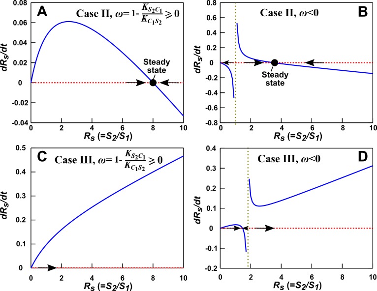
If $\omega =1-K_{S_2{C}_1}/K_{C_1{S}_2}\ge 0$ (Figure 3—figure supplement 3A): When ${\displaystyle R_S<R_S^{\ast }}$, $d{R}_S/dt$ is positive. When ${\displaystyle R_S>R_S^{\ast }}$, $d{R}_S/dt$ is negative. Thus, wherever the initial ${\displaystyle R_S}$, it will always converge toward the only steady state ${\displaystyle R_S^{\ast }}$ of the mechanistic model.

If $\omega <0$ (Figure 3—figure supplement 3B): $\omega +\psi R_S=0$ or $R_S=-\omega /\psi$ creates singularity. Pairwise model ${\displaystyle R_S}$ will only converge toward the mechanistic model steady state if

$$R_S\left(0\right)>-\omega /\psi$$ (44)

• Case III ($r_{10}<r_{20}$): ${\displaystyle R_S}$ increases exponentially in mechanistic model (Equation 9). Thus, ${\displaystyle C_1}$ will decline toward zero as C₁ is consumed by S₂ whose relative abundance over S₁ exponentially increases. Hence, according to Equation 9, ${\displaystyle R_S}$ eventually increases exponentially at a rate of $r_{20}-r_{10}$.

If $\omega \ge 0$ (Figure 3—figure supplement 3C): Equation 43 $\frac{d{R}_S}{dt}=\left(r_{20}+\frac{r_{S_2{C}_1}}{\omega +\psi R_S}-r_{10}\right)R_S$>0. Thus, Equation 43, which is based on alternative pairwise model, also predicts that ${\displaystyle R_S}$ will eventually increase exponentially at a rate of $r_{20}-r_{10}$, similar to the mechanistic model.

If $\omega <0$ (Figure 3—figure supplement 3D): $R_S\left(0\right)>-\omega /\psi$ (Equation 44) is required for unbounded increase in ${\displaystyle R_S}$ (similar to the mechanistic model). Otherwise, ${\displaystyle R_S}$ converges to an erroneous value instead.

Conditions under which a saturable L-V pairwise model can represent one species influencing another via two reusable mediators

Here, we examine a simple case where S₁ releases reusable C₁ and C₂, and C₁ and C₂ additively affect the growth of S₂ (see example in Figure 5). Similar to Figure 3A, the mechanistic model is:

$${\displaystyle \{\begin{array}{ll}{S}_1& =S_{10}\exp \left(r_{10}t\right)\\ \frac{d{S}_2}{dt}& =\left(r_{20}+\frac{r_{S_2{C}_1}{S}_1}{S_1+K_{S_2{C}_1}{r}_{10}/{\beta }_{C_1{S}_1}}+\frac{r_{S_2{C}_2}{S}_1}{S_1+K_{S_2{C}_2}{r}_{10}/{\beta }_{C_2{S}_1}}\right)S_2\end{array}}$$ (45)

Now the question is whether the saturable L-V pairwise model

$${\displaystyle \{\begin{array}{ll}{S}_1& =S_{10}\exp \left(r_{10}t\right)\\ \frac{d{S}_2}{dt}& =\left(r_{20}+r_{21}\frac{S_1}{S_1+K_{21}}\right)S_2\end{array}}$$

can be a good approximation.

For simplicity, let’s define $K_{C1}=K_{S_2{C}_1}{r}_{10}/{\beta }_{C_1{S}_1}$ and $K_{C2}=K_{S_2{C}_2}{r}_{10}/{\beta }_{C_2{S}_1}$. Small ${\displaystyle K_{Ci}}$ means large potency (e.g. small ${\displaystyle K_{C2}}$ can be caused by small $K_{S_2{C}_2}$ which means low ${\displaystyle C_2}$ required to achieve half maximal effect on S₂, and/or large synthesis rate ${\beta }_{C_2{S}_1}$). Since ${\displaystyle S_1}$ from pairwise and mechanistic models are identical, we have

$${\displaystyle \begin{array}{ll}& \overline{D}=\frac{1}{2T}{\int }_T|{\log }_{10}\left(S_{2,pair}\right)-{\log }_{10}\left(S_{2,mech}\right)|dt\\ & =\frac{1}{2T\ln \left(10\right)}{\int }_T|\ln \left(S_{2,pair}\right)-\ln \left(S_{2,mech}\right)|dt\\ & =\frac{1}{2T\ln \left(10\right)}{\int }_T|{\int }_t\left|\left(r_{20}+r_{21}\frac{S_1}{S_1+K_{21}}\right)d\tau -{\int }_t\left(r_{20}+\frac{r_{S_2{C}_1}{S}_1}{S_1+K_{C1}}+\frac{r_{S_2{C}_2}{S}_1}{S_1+K_{C2}}\right)d\tau \right|dt\\ & =\frac{1}{2T\ln \left(10\right)}{\int }_T\left|{\int }_t\left[r_{21}\frac{S_1}{S_1+K_{21}}-\left(\frac{r_{S_2{C}_1}{S}_1}{S_1+K_{C1}}+\frac{r_{S_2{C}_2}{S}_1}{S_1+K_{C2}}\right)\right]d\tau \right|dt\end{array}}$$ (46)

$\overline{D}$ can be close to zero when (i) $K_{C1}\approx K_{C2}$ or (ii) $\frac{r_{S_2{C}_1}{S}_1}{S_1+K_{C1}}$ and $\frac{r_{S_2{C}_2}{S}_1}{S_1+K_{C2}}$(effects of C₁ and C₂ on S₂) differ dramatically in magnitude. For (ii), without loss of generality, suppose that the effect of C₂ on S₂ can be neglected. This can be achieved if (iia) $r_{S_2{C}_2}$ is much smaller than $r_{S_2{C}_1}$, or (iib) $K_{C_2}$ is large compared to S₁.

Competitive commensal interaction

For the community in Figure 6A, our mechanistic model is:

$${\displaystyle \begin{array}{ll}\frac{d{S}_1}{dt}& =\left(r_{10}+r_{S_1{C}_1}\frac{C_1}{C_1+K_{S_1{C}_1}}\right)S_1\\ \frac{d{S}_2}{dt}& =\left[r_{20}+r_{S_2{C}_{1,2}}\frac{\left(C_1/K_{S_2{C}_1}\right)\left(C_2/K_{S_2{C}_2}\right)}{C_1/K_{S_2{C}_1}+C_2/K_{S_2{C}_2}}\left(\frac{1}{C_1/K_{S_2{C}_1}+1}+\frac{1}{C_2/K_{S_2{C}_2}+1}\right)\right]S_2\\ \frac{d{C}_1}{dt}& ={\beta }_0-{\alpha }_{C_1{S}_1}{r}_{S_1{C}_1}\frac{C_1}{C_1+K_{S_1{C}_1}}{S}_1-{\alpha }_{C_1{S}_2}{r}_{S_2{C}_{1,2}}\frac{\frac{C_1}{K_{S_2{C}_1}}\frac{C_2}{K_{S_2{C}_2}}}{\frac{C_1}{K_{S_2{C}_1}}+\frac{C_2}{K_{S_2{C}_2}}}\left(\frac{1}{\frac{C_1}{K_{S_2{C}_1}}+1}+\frac{1}{\frac{C_2}{K_{S_2{C}_2}}+1}\right)S_2\\ \frac{d{C}_2}{dt}& ={\beta }_{C_2{S}_1}{S}_1-{\alpha }_{C_2{S}_2}{r}_{S_2{C}_{1,2}}\frac{\left(C_1/K_{S_2{C}_1}\right)\left(C_2/K_{S_2{C}_2}\right)}{C_1/K_{S_2{C}_1}+C_2/K_{S_2{C}_2}}\left(\frac{1}{C_1/K_{S_2{C}_1}+1}+\frac{1}{C_2/K_{S_2{C}_2}+1}\right)S_2\end{array}}$$ (47)

Here, ${\displaystyle S_1}$ and ${\displaystyle S_2}$ are the densities of the two species; ${\displaystyle r_{i0}}$ is the basal net growth rate of S_i (negative, representing death in the absence of the essential shared resource C₁); C₁ is supplied at a constant rate ${\displaystyle {\beta }_0}$; ${\beta }_{C_2}{}_{S_1}$is the production rate of C₂ by S₁; ${\alpha }_{C_i}{}_{S_j}$ is the amount of resource C_i consumed to produce a new S_j cell.

The growth of S₂ is controlled by ${\displaystyle C_1}$ and ${\displaystyle C_2}$. When ${\displaystyle C_1}$ is limiting (${\displaystyle C_1/K_{S_2{C}_1}\ll C_2/K_{S_2{C}_2}}$), the fitness influence of the two chemicals on S₂ becomes:

$${\displaystyle \begin{array}{ll}& r_{S_2{C}_{1,2}}\frac{\left(C_1/K_{S_2{C}_1}\right)\left(C_2/K_{S_2{C}_2}\right)}{C_1/K_{S_2{C}_1}+C_2/K_{S_2{C}_2}}\left(\frac{1}{C_1/K_{S_2{C}_1}+1}+\frac{1}{C_2/K_{S_2{C}_2}+1}\right)\\ & \approx r_{S_2{C}_{1,2}}\frac{\left(C_1/K_{S_2{C}_1}\right)\left(C_2/K_{S_2{C}_2}\right)}{C_2/K_{S_2{C}_2}}\left(\frac{1}{C_1/K_{S_2{C}_1}+1}\right)=r_{S_2{C}_{1,2}}\frac{C_1/K_{S_2{C}_1}}{C_1/K_{S_2{C}_1}+1}=r_{S_2{C}_{1,2}}\frac{C_1}{C_1+K_{S_2{C}_1}}\end{array}}$$

which is the standard Monod equation. A similar argument holds for limiting ${\displaystyle C_2}$. We have intentionally chosen very large $K_{S_2}{}_{C_2}$ to ensure that the fitness effect of C₂ on S₂ is linear with respect to ${\displaystyle C_2}$. This way, we minimize the number of pairwise model parameters that need to be estimated.

For our L-V pairwise model, to capture intra-species competition, we use

$$\frac{d{S}_i}{dt}=b_{i0}\left(1-\frac{S_i}{{\kappa }_i}\right)S_i-d_i{S}_i$$

where non-negative ${\displaystyle b_{i0}}$ represents the maximal birth rate of S_i at nearly zero population density (no competition), and non-negative ${\displaystyle d_i}$ represents the constant death rate of S_i. Positive ${\kappa }_i$ is the ‘carrying capacity’ imposed by the limiting resource, and is the ${\displaystyle S_i}$ at which birth rate becomes zero. This equation can be simplified to:

$${\displaystyle \frac{d{S}_i}{dt}=\left(b_{i0}-d_i\right)\left[1-\frac{S_i}{{\kappa }_i\left(1-d_i/b_{i0}\right)}\right]S_i=r_{i0}\left[1-\frac{S_i}{{\mathrm{\Lambda }}_i}\right]S_i.}$$

When ${\Lambda }_i$>0 (i.e. when $b_{i0}>d_i$), this resembles standard L-V model traditionally used for competitive interactions (compare to Equation 2; Gause, 1934; Thébault and Fontaine, 2010; Mougi and Kondoh, 2012).

Thus, for the competitive commensal community, we have:

$${\displaystyle \begin{array}{l}\frac{d{S}_1}{dt}=b_{10}\left(1-\frac{S_1}{{\mathrm{\Lambda }}_{11}}-\frac{S_2}{{\mathrm{\Lambda }}_{12}}\right)S_1-d_1{S}_1\\ \frac{d{S}_2}{dt}=\left(b_{20}+r_{21}{S}_1\right)\left(1-\frac{S_1}{{\mathrm{\Lambda }}_{21}}-\frac{S_2}{{\mathrm{\Lambda }}_{22}}\right)S_2-d_2{S}_2\end{array}}$$ (48)

Here, birth rate of each species is reduced by competition from the two species, and ${\Lambda }_{ij}$ is the carrying capacity such that a single S_i individual will have a zero birth rate when encountering a total of ${\Lambda }_{ij}$ individuals of S_j. For S₂, We used $\left(b_{20}+r_{21}{S}_1\right)\left(1-\frac{S_1}{{\Lambda }_{21}}-\frac{S_2}{{\Lambda }_{22}}\right)S_2$ instead of $b_{20}\left(1-\frac{S_1}{{\Lambda }_{21}}-\frac{S_2}{{\Lambda }_{22}}\right)S_2+r_{21}{S}_1{S}_2$ so that when the shared resource is exhausted (i.e. $1-\frac{S_1}{{\Lambda }_{21}}-\frac{S_2}{{\Lambda }_{22}}$=0), S₂ does not keep growing due to the presence of S₁.

Funding Statement

The funders had no role in study design, data collection and interpretation, or the decision to submit the work for publication.

Funding Information

This paper was supported by the following grants:

• Boston College to Babak Momeni.

• NIH Office of the Director to Babak Momeni, Wenying Shou.

• W. M. Keck Foundation to Babak Momeni, Li Xie, Wenying Shou.

• Fred Hutchinson Cancer Research Center to Li Xie, Wenying Shou.

Additional files

Source code 1. Calculates the cost function for monocultures (i.e. the difference between the target mechanistic model dynamics and the dynamics obtained from the pairwise model).

DOI: http://dx.doi.org/10.7554/eLife.25051.034

Source code 2. Calculates the cost function for communities (i.e. the difference between the target mechanistic model dynamics and the dynamics obtained from the saturable L-V pairwise model).

DOI: http://dx.doi.org/10.7554/eLife.25051.035

Source code 3. Calculates the cost function for communities (i.e. the difference between the target mechanistic model dynamics and the dynamics obtained from the alternative pairwise model).

DOI: http://dx.doi.org/10.7554/eLife.25051.036

Source code 4. Returns growth dynamics for monocultures, based on the mechanistic model.

DOI: http://dx.doi.org/10.7554/eLife.25051.037

Source code 5. Returns growth dynamics for communities of multiple species, based on the mechanistic model.

DOI: http://dx.doi.org/10.7554/eLife.25051.038

Source code 6. Returns growth dynamics for communities of multiple species, based on the saturable L-V pairwise model.

DOI: http://dx.doi.org/10.7554/eLife.25051.039

Source code 7. Returns growth dynamics for communities of multiple species, based on the alternative pairwise model.

DOI: http://dx.doi.org/10.7554/eLife.25051.040

Source code 8. Estimates monoculture parameters of pairwise model (Step 1).

DOI: http://dx.doi.org/10.7554/eLife.25051.041

Source code 9. Estimates saturable L-V pairwise model interaction parameters (Step 2).

DOI: http://dx.doi.org/10.7554/eLife.25051.042

Source code 10. Estimates alternative pairwise model interaction parameters (Step 2).

DOI: http://dx.doi.org/10.7554/eLife.25051.043

Source code 11. Estimates saturable L-V pairwise model interaction parameters (r₂₁ and K₂₁) in cases where we know that S₂ is only affected by S₁, to accelerate optimization.

DOI: http://dx.doi.org/10.7554/eLife.25051.044

Source code 12. Estimates alternative pairwise model interaction parameter (r₂₁) in cases where we know that S₂ is only affected by S₁ and that K_S2C1=K_C1S2 to accelerate optimization.

DOI: http://dx.doi.org/10.7554/eLife.25051.045

Source code 13. Returns growth dynamics for communities of two species competing for an environmental resource while engaging in an additional interaction, based on the logistic L-V pairwise model (Figure 6).

DOI: http://dx.doi.org/10.7554/eLife.25051.046

Source code 14. Estimates logistic L-V pairwise model interaction parameters for communities of two species competing for an environmental resource while engaging in an additional interaction, and compares community dynamics from pairwise and mechanistic models (Figure 6).

DOI: http://dx.doi.org/10.7554/eLife.25051.047

Source code 15. Defines differential equations when using Matlab’s ODE23 solver to calculate community dynamics.

DOI: http://dx.doi.org/10.7554/eLife.25051.048

Source code 16. Example of using Matlab ODE23 solver for calculating community dynamics.

DOI: http://dx.doi.org/10.7554/eLife.25051.049

References

- Allesina S, Tang S. Stability criteria for complex ecosystems. Nature. 2012;483:205–208. doi: 10.1038/nature10832. [DOI] [PubMed] [Google Scholar]
- Bader FG. Analysis of double-substrate limited growth. Biotechnology and Bioengineering. 1978;20:183–202. doi: 10.1002/bit.260200203. [DOI] [PubMed] [Google Scholar]
- Bairey E, Kelsic ED, Kishony R. High-order species interactions shape ecosystem diversity. Nature Communications. 2016;7:12285. doi: 10.1038/ncomms12285. [DOI] [PMC free article] [PubMed] [Google Scholar]
- Bayer EA, Lamed R. Ultrastructure of the cell surface cellulosome of Clostridium thermocellum and its interaction with cellulose. Journal of Bacteriology. 1986;167:828–836. doi: 10.1128/jb.167.3.828-836.1986. [DOI] [PMC free article] [PubMed] [Google Scholar]
- Billick I, Case TJ. Higher order interactions in Ecological Communities: what are they and how can they be detected? Ecology. 1994;75:1529–1543. doi: 10.2307/1939614. [DOI] [Google Scholar]
- BiologyEOC PopulationChanges. 2016. [June 1 2016]. https://biologyeoc.wikispaces.com/PopulationChanges
- Bradshaw DJ, Homer KA, Marsh PD, Beighton D. Metabolic cooperation in oral microbial communities during growth on mucin. Microbiology. 1994;140:3407–3412. doi: 10.1099/13500872-140-12-3407. [DOI] [PubMed] [Google Scholar]
- Case TJ, Bender EA. Testing for higher order interactions. The American Naturalist. 1981;118:920–929. doi: 10.1086/283885. [DOI] [Google Scholar]
- Case TJ, Casten RG. Global stability and multiple domains of attraction in ecological systems. The American Naturalist. 1979;113:705–714. doi: 10.1086/283427. [DOI] [Google Scholar]
- Chen H, Fujita M, Feng Q, Clardy J, Fink GR. Tyrosol is a quorum-sensing molecule in candida albicans. PNAS. 2004;101:5048–5052. doi: 10.1073/pnas.0401416101. [DOI] [PMC free article] [PubMed] [Google Scholar]
- Chesson P. MacArthur's consumer-resource model. Theoretical Population Biology. 1990;37:26–38. doi: 10.1016/0040-5809(90)90025-Q. [DOI] [Google Scholar]
- Coyte KZ, Schluter J, Foster KR. The ecology of the microbiome: networks, competition, and stability. Science. 2015;350:663–666. doi: 10.1126/science.aad2602. [DOI] [PubMed] [Google Scholar]
- Czárán TL, Hoekstra RF, Pagie L. Chemical warfare between microbes promotes biodiversity. PNAS. 2002;99:786–790. doi: 10.1073/pnas.012399899. [DOI] [PMC free article] [PubMed] [Google Scholar]
- D'Onofrio A, Crawford JM, Stewart EJ, Witt K, Gavrish E, Epstein S, Clardy J, Lewis K. Siderophores from neighboring organisms promote the growth of uncultured bacteria. Chemistry & Biology. 2010;17:254–264. doi: 10.1016/j.chembiol.2010.02.010. [DOI] [PMC free article] [PubMed] [Google Scholar]
- Dormann CF, Roxburgh SH. Experimental evidence rejects pairwise modelling approach to coexistence in plant communities. Proceedings of the Royal Society B: Biological Sciences. 2005;272:1279–1285. doi: 10.1098/rspb.2005.3066. [DOI] [PMC free article] [PubMed] [Google Scholar]
- Duan K, Sibley CD, Davidson CJ, Surette MG. Chemical interactions between organisms in microbial communities. Contributions to Microbiology. 2009;16:1–17. doi: 10.1159/000219369. [DOI] [PubMed] [Google Scholar]
- Durrett R, Levin S. The importance of being discrete (and spatial) Theoretical Population Biology. 1994;46:363–394. doi: 10.1006/tpbi.1994.1032. [DOI] [Google Scholar]
- Faust K, Raes J. Microbial interactions: from networks to models. Nature Reviews Microbiology. 2012;10:538–550. doi: 10.1038/nrmicro2832. [DOI] [PubMed] [Google Scholar]
- Felix CR, Ljungdahl LG. The cellulosome: the exocellular organelle of Clostridium. Annual Review of Microbiology. 1993;47:791–819. doi: 10.1146/annurev.mi.47.100193.004043. [DOI] [PubMed] [Google Scholar]
- Freilich S, Zarecki R, Eilam O, Segal ES, Henry CS, Kupiec M, Gophna U, Sharan R, Ruppin E. Competitive and cooperative metabolic interactions in bacterial communities. Nature Communications. 2011;2:589. doi: 10.1038/ncomms1597. [DOI] [PubMed] [Google Scholar]
- Friedman J, Higgins LM, Gore J. Community structure follows simple assembly rules in microbial microcosms. Nature Ecology & Evolution. 2017;1:0109. doi: 10.1038/s41559-017-0109. [DOI] [PubMed] [Google Scholar]
- Gause GF. The Struggle for Existence. Baltimore: Williams & Wilkins; 1934. [Google Scholar]
- Ghuysen JM. Serine beta-lactamases and penicillin-binding proteins. Annual Review of Microbiology. 1991;45:37–67. doi: 10.1146/annurev.mi.45.100191.000345. [DOI] [PubMed] [Google Scholar]
- Gopalsamy K. Stability and Oscillations in Delay Differential Equations of Population Dynamics. Springer Science & Business Media; 1992. [Google Scholar]
- Green R, Shou W. Modeling community population dynamics with the open-source language R. Methods in Molecular Biology. 2014;1151:209–231. doi: 10.1007/978-1-4939-0554-6_15. [DOI] [PubMed] [Google Scholar]
- Guo X, Boedicker JQ. The contribution of High-Order metabolic interactions to the global activity of a four-species microbial community. PLoS Computational Biology. 2016;12:e1005079. doi: 10.1371/journal.pcbi.1005079. [DOI] [PMC free article] [PubMed] [Google Scholar]
- Hamilton IR, Ng SKC. Stimulation of glycolysis through lactate consumption in a resting cell mixture of Streptococcus salivarius and Veillonella parvula. FEMS Microbiology Letters. 1983;20:61–65. doi: 10.1111/j.1574-6968.1983.tb00090.x. [DOI] [Google Scholar]
- Hermsen R, Okano H, You C, Werner N, Hwa T. A growth-rate composition formula for the growth of E.coli on co-utilized carbon substrates. Molecular Systems Biology. 2015;11:801. doi: 10.15252/msb.20145537. [DOI] [PMC free article] [PubMed] [Google Scholar]
- Jakubovics NS, Gill SR, Vickerman MM, Kolenbrander PE. Role of hydrogen peroxide in competition and cooperation between Streptococcus gordonii and Actinomyces naeslundii. FEMS Microbiology Ecology. 2008;66:637–644. doi: 10.1111/j.1574-6941.2008.00585.x. [DOI] [PMC free article] [PubMed] [Google Scholar]
- Jakubovics NS. Talk of the town: interspecies communication in oral biofilms. Molecular Oral Microbiology. 2010;25:4–14. doi: 10.1111/j.2041-1014.2009.00563.x. [DOI] [PubMed] [Google Scholar]
- Johnson EA, Sakajoh M, Halliwell G, Madia A, Demain AL. Saccharification of complex cellulosic substrates by the cellulase system from Clostridium thermocellum. Applied and Environmental Microbiology. 1982;43:1125–1132. doi: 10.1128/aem.43.5.1125-1132.1982. [DOI] [PMC free article] [PubMed] [Google Scholar]
- Kato S, Haruta S, Cui ZJ, Ishii M, Igarashi Y. Stable coexistence of five bacterial strains as a cellulose-degrading community. Applied and Environmental Microbiology. 2005;71:7099–7106. doi: 10.1128/AEM.71.11.7099-7106.2005. [DOI] [PMC free article] [PubMed] [Google Scholar]
- Kato S, Haruta S, Cui ZJ, Ishii M, Igarashi Y. Network relationships of bacteria in a stable mixed culture. Microbial Ecology. 2008;56:403–411. doi: 10.1007/s00248-007-9357-4. [DOI] [PubMed] [Google Scholar]
- Kau AL, Ahern PP, Griffin NW, Goodman AL, Gordon JI. Human nutrition, the gut microbiome and the immune system. Nature. 2011;474:327–336. doi: 10.1038/nature10213. [DOI] [PMC free article] [PubMed] [Google Scholar]
- Kelsic ED, Zhao J, Vetsigian K, Kishony R. Counteraction of antibiotic production and degradation stabilizes microbial communities. Nature. 2015;521:516–519. doi: 10.1038/nature14485. [DOI] [PMC free article] [PubMed] [Google Scholar]
- Kim KS, Lee S, Ryu CM. Interspecific bacterial sensing through airborne signals modulates locomotion and drug resistance. Nature Communications. 2013;4:1809. doi: 10.1038/ncomms2789. [DOI] [PubMed] [Google Scholar]
- Kolenbrander PE. Oral microbial communities: biofilms, interactions, and genetic systems. Annual Review of Microbiology. 2000;54:413–437. doi: 10.1146/annurev.micro.54.1.413. [DOI] [PubMed] [Google Scholar]
- Kuramitsu HK, He X, Lux R, Anderson MH, Shi W. Interspecies interactions within oral microbial communities. Microbiology and Molecular Biology Reviews. 2007;71:653–670. doi: 10.1128/MMBR.00024-07. [DOI] [PMC free article] [PubMed] [Google Scholar]
- Lendenmann U, Egli T. Kinetic models for the growth of Escherichia coli with mixtures of sugars under carbon-limited conditions. Biotechnology and Bioengineering. 1998;59:99–107. doi: 10.1002/(SICI)1097-0290(19980705)59:1<99::AID-BIT13>3.0.CO;2-Y. [DOI] [PubMed] [Google Scholar]
- Levine SH. Competitive interactions in ecosystems. The American Naturalist. 1976;110:903–910. doi: 10.1086/283116. [DOI] [Google Scholar]
- Levins R. The Strategy of Model Building in Population Biology. American Scientist. 1966;54:421–431. [Google Scholar]
- Li XY, Pietschke C, Fraune S, Altrock PM, Bosch TC, Traulsen A. Which games are growing bacterial populations playing? Journal of the Royal Society, Interface. 2015;12:20150121. doi: 10.1098/rsif.2015.0121. [DOI] [PMC free article] [PubMed] [Google Scholar]
- MacArthur R. Species packing and competitive equilibrium for many species. Theoretical Population Biology. 1970;1:1–11. doi: 10.1016/0040-5809(70)90039-0. [DOI] [PubMed] [Google Scholar]
- Mankad T, Bungay HR. Model for microbial growth with more than one limiting nutrient. Journal of Biotechnology. 1988;7:161–166. doi: 10.1016/0168-1656(88)90062-4. [DOI] [Google Scholar]
- Marino S, Baxter NT, Huffnagle GB, Petrosino JF, Schloss PD. Mathematical modeling of primary succession of murine intestinal Microbiota. PNAS. 2014;111:439–444. doi: 10.1073/pnas.1311322111. [DOI] [PMC free article] [PubMed] [Google Scholar]
- Marsh PD, Bradshaw DJ. Physiological approaches to the control of oral biofilms. Advances in Dental Research. 1997;11:176–185. doi: 10.1177/08959374970110010901. [DOI] [PubMed] [Google Scholar]
- May RM. Will a large complex system be stable? Nature. 1972;238:413–414. doi: 10.1038/238413a0. [DOI] [PubMed] [Google Scholar]
- Momeni B, Brileya KA, Fields MW, Shou W. Strong inter-population cooperation leads to partner intermixing in microbial communities. eLife. 2013;2:e00230. doi: 10.7554/eLife.00230. [DOI] [PMC free article] [PubMed] [Google Scholar]
- Mougi A, Kondoh M. Diversity of interaction types and ecological community stability. Science. 2012;337:349–351. doi: 10.1126/science.1220529. [DOI] [PubMed] [Google Scholar]
- Mounier J, Monnet C, Vallaeys T, Arditi R, Sarthou AS, Hélias A, Irlinger F. Microbial interactions within a cheese microbial community. Applied and Environmental Microbiology. 2008;74:172–181. doi: 10.1128/AEM.01338-07. [DOI] [PMC free article] [PubMed] [Google Scholar]
- Pascual MA, Kareiva P. Predicting the outcome of competition using experimental data: maximum likelihood and bayesian approaches. Ecology. 1996;77:337–349. doi: 10.2307/2265613. [DOI] [Google Scholar]
- Pimm SL. Food Webs. Netherlands: Springer; 1982. pp. 1–11. [Google Scholar]
- Round JL, Mazmanian SK. The gut microbiota shapes intestinal immune responses during health and disease. Nature Reviews Immunology. 2009;9:313–323. doi: 10.1038/nri2515. [DOI] [PMC free article] [PubMed] [Google Scholar]
- Schmitz OJ, Krivan V, Ovadia O. Trophic cascades: the primacy of trait-mediated indirect interactions. Ecology Letters. 2004;7:153–163. doi: 10.1111/j.1461-0248.2003.00560.x. [DOI] [Google Scholar]
- Schwarz WH. The cellulosome and cellulose degradation by anaerobic bacteria. Applied Microbiology and Biotechnology. 2001;56:634–649. doi: 10.1007/s002530100710. [DOI] [PubMed] [Google Scholar]
- Seghezzo L, Zeeman G, van Lier JB, Hamelers HVM, Lettinga G. A review: the anaerobic treatment of sewage in UASB and EGSB reactors. Bioresource Technology. 1998;65:175–190. doi: 10.1016/S0960-8524(98)00046-7. [DOI] [Google Scholar]
- Stams AJ. Metabolic interactions between anaerobic bacteria in methanogenic environments. Antonie Van Leeuwenhoek. 1994;66:271–294. doi: 10.1007/BF00871644. [DOI] [PubMed] [Google Scholar]
- Stanton ML. Interacting guilds: moving beyond the pairwise perspective on mutualisms. The American Naturalist. 2003;162:S10–S23. doi: 10.1086/378646. [DOI] [PubMed] [Google Scholar]
- Stein RR, Bucci V, Toussaint NC, Buffie CG, Rätsch G, Pamer EG, Sander C, Xavier JB. Ecological modeling from time-series inference: insight into dynamics and stability of intestinal microbiota. PLoS Computational Biology. 2013;9:e1003388. doi: 10.1371/journal.pcbi.1003388. [DOI] [PMC free article] [PubMed] [Google Scholar]
- Suweis S, Simini F, Banavar JR, Maritan A. Emergence of structural and dynamical properties of ecological mutualistic networks. Nature. 2013;500:449–452. doi: 10.1038/nature12438. [DOI] [PubMed] [Google Scholar]
- Thébault E, Fontaine C. Stability of ecological communities and the architecture of mutualistic and trophic networks. Science. 2010;329:853–856. doi: 10.1126/science.1188321. [DOI] [PubMed] [Google Scholar]
- Tilman D. The importance of the mechanisms of interspecific competition. The American Naturalist. 1987;129:769–774. doi: 10.1086/284672. [DOI] [Google Scholar]
- Traxler MF, Watrous JD, Alexandrov T, Dorrestein PC, Kolter R. Interspecies interactions stimulate diversification of the Streptomyces coelicolor secreted metabolome. mBio. 2013;4:e00459-13. doi: 10.1128/mBio.00459-13. [DOI] [PMC free article] [PubMed] [Google Scholar]
- van Hijum SA, Vaughan EE, Vogel RF. Application of state-of-art sequencing technologies to indigenous food fermentations. Current Opinion in Biotechnology. 2013;24:178–186. doi: 10.1016/j.copbio.2012.08.004. [DOI] [PubMed] [Google Scholar]
- Vandermeer JH. The competitive structure of communities: an experimental approach with protozoa. Ecology. 1969;50:362–371. doi: 10.2307/1933884. [DOI] [Google Scholar]
- Vetsigian K, Jajoo R, Kishony R. Structure and evolution of Streptomyces interaction networks in soil and in silico. PLoS Biology. 2011;9:e1001184. doi: 10.1371/journal.pbio.1001184. [DOI] [PMC free article] [PubMed] [Google Scholar]
- Volterra V. Variations and fluctuations of the number of individuals in animal species living together. Journal Du Conseil Conseil Permanent International Pour Exploration De La Mer. 1926;1931:3–51. [Google Scholar]
- Wangersky PJ. Lotka-Volterra population models. Annual Review of Ecology and Systematics. 1978;9:189–218. doi: 10.1146/annurev.es.09.110178.001201. [DOI] [Google Scholar]
- Werner EE, Peacor SD. A review of trait-mediated indirect interactions in ecological communities. Ecology. 2003;84:1083–1100. doi: 10.1890/0012-9658(2003)084[1083:AROTII]2.0.CO;2. [DOI] [Google Scholar]
- Widder S, Allen RJ, Pfeiffer T, Curtis TP, Wiuf C, Sloan WT, Cordero OX, Brown SP, Momeni B, Shou W, Kettle H, Flint HJ, Haas AF, Laroche B, Kreft JU, Rainey PB, Freilich S, Schuster S, Milferstedt K, van der Meer JR, Groβkopf T, Huisman J, Free A, Picioreanu C, Quince C, Klapper I, Labarthe S, Smets BF, Wang H, Soyer OS, Isaac Newton Institute Fellows Challenges in microbial ecology: building predictive understanding of community function and dynamics. The ISME Journal. 2016;10:2557–2568. doi: 10.1038/ismej.2016.45. [DOI] [PMC free article] [PubMed] [Google Scholar]
- Wootton JT. Indirect effects and habitat use in an intertidal community: interaction chains and interaction modifications. The American Naturalist. 1993;141:71–89. doi: 10.1086/285461. [DOI] [Google Scholar]
- Wootton JT. The nature and consequences of indirect effects in ecological communities. Annual Review of Ecology and Systematics. 1994;25:443–466. doi: 10.1146/annurev.es.25.110194.002303. [DOI] [Google Scholar]
- Wootton JT. Indirect effects in complex ecosystems: recent progress and future challenges. Journal of Sea Research. 2002;48:157–172. doi: 10.1016/S1385-1101(02)00149-1. [DOI] [Google Scholar]
- Worthen WB, Moore JL. Higher-Order interactions and indirect effects: a resolution using laboratory Drosophila communities. The American Naturalist. 1991;138:1092–1104. doi: 10.1086/285271. [DOI] [Google Scholar]
- Yang YL, Xu Y, Straight P, Dorrestein PC. Translating metabolic exchange with imaging mass spectrometry. Nature Chemical Biology. 2009;5:885–887. doi: 10.1038/nchembio.252. [DOI] [PMC free article] [PubMed] [Google Scholar]