Defining a Cancer Dependency Map

SUMMARY

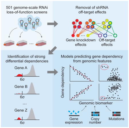
Most human epithelial tumors harbor numerous alterations, making it difficult to predict which genes are required for tumor survival. To systematically identify cancer dependencies, we analyzed 501 genome-scale loss-of-function screens performed in diverse human cancer cell lines. We developed DEMETER, an analytical framework that segregates on-from off-target effects of RNAi. 769 genes were differentially required in subsets of these cell lines at a threshold of six standard deviations from the mean. We found predictive models for 426 dependencies (55%) by nonlinear regression modeling considering 66,646 molecular features. Many dependencies fall into a limited number of classes, and unexpectedly, in 82% of models, the top biomarkers were expression-based. We demonstrated the basis behind one such predictive model linking hypermethylation of the UBB ubiquitin gene to a dependency on UBC. Together, these observations provide a foundation for a cancer dependency map that facilitates the prioritization of therapeutic targets.

Graphical Abstract

INTRODUCTION

Multiple genetic or epigenetic changes are required to program the malignant state. Although we now have an initial view of the landscape of genetic alterations that occur in cancers, our understanding of the biological impact of these features and how they conspire to induce specific tumor vulnerabilities is largely incomplete. As a result, the use of genetic information from tumors to enable cancer precision medicine is limited.

One approach to identifying genes essential for cancer cell proliferation/survival is to perform systematic loss of function screens in a large number of well-annotated cell lines representing the heterogeneity of tumors. We and others have demonstrated that these experiments are feasible (Aguirre et al., 2016; Cheung et al., 2011; Cowley et al., 2014; Luo et al., 2008; Marcotte et al., 2012; Marcotte et al., 2016), and the interrogation of single or multiple lineages has identified new oncogenes and genes essential for cell proliferation or the activity of specific signaling pathways (Aguirre et al., 2016; Barbie et al., 2009; Cheung et al., 2011; Cowley et al., 2014; Luo et al., 2008; Marcotte et al., 2012; Marcotte et al., 2016). However, these RNA interference (RNAi) and CRISPR-Cas9 experiments have been limited by off-target effects of such reagents (Aguirre et al., 2016; Birmingham et al., 2006; Buehler et al., 2012b; Jackson and Linsley, 2004; Munoz et al., 2016) and also by an insufficient number of cell line models to adequately represent the full spectrum of the molecular complexity of cancer.

Here we have integrated a large number of genome-scale RNAi-based loss-of-function screens to facilitate the interrogation of gene function. Using this dataset, we developed an analytical approach that quantifies on- and off-target effects of each RNAi reagent. By combining this information with a comprehensive genomic characterization of these cell lines, we systematically predicted cancer dependencies, thereby establishing an initial framework for a cancer dependencies map.

RESULTS

Overcoming off-target effects of RNAi to accurately infer cancer dependencies

Although RNAi is a powerful technique, microRNA (miRNA) “seed”-based off-target effects have been reported to confound experimental interpretation (Birmingham et al., 2006; Buehler et al., 2012b; Jackson et al., 2006). We hypothesized that explicitly modeling onand off-target effects induced by RNAi in a large set of cancer cell lines would provide the means to estimate the on-target effects of suppressing genes in these experiments. We first built on our previous study of 216 human cancer cell lines (Cowley et al., 2014) by screening an additional 285 cell lines. In brief these screens consist of transducing each cell line with a genome-scale library of ~100,000 shRNAs at low MOI in ~60M cells for each of 4 replicates, so that each cell gets one shRNA, passaging the cells for 16 doublings, up to 40 days, and then assessing by massively parallel sequencing the depletion of each shRNA from the cell population versus its relative abundance in the original pooled library of shRNA plasmids. The genes targeted by the most depleted shRNAs are inferred to be most essential for proliferation/viability (see Methods for details). The resulting compiled dataset of genome-scale screens in 501 cell lines includes a wide diversity of cancer types (Figure 1A; Table S1).

Figure 1. Computational segregation of on- and off-target effects of RNAi.

(A) Tumor types by their contribution to cancer mortality (left) and their cancer cell line representation in the reported dataset (right). (B) Distributions of Pearson correlation coefficients for pairs of shRNA viability profiles before (left) and after (right) removal of inferred seed effects and selection of effective shRNAs (n > 12,000) by DEMETER. Pairs of shRNAs selected randomly (blue lines), targeting the same gene (orange) and sharing a seed sequence (green). (C) Schematic representation of DEMETER and its computational model. Gene- and seed-related effects are estimated from shRNA depletion data. The color of inner circles represents the shRNA target gene and the color of outer circles represents the shRNAs seed sequence. (D) For the top 0.1% most depleted shRNA readouts and the top 0.1% DEMETER gene dependency scores across the whole dataset, the fraction of data points corresponding to a cell line not expressing the target gene. (E) A heatmap depicts the dependency scores (rows) across 501 screened lines (columns) for PIK3CA and the 7 genes that have significantly correlated dependency profiles (z-score > 3). These data were used to plot a gene network, with each edge representing a significant correlation between a pair of dependency profiles. Genes are colored by functional classes. The same analysis was used to generate gene networks for PTK2 (F) and MED12 (G).

First, we empirically assessed the prevalence of off-target effects induced by RNAi. Essentially all shRNAs in the library (>99.3%) have a seed sequence that is shared by at least one other shRNA designed to target a different gene (average 12 shRNAs per seed). We found that shRNA depletion scores for pairs of shRNAs that share 7-mer miRNA-like seed sequences were significantly more correlated (mean Pearson correlation coefficient r = 0.37) than profiles of shRNAs targeting the same gene (mean r = 0.03; P-value < 10⁻¹⁵, Mann-Whitney U test; Figures 1B and S1B). These observations confirm that miRNA-like seed effects are highly prevalent in RNAi in this dataset.

Both on-target and seed-based effects of RNAi are sequence-specific. However, previous solutions to overcome seed effects have been incomplete as they focused on reduction of false positive results using multiple shRNA constructs targeting each gene (Kampmann et al., 2013; Kampmann et al., 2015), inferring on-target effects by identifying shRNA constructs that induce strong concordant on-target effects (Shao et al., 2013), or identifying the seed-based effects (Buehler et al., 2012b; Yilmazel et al., 2014). The gespeR approach (Schmich et al., 2015) considers both on- and off-target effects but involves a computational prediction of seed targets for each reagent. We reasoned that explicitly modeling the combined on-target and seed-based effects directly from the empirical screen data would improve the estimates of the gene-knockdown effects. We, therefore, developed a computational method (DEMETER) that uses the depletion values induced by each shRNA construct to infer the effect of suppressing its intended target (on-target) and of expressing a given miRNA seed (off-target) in each screened cell line. It models each depletion value as a sum of two unobserved quantities: gene knockdown and seed-based effects. It then estimates these quantities by fitting the model to the full dataset. This is possible as the shRNA libraries we used contain multiple shRNAs designed to target each gene as well as multiple shRNAs harboring each seed sequence (Figure 1C; Methods). We applied DEMETER to obtain in each of 501 cell lines gene-level differential dependency scores for 17,098 unique genes, and seed-sequence effects for 15,142 unique 7-mer sequences (available at broadinstitute.org/achilles), as well as performance metrics for each shRNA (Table S2). When we subtracted inferred seed-effects from each shRNA and recomputed the correlation coefficient between shRNA constructs targeting the same gene, we found that gene-targeting shRNA pairs were now substantially more correlated (P-value < 10⁻¹⁵, Mann-Whitney test; Figure 1B), validating our approach.

To determine whether DEMETER facilitates the use of RNAi to identify biological relationships, we assessed three parameters. First, we reasoned that non-expressed genes were unlikely to be required for viability. Indeed, the fraction of the highest (top 0.1%) DEMETER dependency scores that represented gene-cell line combinations where the gene was non-expressed was 9-fold lower than for the most dependent shRNA-level readouts (Figure 1D). This finding is consistent with our prediction that DEMETER effectively corrects for off-target effects of shRNAs. Second, we compared the dependency profiles corresponding to a subset of genes encoding physically interacting proteins and found a 43-fold increase in highly correlated (Pearson r z-score > 3) dependency profiles amongst 20,466 pairs of gene products annotated to be in the same physical complex as compared to random gene pairs (P-value < 10⁻¹⁵, Fisher’s exact test; Figure S1A, Methods). This represents a 3-fold improvement over the performance of a correlation-based method (Shao et al., 2013). Third, by extending this finding to members of the same pathway, we confirmed that we were able to discover known biological relationships directly from correlated dependency profiles (Methods; Table S3). We note three representative examples: (i) PIK3CA dependency profiles were tightly correlated with known pathway members (MTOR, PDPK1, AKT1 and ERBB3) (Figure 1E), (ii) cell lines that were more dependent on the expression of the PTK2 tyrosine kinase were also more dependent on specific members of integrin/focal adhesion, and actin cytoskeleton regulating pathways (Figure 1F), and (iii) cell lines dependent on MED12 were correlated with members of the mediator complex (Figure 1G). These cases were among many other examples such as members of the PRC2, SWI/SNF complexes and mitochondrial respiratory genes were one or more members of complex were identified (Figure S1C).

Furthermore, we noted that cells that depend on PIK3CA also required the expression of the key splicing mediators CPSF3 and SRRM1 (Figure 1E), and cells that depend on PTK2 required the transcription factor TEAD1 and the glycosyltransferase RPN2 (Figure 1F). Finally, cells that required MED12 also depended on specific members of the cohesin, splicing, 20S proteasome and RNA polymerase complex (Figure 1G), suggesting that this approach also permits the discovery of new co-dependency relationships. Together, these observations demonstrate that DEMETER provides a rigorous approach to distinguishing on- and off-target effects of RNAi and facilitates the discovery of novel cancer dependencies and biology.

Systematic identification of differential dependencies

We next undertook a census of cancer dependencies. To define those more likely to be cancer-specific, we focused on genes with a robust differential dependency identified in a minority of the 501 cancer cell lines (DEMETER gene dependency scores that are multiple standard deviations beyond the mean) (Figure 2A).

Figure 2. The landscape of genetic dependencies in 501 cancer cell lines.

(A) Histograms of gene dependency scores for the indicated genes for all cell lines (x-axis). (B) For each differential dependency strength (line color), and for each number of cell lines (xaxis), the number of genes that are differential dependencies is shown (y-axis). (C) Distribution of the number of 6σ dependencies per cell line. (D) Distribution of 6σ dependencies by protein classes. (E) The number of 6σ dependencies annotated as druggable by either being included in DGIdb or IUPHAR/BPS Guide to Pharmacology. (F) The fraction of cell lines (y-axis) that have a 6σ differential dependency on at least one gene in a set of a given size (x-axis). Blue line – considering all 6σ dependencies; orange line – considering only druggable ones.

The number of differential dependencies identified in this census is a function of both the magnitude of the differential dependency and its prevalence in our cell line collection (Figure 2B). Across the 501 cell lines, we identified a set of 769 strong differential gene dependencies for which the DEMETER scores of at least one cell line were six standard deviations (6σ) or greater from the mean across all cell lines (Table S4). Using a stringent threshold provides high confidence that these are true differential dependencies rather than false positive results. We found that 92% of the cell lines (n = 460) harbored at least one such 6σ dependency (Figure 2C). Overall, these 769 genes represent many different classes of proteins including transcription factors and kinases (Figure 2D), and 20% of these (n = 152) have been annotated as potentially druggable (Figure 2E). Furthermore, 53 of the 6σ dependencies are common to at least 5% of the cell lines (n = 25). Consistent with these observations, we found that as few as 76 genes represent 6σ dependencies in 92% of the cell lines, and indeed we found multiple gene sets of this size. Similarly, sets of only 10 genes captured 6σ dependencies in 58% the cell lines. This observation suggests that a modest number of therapeutic targets might be relevant across a disproportionately large number of tumors. Indeed, 74% of the cell lines had at least one 6σ dependency representing a readily druggable target (Figure 2F, Table S4).

Predicting dependencies from molecular features

The ability to predict cancer dependencies from tumor features may provide insights into mechanism and opportunities for patient stratification. Thus, we next asked whether we could identify features that predict these 6σ dependencies. To achieve this goal, we developed a nonlinear regression model (ATLANTIS) that is based on conditional inference trees (Hothorn et al., 2006), an adaptation of the random forest model (see Methods). We used it to create predictive models for gene dependency scores from 66,646 molecular features (somatic gene mutations, gene copy number, gene expression) measured at baseline as part of the Cancer Cell Line Encyclopedia (CCLE) project (Barretina et al., 2012) (see Methods). We initially focused on non-hematopoietic cell lines because they represented the majority of the cell lines (455/501) and because they have substantially different gene expression patterns than hematopoietic cell lines (Barretina et al., 2012).

Using this approach, we generated predictive models (Marker-Dependency Pairs; MDP) with statistically significant accuracy (FDR<0.05; permutation test) for 289 (38%) of the 769 6σ dependencies (see Methods, Figures 3A–B). An unbiased approach utilizing a large number of candidate predictive features (66,646) is useful for finding unexpected marker-dependency relationships but it also creates a very high bar for statistical significance. To address this, we also employed an alternative approach whereby the feature space was reduced based on prior biological knowledge. Specifically, for each target dependency, we used molecular features of genes representing direct physical interaction, membership in protein complexes, or membership in known signaling pathways (named collectively “related features”, see below and Methods). These metrics yielded 361 significant MDPs, of which 251 overlap with the unbiased approach (Figures 3A–B). Having discovered MDPs for high-confidence 6σ dependencies, we next applied them to 5,536 candidate dependencies at lower confidence levels (between a threshold of 2σ and 6σ from the mean). These additional analyses netted significant MDPs for 741 additional genes, a rate (13.4%) much lower than observed for 6σ dependencies (51.8%), reflecting the lower signal in this candidate dependencies set (Figures 3B and S2A).

Figure 3. Prediction of differential dependencies using molecular markers.

(A) The number of 6σ dependencies with predictive models built using all features (Unbiased, blue), features of genes related to the dependency gene (Related, red) and those falling into one of the four identified dependency classes (green). (B) Cumulative fraction of 6σ and non-6σ dependencies with predictive models (y-axis) using all features (red bars), plus related features (green), plus those in the four dependency classes (blue). (C) The proportion of the top predictive feature type (copy number, orange; expression, green; mutation, blue) in all unbiased models of 6σ dependencies (D) Top five features of predictive models for 3 gene dependencies in white circles. Circle size is proportional to the relative importance of each feature to the model’s predictive power. (E) Predictive accuracy of ATLANTIS models using only single features (black and colored bars) and using all features (gray bars). (F) Four classes of MDPs, each with a representative example and the top 10 predictable dependencies. Red dotted circles highlight the most dependent cell lines. (Top left) A histogram of GNAI2 dependency scores (x-axis). The two cell lines most dependent on GNAI2 harbor the same indel mutation. (Top right) POU2F2 dependency scores (x-axis) and expression levels (y-axis). Cell lines over-expressing POU2F2 are the most dependent lines. (Bottom left) RPL17 dependency (x-axis) and copy number (y-axis) illustrating a CYCLOPS dependency. (Bottom right) FERMT1 dependency (x-axis) and FERMT2 expression levels (y-axis) for cell lines with low expression of FERMT3 (log₂RPKM < 3). Cell lines most dependent on FERMT1 do not express FERMT2.

We next examined the nature of the biomarkers that led to predictive models of dependency. Specifically, we asked whether DNA mutation, copy number or RNA expression were particularly informative with respect to predicting dependencies. Surprisingly, the vast majority of predictable differential dependencies (82%) were best predicted by RNA expression levels, whereas DNA mutation accounted for only 16% and DNA copy number only 2% (Figure 3C). This observation is in concordance with the observation that small-molecule cancer dependencies are similarly most commonly predicted by gene expression (Seashore-Ludlow et al., 2015).

While these MDPs included many previously-described relationships (Figures 3D and 6B), additional markers were discovered in most cases. For example, we found that mutations in KRAS or BRAF were anticorrelated with dependency on PTPN11, an activator of the RAS pathway (Figure 3D). Likewise, expression of known TP53 transcriptional targets (RPS27L, CDKN1A and EDA2R) as well as the ELMSAN1, and ACER2 genes predicted MDM4 dependency, consistent with MDM4 functioning as a negative regulator of TP53. Novel biological relationships were also discovered, suggesting new mechanistic hypotheses. For instance, strong dependency on the actin-regulating CYFIP1 gene was predicted by expression of integrin and membrane raft proteins (ICAM4, ITGB4, MALL) (Figure 3D). In many cases, multivariate predictive models, which use multiple features, held greater predictive power than those restricted to single features (Figure 3E). Together, these results support the notion that the ability to predict a cancer dependency provides helpful insight into the mechanistic underpinnings driving differential dependencies in cancer.

Figure 6. Effects of scale on the completeness of a Cancer Dependency Map.

(A) For each differential dependency with a significant predictive model, the predictive power of the best model (y-axis) and its MDP class (color) along with the strength of the dependency in the most dependent cell line (x-axis). (B) Discovery status of a curated set of 39 mutation- and expression-related dependencies in the dataset. We computed the correlations of each marker with all the differential dependencies and categorized them as (1) Discovered, (2) Not concordant (3) Insufficient context or (4) No differential dependency (see Methods). (C) Fraction of predictable 6σ dependencies, summarized by the number of 6σ dependent cell lines. (D) Results of a down-sampling analysis showing the number of 6σ differential dependencies identified (y-axis) in randomly-sampled subsets of the screened cell lines (x-axis). The blue, orange, green and red lines correspond to dependencies observed in at least 1, 5, 10 or 20 cell lines, respectively.

Classification of differential dependencies

Having found a large number of dependencies (many of which are accompanied by predictive biomarkers), we asked whether they could be classified into distinct biological classes.

One class of MDPs, where somatic mutation or copy number gain of a gene predicts a dependency on the same gene for survival, includes known oncogenes. To identify such MDPs, we attempted to build models that would predict each dependency using only the gene’s own mutation and amplification features, however, we noted that in some cases few cell lines existed harboring each mutation, limiting our statistical power. Thus, for completeness, we also searched for cases in which cell lines differentially dependent on a gene were enriched for mutations in that gene (Table S5, see Methods). In total, we discovered 47 such mutation-driven MDPs, including 18 corresponding to 6σ dependencies (Figure 3F, Table S6).

While these dependencies included the known oncogenes KRAS, NRAS, HRAS, BRAF, PIK3CA, MET, MCL1, MDM2 and ESR1, they also included multiple novel dependencies including SOX10, DOCK2 and GNAI2. Interestingly, the two diffuse large B-cell lymphoma cell lines with a 6σ dependency on the small GTPase GNAI2 (Morin et al., 2013) both harbored the same in-frame deletion (p.K272del), suggesting that such mutations are activating and that targeting GNAI2 in GNAI2-mutant cancers might be an effective therapeutic strategy (Figure 3F top-left).

By contrast, 399 (30%) of the dependencies with biomarkers, including 184 6σ dependencies, represented genes for which hemizygous copy number loss and/or reduction in expression levels were predictive of increased dependency. These findings extend our previous report describing this class of cancer dependencies which we termed CYCLOPS genes (Nijhawan et al., 2012) (Figure 3F bottom-left; Table S6; Methods). This class of MDPs includes the previously validated dependencies PSMC2 (Nijhawan et al., 2012) and POLR2A(Liu et al., 2015) as well as novel candidates such as members of the kinetochore associated complex (SKA1), SET1 complex (WDR82), or mediator complex (MED9).

We next evaluated a third distinct class of MDPs, representing genes whose elevated expression is associated with dependency. Such expression-driven dependencies include lineage-specifying transcription factors such as SPDEF, NKX2-1 and PAX8 (Buchwalter et al., 2013; Cheung et al., 2011; Weir et al., 2007). In all, we discovered 123 (9%) such dependencies, including 33 6σ dependencies (see Methods). Indeed, 49 (45%) of such dependencies were transcription factors (Figure 4A), many known to act as master regulators in the specification and survival of particular tissue lineages (Buchwalter et al., 2013; Laury et al., 2011).

Figure 4. Oncogene and expression addiction MDPs are enriched in lineage-specific transcription factors.

(A) Percentage of transcription factors (TF) among all genes and the four dependency classes. * - P-value < 0.05, *** - P-value < 10⁻¹⁵, Fisher’s exact test. (B) Lineage enrichment (odds ratio; y-axis) of mutation- and expression-driven TF dependencies (N=50) for lineages (x-axis) with significant enrichment (Fisher’s exact FDR < 0.05) in a single (blue) or multiple (orange) lineages. (C) Distributions of 6σ TF dependencies overrepresented in non-essential lineages (ovary, breast, prostate, multiple myeloma and melanoma) compared to known mutation-driven dependencies (BRAF, PIK3CA); dots depict dependency scores greater than 4σ.

We next investigated in greater detail the relationships between specific cancer types and master transcription factor dependencies. Since targeting such transcription factors may also induce cell death in normal tissues expressing those factors, we paid particular attention to transcription factor dependencies restricted to specific cell lineages. Indeed, while multiple lineages were dependent on transcription factors such as TEAD1, several cancer lineages were specifically dependent on particular master transcription factors (Figure 4B), including ESR1, TFAP2C, GATA3, SPDEF and FOXA1 in breast cancer and HOXB13 in prostate cancer, as previously reported (Buchwalter et al., 2013; Marcotte et al., 2016; Pomerantz et al., 2015), as well as novel candidates including SATB2 in colorectal cancer and LYL1 in acute myeloid leukemia (AML). Particularly interesting among these lineage-related dependencies are those involved in cell types or organs that are not essential for adult survival (e.g. prostate, breast, thyroid, ovary, melanocytes, plasma cells). Examples of 6σ dependencies in dispensable lineages include ESR1, FOXA1, GATA3, IRF4, SOX10 and SPDEF; the strength of such dependencies was comparable to mutation-driven dependencies (Figure 4C). Together, these observations suggest that these strong lineage-specific cancer dependencies represent potential cancer targets as evidenced by the success of estrogen receptor inhibitors in breast cancer.

Finally, we observed a fourth prominent class of 87 dependencies (7%), including 27 6σ ones, for which the functional loss of one paralog is associated with a dependency on another. While previous reports have noted examples of such paralog deficiency dependencies (Aksoy et al., 2014; D’Antonio et al., 2013; Helming et al., 2014; Muller et al., 2012; Wilson et al., 2014), here we systematically identified over 80 such dependencies using ATLANTIS (Table S6). For example, we identified low FERMT2 expression as a marker for FERMT1 dependency, a gene involved in integrin and cytoskeleton regulation (Figure 3F, bottom-right). Focusing only on solid tumor lineages, where FERMT2 is mostly expressed (Figure S2B), we found that very few cell lines expressed neither FERMT1 nor FERMT2 and the subset of cells with no FERMT2 expression were exquisitely dependent on FERMT1 (Figures S2C-D). These results indicate that epithelial cells require either FERMT1 or FERMT2 for survival.

Together these observations demonstrate that a large fraction (45.8%) of the dependencies, for which a predictive model was found, fall into at least one of these four classes (Figures 3A and 3F). Moreover, mutation-driven dependencies represented only a small minority of these dependencies, suggesting that there exist a large number of unexpected, strong differential dependencies that may serve as therapeutic targets.

Mechanistic investigation of UBC dependency

Dependency on the UBC ubiquitin gene was one of the most highly predictable 6σ paralog deficiency dependencies (Table S6), with low expression of UBB as the top marker (Figure S3A). Indeed, we found that all 20 cell lines (100%) with low expression of the UBB ubiquitin gene were highly dependent on the UBC ubiquitin gene (Figure 5A).

Figure 5. UBB/UBC as a paralog deficiency MDP in ovarian cancer cell lines.

(A) UBC dependency scores (x-axis) versus UBB expression levels (y-axis). UBB expression (y-axis) versus promoter methylation (x-axis; Fraction) in (B) ovarian cell lines (CCLE data) and (C) tumors (TCGA data). (D) GFP viability competition assay in UBB^low and UBB^high ovarian cell lines using 4 shRNAs targeting UBC. Log₂ fold change of shUBC expressing cells relative to negative controls is shown. (E) Time course of relative viability upon UBC suppression with or without ectopic expression of monoubiquitin (UBB) in a UBB^low cell line (SNU8). Data represent fold change relative to day 1 normalized to pLKO_TRC005-nullT. Error bars represent SD. (F) Levels of conjugated ubiquitin upon UBC suppression in UBB^low (SNU8) and UBB^high (TOV112D) cell lines.

Since UBB expression is uniform across the majority of normal tissues (Figure S3B; GTEx), we hypothesized that somatic loss of UBB expression in cancer occurred through gene deletion or epigenetic silencing. While no relationship was observed with copy-number (Figure S3C), we found that loss of UBB expression and UBB promoter hypermethylation was frequent in ovarian and uterine tumors (Figures S3D-E). UBB expression was correlated with promoter hypermethylation, as assessed by reduced-representation bisulfite sequencing (RRBS) in both cell lines and ovarian tumors (Figures 5B–C).

We next validated the DEMETER-inferred UBC dependency in ovarian cancer cell lines. Indeed, 4 cell lines expressing low levels of UBB were highly dependent on UBC in contrast to 3 cell lines expressing average UBB levels (P-value < 0.03, Mann-Whitney U test; Figure 5D). As expected, the degree of UBC effect inversely correlated with DEMETER gene values (Figures S4A). Moreover, RNAi reagents that contained matched seed sequences but do not target UBC failed to induce cell death (see Methods (C911 controls), Figure S4B) (Buehler et al., 2012a), confirming that the observed effects were due to on-target activities of these shRNAs.

We further explored the UBB-UBC dependency relationship. First, we found that UBB and UBC are co-regulated, since cancer cell lines that express low levels of UBB expressed higher levels of UBC (Figure S4D). We also found that UBC suppression induced UBB expression (Figures S4C). Exogenous expression of monoubiquitin from a UBB ORF in cell lines with low UBB levels alleviated the requirement for UBC expression (P-value = 0.026, F-test)(Figure 5E and Figure S4E). Finally, we found that suppression of UBC expression resulted in a decrease in total levels of conjugated ubiquitin in UBB^low but not UBB^high cell lines (Figures 5F and S4F).

Taken together, these results confirm that cells require either UBB or UBC for survival, suggesting that these proteins may functionally buffer each other. The recent elucidation of protein degradation as the mechanism by which lenalidomide induces cell death in myeloma suggests that targeting this and other MDPs may prove useful (Kronke et al., 2014; Lu et al., 2014). In addition, these observations demonstrate that MDPs may not only have diagnostic potential but also facilitate rapid insights into the mechanistic basis of dependencies in cancer.

Progress towards a Cancer Dependency Map

A consensus visualization of the results described above produced an initial map of cancer dependencies and predictive power (Figures 6A and S5A-F). As a final step, we took two complementary approaches to determine the completeness of this map. First, we curated a list of 39 oncogene addictions from the literature, including validated drug responses (Table S7, see Methods). Our dataset identified a differential dependency on 33 (85%) of these genes and returned the “concordant” marker in 20 (51%) instances (Figure 6B). For the other 13 cases (33%), either distinct, yet biologically meaningful markers were discovered (5) or the dataset did not include cell lines that harbored the validated marker (6).

In 6 (15%) of the remaining cases the dataset did not include cell lines that harbored the validated marker. Accordingly, we successfully derived predictive models for 86% of the 6σ dependencies present in over 20 cell lines, but only 45% of the 6σ dependencies present in only one cell line (Figure 6C). These observations suggest that more cellular contexts are needed to both observe and predict each dependency.

Leveraging these concepts, we performed a down-sampling analysis to evaluate how scaling the number of cell line contexts relates to the ability to observe dependencies. In this analysis, we first determined the sensitivity of smaller datasets to observe dependencies discovered in the complete dataset (Figure 6D, blue line). These results show an inflection point in the rate of 6σ dependency discovery at a dataset size of 200–300 cell lines. While exact extrapolation is difficult due to cell line contexts that are completely absent, these results are consistent with a prediction that approximately 1,000 cell lines may be needed to observe most 6σ dependencies in cancer at least once. However, given the result that observing a dependency in >20 cell lines is required to predict >80% of 6σ dependencies (Figure 6C), we noted that at least an order of magnitude increase in scale beyond the present 501 cell lines (>5,000) is likely to be needed to fully predict most cancer dependencies from cell features (Figure 6D, green and red lines).

DISCUSSION

Using RNAi-based, loss of function genetic screens in 501 cancer cell lines, we identified genes whose expression is required for the proliferation or survival of subsets of these cell lines and developed an approach to identifying features that predict these gene dependencies. This cancer dependency map provides an approach to defining and predicting genes that are essential for cell viability, thereby facilitating the identification of cancer targets. We have made all of these data and analysis results available at http://depmap.org/rnai.

The off-target effects of shRNAs have become increasingly recognized, and this has led to skepticism about the utility of RNAi-based screens. To the contrary, we show here that such off-target effects can be distinguished from on-target effects resulting in highly reproducible and biologically meaningful results. We previously reported the use of the ATARiS algorithm to integrate across often discordant measurements obtained from different shRNAs targeting the same gene (Shao et al., 2013). While somewhat effective, residual off-target shRNA effects remained. Related approaches to minimize off-target effects have similarly been described (Cheung et al., 2011; Konig et al., 2007; Marcotte et al., 2016; Zhang et al., 2011). The DEMETER method introduced here, however, leverages the observation that the majority of shRNA off-target effects are attributable to miRNA seed sequences. We hypothesized that explicitly modeling such seed effects would improve the performance of algorithms such as ATARiS, that are based solely on correlation. Indeed, DEMETER dramatically outperformed ATARiS in our analysis of 501 cancer cell lines. Notably, in contrast to other approaches that attempt to model RNAi seed effects (Schmich et al., 2015), DEMETER requires no prior knowledge of the off-target effects of a given shRNA; DEMETER automatically identifies seed effects for any collection of shRNAs.

An alternative way to address the off-target effects of shRNA is to use other loss-of-function approaches. Specifically, genome editing through the use of CRISPR-Cas9 technology has emerged as a promising complementary method to RNAi to identify essential genes. Although CRISPR-Cas9 mediated gene editing exhibits a high degree of specificity in gene targeting, we and others have recently reported that Cas9 endonuclease activity induces a gene-independent cell cycle arrest, likely due to DNA damage (Aguirre et al., 2016; Munoz et al., 2016; Wang et al., 2015). In addition, we recently showed that gene suppression rather than gene deletion permits the identification of gene dependencies, such as CYCLOPS genes (Rosenbluh et al., 2016). Taken together, these observations suggest that the information from CRISPR-Cas9 and RNAi screens are complementary.

The cancer dependencies identified in these studies represent targets for therapeutic efforts. Although this initial report allowed us to define several classes of gene dependencies, we recognize that this approach is focused on biological processes essential for cell-autonomous cell survival. Moreover, we defined cancer dependencies based on cell proliferation and survival. Future studies using analogous approaches will be necessary to interrogate cell-cell interactions and other cancer phenotypes, which may expand the number and types of cancer dependencies.

Although we identified both known and novel oncogenes, genes that are somatically mutated and/or focally amplified represent a minority of the cancer dependencies. Indeed, gene expression emerged as the molecular feature that best predicted differential dependency. Since most therapeutic targeting efforts have focused on mutated oncogenes, these efforts suggest that a large number of cancer targets remain to be tested for efficacy when targeted therapeutically. Although defining and validating these dependencies will require substantial further validation, these observations suggest that targeting these gene dependencies may allow the identification of a larger set of cancer targets suitable for therapeutic targeting. Moreover, expanding these types of studies to a larger set of cancer cell lines and phenotypes provides a path to defining a comprehensive map of cancer dependencies as well as the context (genetic, cell-cell interactions, etc.) that drive these MDP relationships.

Our observations indicate that the comprehensive identification and prediction of dependencies will require a substantial increase in the number and diversity of cell lines analyzed (Figures 6C–D). Thus, we propose that a concerted, international effort should be launched to create a definitive cancer dependency map. Such a map would serve as a foundation for the entire field, leading to a blueprint for targeted therapeutic development, and to an acceleration of cancer precision medicine.

STAR METHODS

CONTACT FOR REAGENTS AND RESOURCE SHARING

As Lead Contact, William Hahn (william_hahn@dfci.harvard.edu) is responsible for all reagent and resource requests.

EXPERIMENTAL MODEL AND SUBJECT DETAILS

Cell Lines

Cell lines were obtained from the Cancer Cell Line Encyclopedia (www.broadinstitute.org/ccle) unless otherwise indicated. Cell line information, including source is listed in Table S1. Information on tissue, tumor type and growth media conditions, (used to grow the cells and also for screening) were obtained from the CCLE project or source laboratory and are listed in Table S1. All cell lines were fingerprinted multiple times using one of two genotyping platforms, Sequenom or Fluidigm.

METHODS DETAILS

Screening and deconvolution using next-generation sequencing

We extended our previous study of 216 cell lines (Cowley et al., 2014) by performing genome-wide pooled loss of function screening on additional 285 cancer cell lines across approximately 100k shRNAs (final files include 107,523 shRNA values in Achilles_v2.19.2 to produce 17,098 DEMETER gene solutions in Achilles_v2.20.2). Each cell line was infected with the shRNA pool by lentivirus, in quadruplicate and propagated for at least 16 population doublings or 40 days, whichever came first. To determine the viral volume needed to achieve the desired transduction rate of ~40%, each cell line was titrated with 6 volumes of virus (0–500 ul) in a 12 well plate at a concentration of 3E6 cells/well. Then cells were cultured in the presence or absence of puromycin in 6 well dishes before infection rates were determined. Cells were expanded for infection in quadruplicate with a target of 3.7E7 infected cells. Before infection, cells were filtered through a 40 um cell strainer to remove clumps, then resuspended in media containing 4 ug/ml polybrene, and the appropriate volume of 98K library lentivirus to achieve a cell concentration of 1.5E6 cells/ml. This cell suspension was seeded into 12 well plates at 2 ml/well and centrifuged for 2 hours at 930xg at 30 degrees C. After the spin infection, 2 ml of fresh media was added to each well. After 24 hours, the cells from each replicate infection were pooled into T225 flasks with 60ml medium containing puromycin. To provide an in-line assessment of transduction rate, 150k of infected and uninfected cells were cultured in 6 well dishes in the presence or absence of puromycin. After 96 hours, both the in-line assay wells and the screen replicates were trypsinized. The infection rate was determined by calculating the number of viable cells selected in puromycin divided by the number of viable cells without puromycin selection.

Screening was continued if the infection rates were within the range of 30–65% so that the selected cells were nearly all MOI = 1 and so that there was a sufficient number of cells to provide adequate representation of each shRNA. For each of the replicates, 6E7 cells were plated into new T225 flasks in 60ml of media with puromycin. For the remaining passages, only 3E7 cells per replicate were carried over, and the remaining cells were spun down and resuspended in PBS for genomic DNA isolation. Passaging for each cell line was continued for at least 16 population doublings or 28 days, whichever was longer. Puromycin selection was maintained until day 7. At the end of passaging, genomic DNA from the screen endpoints were used to measure the abundance of shRNAs in comparison to the initial DNA plasmid pool. Samples were sequenced using a custom sequencing primer using standard Illumina conditions. Deconvolution was performed similar to that described in Ashton et al (Ashton et al., 2012) and all steps are described more completely in Cowley et al (Cowley et al., 2014), with the following alterations. A total of 280 μg gDNA was used as template for PCR from each replicate. Thermal cycler PCR conditions consisted of heating samples to 95 °C for 5 min; 28 cycles of 94 °C for 30 s, 53 °C for 30 s, and 72 °C for 20 s; and 72 °C for 10 min. PCR reactions were then pooled per sample. After PCR and additional of sample barcodes, 20 replicates were multiplexed into a single Illumina sample, and run on multiple lanes to achieve a minimum of 2⁷ reads per replicate. PCR sequences are listed in Key Resources Table. Cell line specific information is listed in Table S1. Cell doubling time was calculated from the lentivirally infected cells during the course of the screens. Days in culture represent the days from the day of infection until the date of the harvest. Passage number represents the number of cell splits during during the screen and refer to the time point of the sample that was used for data collection specific to each cell line.

Cloning of C911 shRNAs

C911 shRNAs were designed by changing the nucleotides at positions 9 through 11 of the corresponding experimental shRNA to their complement base and appending an AgeI recognition site at the 5′ end and an EcoRI recognition site at the 3′ end with appropriate overhang sequences. Oligonucleotides were purchased from Integrated DNA Technologies. Complementary oligos were annealed and ligated to the pLKO_TRC005 vector cut with restriction enzymes AgeI and EcoRI. Ligation products were transformed into DH5a chemically competent cells (Invitrogen) according to manufacturer’s instructions and plated on agar plates containing 100ug/mL carbenicillin incubated for 16 hrs at 37°C. Single colonies were used for DNA preparation (Qiagen). All clones were verified by sequencing.

Viral production

293T cells were seeded in 96 well plates at 2.2*10⁴ per well (100uL volume) 24 hrs pretransfection. Transfection was performed using TransIT-LTI Transfection Reagent (Mirus). Briefly, two solutions were prepared in different 96-well plates for each construct. One solution contained 0.6uL of LT1 diluted in 10uL of Opti-Mem (Corning) for each well incubated at room temperature for 5 minutes. For the second solution, a master mix that contained 100ng/well psPAX2 (Addgene 12260), 10ng/well pCMV-VSVG (Addgene 8454), and Opti-MEM for a total volume of 10uL/well was added to a plate that contained 100ng of the transfer vector diluted in 10uL of sterile water. The two final solutions were combined and incubated at room temperature for 30 minutes. The transfection mixture was then added to the plate of cells and incubated at standard cell culture conditions (37°C, 5% CO2) until the following morning. At least 18 hours post transfection, media on the cells was changed to 170uL high-BSA growth media (DMEM + 10% FBS + 1% BSA). Virus was harvested 24 hrs after the media change, the media was replenished, and a second harvest occurred at 48 hrs after the media change. Virus from both harvests was pooled, aliquoted, and stored at −80°C until use in the experiments.

GFP competition assay

All infections were performed by centrifuging freshly seeded plates containing cells with lentiviral particles per well and 4ug/mL polybrene for two hours at 2000 rpm. Cell lines stably expressing GFP were generated using a lentiviral expression vector (pLKO_047). shRNAs were introduced to non-GFP expressing cells in duplicate and selected for 2–3 days with 3–6μg/ml of puromycin before starting the co-culture. Co-cultures were created by mixing GFP expressing cells with shRNA-infected non-GFP cells at a ratio of 75 GFP negative to 25 GFP positive. Time-points quantifying the ratio of GFP to non-GFP population were taken using flow cytometry (BD Biosciences BD Accuri C6) each time the co-culture was split (every three to four days) for 9–12 days post selection. Log2 fold change of percentage GFP negative cells remaining for each experimental construct compared to the average of the percentage GFP negative in negative controls (pLKO_TRC005-nullT, shGFP, shRFP, shLuciferase) was calculated for each time-point. Since different cell lines grow at different rates, for comparison between cell lines the time-point of maximal depletion (median of shUBC-1, 3 and 7) was selected per cell line. Results are representative of two independent experiments.

UBB Rescue experiments

An exogenous ORF fragment from UBB (NM_018955.3, 844-1083) encoding for ubiquitin- V5 (ccsbBroad304_14873) was overexpressed in SNU8 cells using lentivirus. Ubiquitin overexpressing or parental cells were seeded in a 96-well plate at 1000 cells/well and infected on the same day with lentivirus expressing shUBC, shGFP, shPSMD2, shRPS6 or pLKO_TRC005-nullT in individual wells. Viability was measured 24h after infection and every 48h over a 7 day time-course using CellTiterGlo (Promega) on a Perkin Elmer EnVision. Three separate infection replicates were used for each time point. Average raw luminescent signal for each condition was normalized to the average of the pLKO_TRC005-nullT signal. Fold-change to day 1 was calculated from the normalized signal. Data is representative of two independent experiments.

Western Blots

Cells were infected with lentivirus expressing shUBC-3 or pLKO_TRC005-nullT and selected with puromycin at a concentration of 4ug/mL for 48–72hr or until all uninfected cells were dead. Cells were stored as pellets at −80°C. Whole cell lysates were prepared using RIPA buffer (Sigma-Aldrich) supplemented with EDTA-free Protease Inhibitor Cocktail (Roche), 1mM Sodium Orthovanadate (NEB), and 5mM Sodium Fluoride (NEB). Protein levels were quantified using the Pierce BCA assay kit (Thermo Fisher Scientific #23225). Immunoblots were run using 4–12% Bis-Tris Pre-Cast gels (Thermo Fisher Scientific NuPAGE Novex #NP0335) and transferred to a membrane using the iBlot 2 system (Thermo Fisher Scientific). Ubiquitin levels were detected using a monoclonal mouse anti-Ubiquitin Antibody at 1:1000 dilution (Cell Signaling P4D1 #3936) and a LICOR-compatible anti-mouse IR secondary antibody (LICOR #926-68020) at 1:5000 dilution. GAPDH levels were detected using a monoclonal rabbit GAPDH antibody (Cell Signaling 14C10 #2118) at 1:1000 and a LICOR-compatible anti-rabbit IR secondary antibody (#926-32211) at 1:5000 dilution. Western blots shown are representative of two independent experiments.

RT-PCR

COV434 cells were infected with lentivirus expressing shRNAs targeting UBB, UBC or shLuciferase and selected with puromycin at a concentration of 4ug/mL for 48 hr. Cells were stored as pellets at −80°C. Total RNA was isolated using Qiagen RNeasy Plus Mini Kits (Qiagen #74134). Reverse transcription for RNA samples was performed using Thermo Fisher Superscript III First-Strand Synthesis System (Thermo Fisher #18080-051). RT-PCR was performed on the QuantStudio 6 Flex (Applied Biosystems) using Thermo Fisher Power SYBR Green Master Mix (Thermo Fisher # 4367659) with probes against UBB, UBC and Actin (See Key Resources Table). Each measurement was taken in triplicate. Comparative CT (Delta Delta CT) was used for quantification analysis. Actin was used as reference for normalization. Results are representative of two independent experiments.

DEMETER

The main goal of DEMETER is to infer gene knockdown viability effects (“gene dependency scores”) for each gene and cell line screened by an shRNA (or siRNA) library containing multiple reagents designed to target the same gene. Given the observed phenotypic effects produced by shRNAs and knowledge of which shRNAs share a common ‘seed sequence’ and which target a common gene, DEMETER deconvolves the effects of each shRNA into a linear combination of the effects due to knockdown of the target gene and the effects associated with the seed sequence. In addition, we expect a batch effect due to variation in the initial abundance of shRNA in each library. We remove that batch effect by modeling those gene and seed effects as relative to the mean for each batch.

We assign two seed sequences to each shRNA – positions 1–7 and 2–8 on the antisense strand (corresponding to positions 12–18 and 11–17 on the sense strand). These two regions were chosen as those that maximized intra-group correlation of fold-change depletion when grouping the shRNAs by any 7-mer subsequence (Figure S1C). The seed sequences present in shRNA i are denoted as seed(i). Similarly, we assign one or more genes targeted by each shRNA by aligning the sequence to the reference genome. The genes targeted by shRNA i are denoted as gene(i).

Given a dataset consisting of p shRNAs and n cell lines, we define an observation matrix H, where each element H_ij represents the readout resulting from perturbing cell line j (j = 1,2,…, n) by shRNA i (i = 1,2,…, p). We decompose H_ij into, G_lj, the effect of knocking down gene l in cell line j, and S_kj, the effect of an shRNA with seed k on cell line j. Both effects are relative to the mean readout for shRNA i within each batch b_j, denoted as μ_ibj. Relative effects were sufficient because we focused on discovering differential dependencies. Non-differential dependencies have the potential to be generally essential and non-selective.

Formally, the DEMETER model for each observed data point H_ij is defined as:

$$H_{ij}=\sum _{k\in \text{seed}(i)}{\alpha }_{ik}{S}_{kj}+\sum _{l\in \text{gene}(i)}{\beta }_{il}{G}_{lj}+{\mu }_{i{b}_j}+\epsilon$$

subject to

$$0\le {\alpha }_{ik},{\beta }_{il}\le 1$$

In addition to the effects discussed above, the coefficients α_ik and β_il scale the seed effect, S_kj, of seed k on cell line j and the gene effect, G_lj, of gene l on cell line j for the specific shRNA i.

We only fit gene, G_kj and seed effects, S_kj, supported by two or more measurements. We explicitly remove those corresponding G_kj and S_kj terms from the objective function that are only used to compute a single H_ij. This can occur when a gene or seed is supported by a single shRNA or when all but one shRNA for that gene in the cell line are missing values. Additionally, H may have missing values for an shRNA across all cell lines screened in a particular library due to that shRNA being only included in another library.

After all parameters have been fit, we make gene effects comparable to one another by dividing G_lj by max_i β_il|l ∈ gene (i). Since the objective function only includes the product of β_ilG_lj, and not G_lj we can apply an arbitrary scale to β_il as long as we also divide G_lj by that scale. As a result, the scaled elements in β can be thought of as the strength of the gene effect relative to the shRNA with the strongest gene effect.

The objective function

To fit the parameters for this model, we formulate the following optimization problem:

$$\underset{S,G,\alpha ,\beta ,\mu }{min}\sum _{ij}{\left(H_{ij}-{\widehat{H}}_{ij}\right)}^2+p_{\mathit{reg}}+p_{\mathit{con}}$$

where Ĥ_ij is the prediction of the effect of perturbing cell line j by reagent i:

$${\widehat{H}}_{ij}=\sum _{k\in \text{seed}(i)}{\alpha }_{ik}{S}_{kj}+\sum _{l\in \text{gene}(i)}{\beta }_{il}{G}_{lj}+{\mu }_{i{b}_j}$$

We regularize the model parameters by the penalty p_reg:

$$p_{\mathit{reg}}={\lambda }_s\sum _{kj}{\left(S_{kj}\right)}^2+{\lambda }_g\sum _{kj}{\left(G_{kj}\right)}^2+{\lambda }_{\alpha }\sum _{ik}{\left({\alpha }_{ik}\right)}^2+{\lambda }_{\beta }\sum _{il}{({\beta }_{il})}^2$$

and penalize by p_con to enforce constraints α ≥ 0, β ≥ 0.

$$p_{\mathit{con}}=-{\lambda }_p\sum _{i}min(0,{\alpha }_i)-{\lambda }_p\sum _{i}min(0,{\beta }_i)$$

Stochastic gradient descent was used to minimize the objective function.

Initial solution for gradient descent

To determine the initial parameter values from which the gradient descent starts, we compute μ̂_b as the mean of all measurements for cell lines in batch b.

$${\overline{\mu }}_{ib}=\underset{j}{\text{mean}}{H}_{ij}|j\in b$$

Then, S and G are computed as the marginal means of H after subtracting μ̂_bj where μ̂_bj is the mean for the batch that contains cell line j.

$${\overline{S}}_{kj}=\underset{i}{\text{mean}}{H}_{ij}-{\overline{\mu }}_{i{b}_j}\mid k\in \text{seed}(i)$$

And

$${\overline{G}}_{lj}=\underset{k}{\text{mean}}{H}_{ij}-{\overline{\mu }}_{i{b}_j}\mid l\in \text{gene}(i)$$

Finally, to determine an initial α and β, we fit the linear model for each shRNA i across all cell lines:

$$H_{ij}~\sum _{k\in \text{seed}(i)}{\alpha }_{ik}{\overline{S}}_{kj}+\sum _{l\in \text{gene}(i)}{\beta }_{il}{\overline{G}}_{lj}+{\overline{\mu }}_{i{b}_j}$$

Update step for stochastic gradient descent

Computing the gradient for a given H_ij we get:

$$\begin{array}{c}\epsilon =H_{ij}-{\widehat{H}}_{ij}\\ {\mathit{\nabla }}_{G_{ki}}=2\left({\lambda }_g{G}_{ki}-\epsilon {\beta }_{ik}\right)\\ {\mathit{\nabla }}_{S_{ki}}=2({\lambda }_s{S}_{ki}-\epsilon {\alpha }_{ik})\\ {\mathit{\nabla }}_{{\alpha }_{ik}}=2({\lambda }_{\alpha }{\alpha }_{ik}-\epsilon S_{ki})\\ {\mathit{\nabla }}_{{\beta }_{ik}}=2(2{\lambda }_{\beta }{\beta }_{ik}-\epsilon G_{ki})\\ {\mathit{\nabla }}_{\mu }=-2\epsilon \end{array}$$

We update each parameter by the gradient, scaling by a learning rate γ:

$$x_{n+1}=x_n-\gamma {\nabla }_x$$

We iterate through the elements H_ij in random order, performing the update for each element. We chose a learning rate of γ = 0.005 for all parameters. To strongly discourage constraint violations we set λ_p = 10. To choose the remaining hyperparameters, we randomly sampled parameters, and chooses those that minimized the mean out-of-sample RMSE based on three rounds of cross validation, where 1% of the elements in H_ij are held out in each round. After the hyperparameters were chosen, we re-ran DEMETER on all of the data, iterating through the elements in H_ij the same number of passes required to achieve the minimum out-of-sample RMSE during the cross-validation procedure.

Assessing shRNA performance

We assess individual shRNA performance by looking at the variance explained by the contribution of the gene effect and seed effect per shRNA. We computed the variance explained, $R^2(y,f)=1-\frac{{\mathrm{\sum }}_i{(y_i-f_i)}^2}{{\mathrm{\sum }}_i{(y_i-{\overline{y}}_i)}^2}$, using only the contribution of the seed or gene to predict the observed values. That is to say s_c and g_c, the shRNA’s seed effect and gene effect contribution respectively were computed as:

$$s_c=R^2\left(H_{ij},{\mathrm{\sum }}_k^{\text{seed}(i)}{\alpha }_{kj}{S}_{ki}+{\mu }_{i{b}_j}\right),g_c=R^2\left(H_{ij},{\mathrm{\sum }}_k^{\text{gene}(i)}{\beta }_{ik}{\overline{G}}_{kj}+{\mu }_{i{b}_j}\right)$$

Data processing pipeline

Raw Illumina reads were normalized across replicates to alleviate the variable read depth of each replicate. Normalized shRNA value = log₂([(Raw read value for shRNA)/(Total raw read value for replicate) × 1e⁶] +1). Normalized and log₂ transformed read counts were processed in a GenePattern pipeline separately each shRNA library dataset, starting with modules that remove undesirable shRNAs and failing QC replicate samples (‘FilterLowshRNAs’, ‘shRNAremoveOverlap’ and ‘removeSamples’). Fold change values are next calculated (‘shRNAfoldChange’) using an appropriate pDNA reference sample, based on both shRNA library (55k, 98k) and sequencing chemistry kits (cBotV7/sbsv2, cBOTv8/sbsv3) and then quantile normalized per replicate cell line (‘NormLines’). Replicate cell lines values are then collapsed (‘shRNAcollapseReps’) and shRNAs are mapped to the newest gene transcriptome mapping/HUGO gene symbols (‘shRNAmapGenes’). The previous 55k library data (Achilles_2.4.3, (Cowley et al., 2014)) was also remapped using these newest gene mappings and subsequently renamed Achilles_v2.4.6. Gene summarization was performed using the DEMETER algorithm (next section), which also combined the data from each shRNA library dataset (55k library: Achilles_v2.4.6, 216 cell lines and 98k library: Achilles_v2.19.2, 285 cell lines) to produce the final gene level data (Achilles_v2.20.2, 501 cell lines). All steps, including quality control steps and sample fingerprinting are described in detail in Cowley et al (Cowley et al., 2014) and GP modules are available from the GenePattern Archive: http://gparc.org/. Data can be downloaded from the Project Achilles Portal (http://www.broadinstitute.org/achilles).

Applying DEMETER to 501 RNAi screens

DEMETER was run separately on the Achilles data divided into three batches: the Achilles 2.4.6 lines divided into a batch for cell lines processed with cBotV7/sbsv2 kits and a batch for the cBOTv8/sbsv3 kit, and a final batch containing all of the lines comprising Achilles 2.19.2.

Sixty-five shRNAs, those targeting more than 10 genes, were removed because we suspected the interactions would be too complex to derive meaningful information from those shRNAs. Those shRNAs whose gene label starts with “NO_CURRENT” are not known to target any gene, but are present in the library due to the reference genome changing after the library was designed. Even without a targeted gene, these shRNAs were included because they contributed to the estimation of seed effects.

A pair of genes targeted by identical shRNAs cannot be distinguished from one another and left untreated would result in half of the total gene effect being attributed each gene. Therefore, we created a “gene family” for which the total effect is derived. Overall, 399 genes were collapsed into 172 such families. After the deconvolution was complete, the estimated effect for a gene family was reported for each gene in the family.

Next, hyperparameter optimization was performed by random search and λ_α = λ_β = 0.9 and λ_g = λ_s = 4e – 5 were chosen. These parameters achieved a mean out-of-sample RMSE of 0.67 and in-sample RMSE 0.53.

Afterwards, DEMETER was run on the full data, without holding any data out, resulted in an in-sample RMSE of 0.54. DEMETER next transformed elements in G into z-scores using the global mean and standard deviation of G. The final set of z-scores values was obtained after expanding the gene families and removing the records corresponding to labels prefixed with “NO_CURRENT”. In addition, performance metrics for each shRNA are summarized in table S2.

Benchmarking DEMETER against ATARiS

In comparing the performance of DEMETER and ATARiS, we limited ourselves to data which could be processed by both methods. ATARiS does not support multiple batches, so we only used data from largest batch, the Achilles 98k library containing 285 cell lines. Also, ATARiS does not produce a gene solution for every gene, so we limited ourselves to the 9,348 genes that had a solution from ATARiS. If ATARiS produced multiple solutions, only the first solution was considered.

We assume that knocking down genes participating in the same protein complex should be enriched for similar dependency profiles. The CORUM database was used to to associate 2,505 genes with 1,749 protein complexes. Separately for ATARiS and DEMETER, we computed the distribution of Pearson correlation coefficients between pairs of profiles from genes that participated in the same protein complex. Then, to compare the two distributions, we normalized by z-scoring the correlations, using the standard deviation from the distribution of correlations between random pairs of profiles (fig. S1A).

Correlation of Dependency Profiles (Figs. 1E–G, fig. S1B)

Pearson correlations of DEMETER gene dependency scores were computed across cell lines (N=501) for all pairs of variable genes that share overlap in cell lines (N=6,300). The resulting gene similarity matrix was converted to a discrete adjacency matrix by converting correlation coefficients to standard scores and adding edges only between pairs of genes with standard scores ≥ 3. The networks in Figs. 1E–G show the connected neighbors of a selected gene. The heatmap in figure 1E shows DEMETER gene scores as colors/values, but only genes connected to PIK3CA in the adjacency matrix are shown and ordered by decreasing correlation coefficient.

Differential dependencies and 6σ dependencies

The 17,098 unique genes in the DEMETER dataset were filtered for genes for which at least one cell line’s dependency score is −2 or below and expression of the gene in the most dependent cell line is above −2 log₂ RPKM, resulting in 6,305 dependency profiles representing potential differential dependencies. Of these, 6σ dependencies were defined as genes where at least one cell line is dependent on them at a level of six “global” standard deviations (i.e. computed using scores for all genes in all cell lines) from the mean of each gene. This resulted in 769 6σ dependencies.

Cancer Cell Line Encyclopedia (CCLE) data

RNASeq

Library construction and sequencing

RNA sequencing: library construction and sequencing Non-strand specific RNA sequencing was performed using large-scale, automated variant of the Illumina TruSeq™ RNA Sample Preparation protocol. Oligo dT beads were used to select polyadenylated mRNA. The selected RNA was then heat fragmented and randomly primed before cDNA synthesis. To maximize power to detect fusions insert size of fragments was set to 400nt. The resultant cDNA then went through Illumina library preparation (end-repair, base ‘A’ addition, adapter ligation, and enrichment) using Broad designed indexed adapters for multiplexing. Sequencing was performed on the Illumina HiSeq 2000 or HiSeq 2500 instruments, with sequence coverage of no less than 100 million paired 101 nucleotides-long reads per sample.

Expression data analysis

RNAseq reads were aligned to the B37 version of human genome using TopHat version 1.4. Gene and exon-level RPKM values were calculated using pipeline developed for the GTEx project (www.gtexportal.org, (DeLuca et al., 2012))

Calling substitutions

Variant calling and annotation: Nucleotide substitutions were detected with MuTect (Cibulskis et al., 2013) (http://www.broadinstitute.org/cancer/cga/MuTect). MuTect program was run in the mode that does not require matching normal DNA and thus identifies all variants that differ from a reference genome. Variants were annotated using the Oncotator (Ramos et al., 2015) and AnnoVar software (Wang et al., 2010) (http://annovar.openbioinformatics.org).

Variant filtration

The allelic fraction was calculated for each detected variant per cell line as a fraction of reads that supported an alternative allele (e.g., different from the reference) among reads overlapping the position. Only reads with allelic fractions above 0.25 were used in the downstream sensitivity prediction analysis.

Variant filtration by exclusion of common germline variants: Variants for which the global allele frequency (GAF) in dbSNP134 or allele frequency in the NHLBI Exome Sequencing Project (http://evs.gs.washington.edu/EVS, data release ESP2500) was higher than 0.1% were excluded from further analysis.

Variant filtration by exclusion of variants observed in a panel of normals: Variants detected in a panel of 278 whole exomes sequenced at the Broad as part of the 1000 Genomes Project were excluded from further analysis. Beyond removal of additional germline variation, this step also allowed elimination of common false positives that originate predominantly from alignment artifacts.

Calling indels

For indel calling RNASeq data were realigned using STAR (Dobin et al., 2013) and indels were called using Strelka (Saunders et al., 2012).

ATLANTIS

We developed ATLANTIS, a nonlinear regression modeling method, to find molecular markers that are predictive of DEMETER dependency scores. The predictive features were derived from CCLE’s molecular characterization of the cell lines and the target learned was the dependency scores reported by DEMETER. ATLANTIS, our tool for finding and characterizing predictive biomarker-dependency models uses the R package “party” to build an ensemble of conditional inference (Strobl et al., 2008). This method was chosen for its ability to capture nonlinear relationships, accommodating both categorical and continuous features in the same model, and its ability to accommodate missing values.

After learning a model with ATLANTIS, we record the out-of-bag weighted R² as the goodness-of-fit metric. We next prune the feature list used by that model to present a shorter list of candidate biomarkers. First, we compute the variable importance using the party package’s “varImp” function for each feature used in the model. To prune poorly chosen features, we drop any features whose variable importance was either negative or absolute variable importance was in the bottom 0.01 quantile. We then train a new model, using only those features remaining, and again do another round of pruning dropping only features with a negative variable importance. The remaining features are reported along with their final variable importance in the ATLANTIS reports.

Compensating for few dependent lines

We were most interested in ATLANTIS capturing the difference between dependent and insensitive lines. However, it was difficult to model as a classification problem when we did have a clear threshold on dependency score which we could use to define the dependent and insensitive classes. Also, there may be times where we might be able to predict the variance in the sensitive class, so we opted to instead keep it as a regression problem, but refer to lines whose z-scored dependency score is less than −2 as “dependent”. At −2 standard deviations from the mean, we may have some lines that are within the noise around the mean and not truly dependent, but we expect those lines are at least enriched for truly dependent lines.

The dependent lines were a small fraction of the lines assayed for each gene, but were demonstrating the behavior we wanted to predict. To encourage the model to distinguish between “dependent” and “nondependent” lines, we biased the sampling when selecting samples to build each tree to enrich for dependent lines. First, we sampled the potentially dependent lines, those with a dependency score < −2, picking each with a probability of 80%. Then the remaining samples were uniformly sampled from the non-dependent lines. Even after biasing the sampling, the “dependent” lines were far fewer than “nondependent” lines in the training set for each tree, so we used non-uniform weighting to make the two classes more balanced. Weights for each sample were assigned to the dependent and the non-dependent cell lines such that the sum of weights were equal for both classes, but capping the maximum weight of any one line at 5%.

To improve runtime and avoid pathological splits, the smallest bucket the tree was allowed to be three times the weight of a single dependent line. For each model, we removed any features consisting of a single distinct value for all, or all but one of the cell lines. In addition, we dropped any cell lines missing values for all features. Once this pre-filtering was complete, the decision tree ensemble was constructed by the “cforest” method in the “party” R package.

We assessed the goodness-of-fit of each model by computing the square of the out-of-bag weighted Pearson correlation coefficient. However, any model with a negative weighted correlation was given a score of 0. To compute p-values testing whether the model’s goodness-of-fit could have arisen by chance, a global null distribution was computed by 50k iterations of selecting a random gene, shuffling the dependency scores, and fitting and scoring a model with the procedure described above. Finally, to correct for multiple hypothesis testing, q-values were computed from the p-values across all models fit for a given MDP class via Benjamini & Hochberg’s method.

Identifying dependency classes (related to table S6)

Mutation-driven dependencies

To identify putative oncogene addictions, we considered any hotspot mutations, missense mutations, and the copy number of the gene whose sensitivity we were modeling. Those genes whose model had the best biomarker negatively correlated with the dependency score were classified as putative oncogene addictions. To avoid ATLANTIS modeling any of the variation in the non-dependent portion of the distribution, we additionally generated a second model based on replacing all sensitivities >−2 with zero. In addition, we enforced that each tree could only threshold on a feature at most once per leaf to only capture behavior for extremes of a feature, and avoid modeling a prediction for an interval of a feature.

We note that many p53 wild-type cell lines gain a growth advantage following TP53 suppression, leading TP53 to be identified as a mutation-driven dependency (as mutated cell lines show stronger “dependency” compared to wild-type ones). We have therefore manually excluded TP53 from this MDP class.

Expression-driven dependencies

The same method was used to identify gene addictions, with the exception that also gene expression was considered as a potential predictive feature. Those models that also had the strongest biomarker negatively correlated with the dependency score were classified as gene addictions.

CYCLOPS

For CYCLOPS, the gene expression and copy number of the modeled gene were used as predictive features. We continued to only allow a single split per feature, but only ran ATLANTIS once, predicting the gene’s dependency scores. Among those models, those where the best biomarker was positively correlated with the dependency score prediction were classified as CYCLOPS.

Paralog deficiency dependencies

To identify instances where a gene dependency emerges due to loss of function of a paralogous gene, we run ATLANTIS using missense and damaging mutations, copy number and gene expression of all genes which were reported as sequence paralogs by GenesLikeMe. Again, here we produce two models, one with the original dependency data and one with values > −2 replaced with zero.

We note that RPL17 and RPL17-C18orf32 were identified as a paralog deficiency pair but they in fact represent the same gene and hence we manually excluded them from this MDP class.

Related features

The “related” MDP models were trained by limiting the features based on the gene whose dependency we were trying to predict. For each dependency being predicted, we limit the features only those of genes which were either reported as having a protein-protein interaction according to InWeb with a confidence score greater than 0.1 (Lage et al., 2008; Lage et al., 2007), associated with one another according to GenesLikeMe with a super-pathway score greater than 0.3 (Stelzer et al., 2016), or any gene which shares a complexes with the dependent gene according to CORUM (Ruepp et al., 2010).

We note that the dependency profile of MAP4K4 was removed from these analyses as we found it to suffer from strong off-target (non-seed-based) effects, causing it to mimic the profile of NRAS.

Table summarizing the definitions of the MDP classes

	Features	Models predict
Mutation-driven dependencies	Hotspot mutations, Missense mutations, Copy number	One model predicts z-scored sensitivity. One model predicts z-scored sensitivity where values >−2 are replaced with zero
Expression-driven dependencies	Hotspot mutations, Missense mutations, Copy number, Gene expression	One model predicts z-scored sensitivity. One model predicts z-scored sensitivity where values >−2 are replaced with zero
CYCLOPS	Copy number, Gene expression	One model predicts z-scored sensitivity.
Paralog deficiency dependencies	Missense and damaging mutations, Copy number and Gene expression of all sequence paralog genes.	One model predicts z-scored sensitivity. One model predicts z-scored sensitivity where values >−2 are replaced with zero
Related	Missense and damaging mutations, Copy number and Gene expression of associated genes via PPI, CORUM or GenesLikeMe’s super-pathways.	One model predicts z-scored sensitivity. One model predicts z-scored sensitivity where values >−2 are replaced with zero

Mutation enrichment analysis in mutation-driven dependencies (related to Table S5)

For each gene identified as a potential differential dependency (N=6,305), cell lines were split into two groups, MUT and WT, based on presence or absence of an RNA missense mutation in the gene. Enrichment p values were calculated by further splitting the MUT and WT groups into dependent and non-dependent groups by discretizing the DEMETER gene scores at a particular threshold and performing a one-sided Fisher Exact test. Instead of using a single threshold of −2, as was done with the lineage enrichment of TF dependencies, a Fisher exact test was performed using the DEMETER score of each MUT cell line, −2 or below, as the dependency threshold. The multiple p values that result per gene from this process were Bonferroni corrected and the most negative threshold with p < 0.001 was selected to represent the gene.

A global null was built by performing 10 million permutations of cell line labels and compiling the minimum thresholds given the fisher criteria for all genes. Empirical p-values were determined for each gene by counting number of times the null threshold was less than the true threshold for the gene. Empirical p-values were corrected using Benjamini Hochberg method.

Lineage enrichment of transcription factor dependencies (related to Fig. 4B)

For each lineage context with at least 7 cell lines (N=20), an enrichment score was computed for dependency on each transcription factor (TF) included in the mutation- and expression-driven MDP classes (N=49). The enrichment score is calculated by discretizing the DEMETER gene dependency scores (GS) for each TF into dependent (GS ≤ −2) and non55 dependent (GS > −2) cell lines. Recall that a GS of −2 represents a dependency that is 2 standard deviations more dependent than the mean across all the cell lines. Dependent and non-dependent groups of cell lines are further split into a two-by-two contingency table based on membership in the specified lineage. P-values are assigned to each (TF, lineage) pair based on one-sided Fisher’s exact tests and converted to q-values using the Benjamini Hochberg method to correct for multiple hypothesis testing. TFs that are significantly enriched (q-value ≤ .05) in a single lineage are labeled ‘Specific’, whereas TFs that are significantly enriched in multiple lineages are labeled ‘Multiple’. The y-axis in Figure 4B is an odds ratio (OR), which is calculated as follows:

	Lineage	Non-lineage
Dependent	a	b
Non-dependent	c	d

$$OR=\raisebox{1ex}{$\frac{a+0.5}{c+0.5}$}\!\left/ \!\raisebox{-1ex}{$\frac{b+0.5}{d+0.5}$}\right.$$

Benchmarking curated dependency-biomarker pairs (related to Fig. 6B)

To determine the performance of DEMETER, a curated list of dependency-biomarker pairs was created based on literature reviews and experimental validation. We computed the Pearson correlation coefficients for each marker with each of the 6,305 identified dependency profiles. Dependencies were categorized as (1) Discovered, if the dependency scored in the top 100, (2) Not discovered, if the dependency did not score in the top 100 and could not be explained by having insufficient context, (3) Insufficient context, if the dependency did not score in the top 100 and the marker was a mutation and there were fewer than 3 cell lines with hotspot mutations (4) No differential dependency, if fewer than 3 cell lines with a dependency score of less than −2.

QUANTIFICATION AND STATISTICAL ANALYSIS

GFP competition assay (Figure 5D)

For each cell line (N=7), mean fraction of GFP negative cells was calculated for UBC hairpins (shUBC: 1,3,7) and negative controls (TRC025, shGFP437, shRFP188, shLuc158). shUBC-4 was excluded from this analysis since DEMETER assigned a low gene-score. Values were converted to log2 fold-change of mean UBC targeting hairpins versus mean negative control and the fold-changes were compared between UBB high expressing (N=3) and UBB low expressing (N=4) using a one-sided Mann-Whitney test.

UBB rescue (Figure 5E)

The log2 fold-changes for hairpins targeting UBC (excluding shUBC-4 which has low predicted on-target activity) were averaged for each time point (Day: 1,3,5,7) and each group (parental, UBB over-expressed). A linear model was fit to the log2 fold-change response vector using only time point as the predictor (p-value=0.1538, F-statistic). A second model was fit with the additional group variable as a second predictive feature (pvalue= 0.0262, F-statistic). The additional contribution of the group variable to prediction is measured by comparing the two models using an F-test included in R ‘stats’ package anova function (v3.2.1).

DATA AND SOFTWARE AVAILABILITY

The shRNA data generated in this study are publically available at broadinstitute.org/achilles. All analysis results are available at depmap.org/rnai, and code for DEMETER and ATLANTIS is available at github.com/cancerdatasci. Cell line molecular features can be downloaded from www.broadinstitute.org/ccle. See also Key Resource Table.

Supplementary Material

1. Table S1. Cell line sample and screen information, related to Figure 1.

The columns in the SampleInfo sheet are:

Name - cell line name

Primary Disease, Subtype, Primary Site, Primary/Metastasis - all describe the tumor origin of the cell line.

Culture Medium, Conditions - describe the growth conditions and media used for culturing during the screen.

shRNA library - which shRNA library (55k/98k) was used for each cell line screen.

Passage number, Days in culture - both indicate the time of each screen in passages and days

Observed infection rate - rate of lentiviral infection for screen

Observed cell representation - number of infected cells per replicate

Doubling time (hrs) - Doubling time of each cell line in hours

Mean 75th percentile - 75th percentile of shRNA depletion scores, averaged over replicates of a cell line. Used for quality control.

RNASeq mutation rate - Mutation rate from RNASeq data

SNP6_CNfile, RNASeq_EXPfile, - yes/no whether each data type exists for each line

Published - Previous reference for each cell line screen

DEMETER batch - Indicates which DEMETER batch the cell line was a member of. The FingerPrints sheet contains reference SNP genotypes from Affymetrix SNP6.0 array birdseed calls (for cell lines run on SNP6.0 arrays) or calls from pre-screen reference samples using either Sequenom or Fluidigm assay, for the indicated SNPs by rsid (Reference SNP cluster ID). Calls are 0,1,2, representing homozygous allele A, heterozygous allele AB, homozygous allele B, for each SNP.

10. Figure S1. Correlation analysis for dependency profiles, related to Figure 1.

(A) Correlation analysis for dependency profiles of genes associated with protein complexes. Cumulative distributions of z-scored Pearson correlation coefficients for pairs of dependency profiles generated by ATARiS and by DEMETER. Distributions generated from pairs of dependency profiles corresponding to proteins participating in the same complex (as annotated by the CORUM database) are in orange (ATARiS) and red (DEMETER). Those generated from random pairs of dependency profiles are in blue (ATARiS) and green (DEMETER). (B) Co-dependency networks for EZH2, ARID1A and ATP5O. Edges represent significant Pearson correlation (z-score > 3) between a pair of gene dependency profiles across 501 screened lines. All genes with dependency profiles significantly correlated to the target gene’s (circled in black) are shown, with colors representing functional classes. (C). Correlation analysis for depletion profiles of shRNAs sharing 7-mer sequences. Correlation analysis for depletion profiles of shRNAs sharing 7-mer sequences. Pearson correlation coefficient was computed for the depletion profiles of pairs of shRNAs sharing the same 7-mer sequence, starting at positions as indicated by the x-axis and the y-axis. The color of each cell in the heatmap represents the average coefficient for all such pairs of shRNAs.

11. Figure S2. Predicting dependencies from molecular features, related to figure 3.

(A) Non-6σ dependencies with a predictive model. The number of non-6σ dependencies with predictive models built using all features (Unbiased, blue), features of genes related to the dependency gene (Related, red) and those falling into one of the four identified dependency classes (green). (B) FERMT2 expression levels (x-axis) are plotted against FERMT3 expression levels (y-axis). Hematopoietic cell lines are colored in blue, all others are in red. (C) FERMT1 expression levels (x-axis) are plotted against FERMT2 expression levels (yaxis). (D) FERMT1 dependency (x-axis) is compared to FERMT2 expression levels (y-axis).

12. Figure S3. UBC dependency is predicted by low UBB expression levels, related to Figure 5.

(A) MDP paralog deficiency ATLANTIS model for UBC. UBC dependency is shown from most to least dependent cell line in columns (top panel, red to blue). Each lower panel shows the top five predictive markers used by that model; marker values are z-scores (high to low, red to blue). Horizontal bars on the right indicate the relative contribution to the model’s out-of-bag R². (B) UBB mRNA expression across tissues (data from GTEx). (C) CCLE cell lines were classified as UBB^high or UBB^low based on whether UBB expression was greater or less than 10⁵. The significance of the difference on UBB CN levels between these two classes was calculated by a two-tailed t-test. (D) UBB methylation and expression (yaxis; RNAseq log²RPKM) (E) across tumors (data from TCGA).

2. Table S2. shRNA performance metrics from DEMETER, related to Figure 1.

Columns are:

shRNAID - Sequence (ID) of each shRNA construct

Gene.symbol - Target gene symbol

Seed1.seq, Seed2.seq - Sequences of seed1 and seed2

Gene.sol.Rsquared - R² of the gene solution’s contribution to explaining the variance of this shRNA

Seed1.sol.Rsquared, Seed2.sol.Rsquared - R²of the individual seeds’ solution contribution to explaining the variance of this shRNA

Seeds.sol.Rsquared - R² of both seeds’ contribution to explaining the variance of this shRNA

Other.gene.sol.Rsquared - R² of the other genes targeted by this shRNA other than the gene in the gene.symbol column

Total.Rsquared - R² of the full model explaining the variance of this shRNA

Alpha.1 - The coefficient on the first seed effect for this shRNA

Alpha.2 - The coefficient on the second seed effect for this shRNA

Beta - The coefficient on the gene effect for the shRNA representing the relative strength of this shRNA

Other.gene.symbol - A list of other genes which are also targeted by this shRNA

3. Table S3. Gene dependency-dependency correlations, related to Figure 1.

Pairs of genes with significantly correlated dependency profiles are listed. Pearson correlation coefficient was computed for all pairs of 6,305 genes. Pairs with z-scored correlation coefficients greater than 3 are listed. Columns are:

Gene dependency - Gene dependency profile being correlated

Correlated gene dependency - Gene dependency profile that correlates with the interrogated gene dependency profile

Correlation (r) - Pearson correlation coefficient

z_score - Z-score of the Pearson correlation

4. Table S4. Gene dependency information, related to Figure 3.

Columns are:

Gene dependency – The gene whose dependency is being described

is.analyzed - Indicates whether each gene is part of the 6,305 genes analyzed further

is.six.sigma - Indicates whether each gene is a 6σ dependency

six.sigma.count – The number of cell lines for which each gene is a 6σ dependency

targetMin – The minimum gene dependency score across all cell lines

h98.lines.per.gene, h55.lines.per.gene – The number of cell lines each gene was screened in, using the 98k library, 55k library

shrna.98.per.gene, shrna.55.per.gene – The number of shRNAs designed to target each gene in the 98k library, 55k library

is.druggable - Indicates whether each gene was annotated as druggable by either DGIdb or IUPHAR/BPS Guide to Pharmacology

Unbiased - Indicates whether each gene had a significant model based on all features

Related features - Indicates whether each gene had a significant predictive model based on related features

Mutation driven - Indicates whether each gene is classified as a mutation driven dependency

Expression driven - Indicates whether each gene is classified as an expression driven dependency

CYCLOPS – Indicates whether each gene is classified as a CYCLOPS dependency

Paralog dependency - Indicates whether each gene is classified as a paralog dependency

Best.MDP.Rsquared - The weighted R² of the significant model with the highest R²

Best.MDP.FDR - The FDR of the significant model with the highest R²

Best.MDP.class - The MDP class of the significant model with the highest R²

5. Table S5. Mutation Enrichment analysis, related to Figure 3.

Columns are:

Gene - HUGO symbol of gene for which DEMETER dependency values and RNA-seq missense mutations are used to create a 2-by-2 contingency table

DEMETER Threshold - Most negative DEMETER value that results in a fisher exact test p value < .001 when dependency dimension of contingency table is discretized using the threshold value

Odds Ratio - Odds of DEMETER value below threshold in cell lines with missense mutation compared to those without

Empirical p value - Based on observations of more negative thresholds given global null distribution of 10 million permutations of mutation labels

Q value - Benjamini & Hochberg multiple hypothesis correction of p values

6. Table S6. Gene dependency predictive models, related to Figure 3.

Columns are:

MDP feature group - Set of features used as input to obtain predictive model

Gene dependency - Gene whose dependency is being predicted

Rsquared - The weighted R² of the model for this gene

FDR - The FDR for the model

Pvalue - The p-value of the model

is six sigma - “TRUE” if this dependency is a 6σ dependency

7. Table S7. Curated marker-dependency associations, related to Figure 6.

Columns are:

Marker feature type - Either copy number, expression or mutation

Gene dependency/marker - The gene tested for itself as a highly correlated marked for dependency

Direction - direction of correlation

Rank- rank of correlation

Number of cell lines with mutation - number of cell lines with a mutation in the marker gene

8. Figure S4. UBC and UBB are redundant dependencies, related to Figure 5.

(A) DEMETER gene solutions and seed solutions for UBC shRNAs. (B) GFP viability competition assay in ovarian cell lines with the indicated C911 shRNA controls for UBC shRNAs. Data represents log2 fold change compared to the average shRNAs negative controls. (C) Expression levels of UBC or UBB in COV434 cells upon suppression of UBC expression with the indicated shRNAs or a control shRNA (shLuc). Data represents fold change relative to shLuc and error bars represent standard deviation of 3 technical replicates. (D) CCLE cell lines classified as UBB^high or UBB^low based on whether UBB expression was greater or less than 10⁵. The significance of the difference in UBC expression levels between these two classes was calculated by a two-tailed t-test. (E) Time course of relative viability upon PSMD2 suppression with or without ectopic expression of monoubiquitin (UBB) in a UBB^low cell line (SNU8). Data represent fold change relative to day 1 normalized to pLKO_TRC005-nullT. Error bars represent SD. (F) Levels of conjugated ubiquitin upon UBC suppression in a UBB^low (JHOC5) and a UBB^high (COV434) cell line.

9. Figure S5. Summary of differential dependencies by MDP class, related to Figure 6.

For each differential dependency with a significant predictive model, the model’s predictive power (y-axis) and the strength of the dependency in the most dependent cell line (x-axis) are indicated. MDP classes shown: (A) mutation-drive, (B) expression-driven, (C) CYCLOPS, (D) Paralog deficiency, (E) related features, (F) unbiased (all) features.

Highlights.

• The DEMETER computational model segregates on- from off-target effects of RNAi

• 769 strong differential dependencies were identified in 501 cancer cell lines

• Predictive models for 426 dependencies were found using 66,646 molecular features

• This cancer dependency map facilitates the prioritization of therapeutic targets

References

- Aguirre AJ, Meyers RM, Weir BA, Vazquez F, Zhang CZ, Ben-David U, Cook A, Ha G, Harrington WF, Doshi MB, et al. Genomic Copy Number Dictates a Gene-Independent Cell Response to CRISPR/Cas9 Targeting. Cancer Discov. 2016 doi: 10.1158/2159-8290.CD-16-0154. [DOI] [PMC free article] [PubMed] [Google Scholar]
- Aksoy BA, Demir E, Babur O, Wang W, Jing X, Schultz N, Sander C. Prediction of individualized therapeutic vulnerabilities in cancer from genomic profiles. Bioinformatics. 2014;30:2051–2059. doi: 10.1093/bioinformatics/btu164. [DOI] [PMC free article] [PubMed] [Google Scholar]
- Ashton JM, Balys M, Neering SJ, Hassane DC, Cowley G, Root DE, Miller PG, Ebert BL, McMurray HR, Land H, et al. Gene sets identified with oncogene cooperativity analysis regulate in vivo growth and survival of leukemia stem cells. Cell Stem Cell. 2012;11:359–372. doi: 10.1016/j.stem.2012.05.024. [DOI] [PMC free article] [PubMed] [Google Scholar]
- Barbie DA, Tamayo P, Boehm JS, Kim SY, Moody SE, Dunn IF, Schinzel AC, Sandy P, Meylan E, Scholl C, et al. Systematic RNA interference reveals that oncogenic KRAS-driven cancers require TBK1. Nature. 2009;462:108–112. doi: 10.1038/nature08460. [DOI] [PMC free article] [PubMed] [Google Scholar]
- Barretina J, Caponigro G, Stransky N, Venkatesan K, Margolin AA, Kim S, Wilson CJ, Lehar J, Kryukov GV, Sonkin D, et al. The Cancer Cell Line Encyclopedia enables predictive modelling of anticancer drug sensitivity. Nature. 2012;483:603–607. doi: 10.1038/nature11003. [DOI] [PMC free article] [PubMed] [Google Scholar]
- Birmingham A, Anderson EM, Reynolds A, Ilsley-Tyree D, Leake D, Fedorov Y, Baskerville S, Maksimova E, Robinson K, Karpilow J, et al. 3′ UTR seed matches, but not overall identity, are associated with RNAi off-targets. Nat Methods. 2006;3:199–204. doi: 10.1038/nmeth854. [DOI] [PubMed] [Google Scholar]
- Brenner JC, Ateeq B, Li Y, Yocum AK, Cao Q, Asangani IA, Patel S, Wang X, Liang H, Yu J, et al. Mechanistic rationale for inhibition of poly(ADP-ribose) polymerase in ETS gene fusion-positive prostate cancer. Cancer Cell. 2011;19:664–678. doi: 10.1016/j.ccr.2011.04.010. [DOI] [PMC free article] [PubMed] [Google Scholar]
- Buchwalter G, Hickey MM, Cromer A, Selfors LM, Gunawardane RN, Frishman J, Jeselsohn R, Lim E, Chi D, Fu X, et al. PDEF promotes luminal differentiation and acts as a survival factor for ER-positive breast cancer cells. Cancer Cell. 2013;23:753–767. doi: 10.1016/j.ccr.2013.04.026. [DOI] [PMC free article] [PubMed] [Google Scholar]
- Buehler E, Chen YC, Martin S. C911: A bench-level control for sequence specific siRNA off-target effects. PLoS One. 2012a;7:e51942. doi: 10.1371/journal.pone.0051942. [DOI] [PMC free article] [PubMed] [Google Scholar]
- Buehler E, Khan AA, Marine S, Rajaram M, Bahl A, Burchard J, Ferrer M. siRNA off-target effects in genome-wide screens identify signaling pathway members. Sci Rep. 2012b;2:428. doi: 10.1038/srep00428. [DOI] [PMC free article] [PubMed] [Google Scholar]
- Cheung HW, Cowley GS, Weir BA, Boehm JS, Rusin S, Scott JA, East A, Ali LD, Lizotte PH, Wong TC, et al. Systematic investigation of genetic vulnerabilities across cancer cell lines reveals lineage-specific dependencies in ovarian cancer. Proc Natl Acad Sci U S A. 2011;108:12372–12377. doi: 10.1073/pnas.1109363108. [DOI] [PMC free article] [PubMed] [Google Scholar]
- Cibulskis K, Lawrence MS, Carter SL, Sivachenko A, Jaffe D, Sougnez C, Gabriel S, Meyerson M, Lander ES, Getz G. Sensitive detection of somatic point mutations in impure and heterogeneous cancer samples. Nat Biotechnol. 2013;31:213–219. doi: 10.1038/nbt.2514. [DOI] [PMC free article] [PubMed] [Google Scholar]
- Cowley GS, Weir BA, Vazquez F, Tamayo P, Scott JA, Rusin S, East-Seletsky A, Ali LD, Gerath WF, Pantel SE, et al. Parallel genome-scale loss of function screens in 216 cancer cell lines for the identification of context-specific genetic dependencies. Sci Data. 2014;1:140035. doi: 10.1038/sdata.2014.35. [DOI] [PMC free article] [PubMed] [Google Scholar]
- D’Antonio M, Guerra RF, Cereda M, Marchesi S, Montani F, Nicassio F, Di Fiore PP, Ciccarelli FD. Recessive cancer genes engage in negative genetic interactions with their functional paralogs. Cell Rep. 2013;5:1519–1526. doi: 10.1016/j.celrep.2013.11.033. [DOI] [PubMed] [Google Scholar]
- DeLuca DS, Levin JZ, Sivachenko A, Fennell T, Nazaire MD, Williams C, Reich M, Winckler W, Getz G. RNA-SeQC: RNA-seq metrics for quality control and process optimization. Bioinformatics. 2012;28:1530–1532. doi: 10.1093/bioinformatics/bts196. [DOI] [PMC free article] [PubMed] [Google Scholar]
- Dobin A, Davis CA, Schlesinger F, Drenkow J, Zaleski C, Jha S, Batut P, Chaisson M, Gingeras TR. STAR: ultrafast universal RNA-seq aligner. Bioinformatics. 2013;29:15–21. doi: 10.1093/bioinformatics/bts635. [DOI] [PMC free article] [PubMed] [Google Scholar]
- Helming KC, Wang X, Wilson BG, Vazquez F, Haswell JR, Manchester HE, Kim Y, Kryukov GV, Ghandi M, Aguirre AJ, et al. ARID1B is a specific vulnerability in ARID1A-mutant cancers. Nature medicine. 2014;20:251–254. doi: 10.1038/nm.3480. [DOI] [PMC free article] [PubMed] [Google Scholar]
- Hothorn T, Hornik K, Zeileis A. Unbiased Recursive Partitioning: A Conditional Inference Framework. Journal of Computational and Graphical Statistics. 2006;15:651–674. [Google Scholar]
- Jackson AL, Burchard J, Schelter J, Chau BN, Cleary M, Lim L, Linsley PS. Widespread siRNA “off-target” transcript silencing mediated by seed region sequence complementarity. RNA. 2006;12:1179–1187. doi: 10.1261/rna.25706. [DOI] [PMC free article] [PubMed] [Google Scholar]
- Jackson AL, Linsley PS. Noise amidst the silence: off-target effects of siRNAs? Trends Genet. 2004;20:521–524. doi: 10.1016/j.tig.2004.08.006. [DOI] [PubMed] [Google Scholar]
- Kampmann M, Bassik MC, Weissman JS. Integrated platform for genomewide screening and construction of high-density genetic interaction maps in mammalian cells. Proc Natl Acad Sci U S A. 2013;110:E2317–2326. doi: 10.1073/pnas.1307002110. [DOI] [PMC free article] [PubMed] [Google Scholar]
- Kampmann M, Horlbeck MA, Chen Y, Tsai JC, Bassik MC, Gilbert LA, Villalta JE, Kwon SC, Chang H, Kim VN, et al. Next-generation libraries for robust RNA interference-based genome-wide screens. Proc Natl Acad Sci U S A. 2015;112:E3384–3391. doi: 10.1073/pnas.1508821112. [DOI] [PMC free article] [PubMed] [Google Scholar]
- Konig R, Chiang CY, Tu BP, Yan SF, DeJesus PD, Romero A, Bergauer T, Orth A, Krueger U, Zhou Y, et al. A probability-based approach for the analysis of largescale RNAi screens. Nat Methods. 2007;4:847–849. doi: 10.1038/nmeth1089. [DOI] [PubMed] [Google Scholar]
- Kronke J, Hurst SN, Ebert BL. Lenalidomide induces degradation of IKZF1 and IKZF3. Oncoimmunology. 2014;3:e941742. doi: 10.4161/21624011.2014.941742. [DOI] [PMC free article] [PubMed] [Google Scholar]
- Lage K, Hansen NT, Karlberg EO, Eklund AC, Roque FS, Donahoe PK, Szallasi Z, Jensen TS, Brunak S. A large-scale analysis of tissue-specific pathology and gene expression of human disease genes and complexes. Proc Natl Acad Sci U S A. 2008;105:20870–20875. doi: 10.1073/pnas.0810772105. [DOI] [PMC free article] [PubMed] [Google Scholar]
- Lage K, Karlberg EO, Storling ZM, Olason PI, Pedersen AG, Rigina O, Hinsby AM, Tumer Z, Pociot F, Tommerup N, et al. A human phenome-interactome network of protein complexes implicated in genetic disorders. Nat Biotechnol. 2007;25:309–316. doi: 10.1038/nbt1295. [DOI] [PubMed] [Google Scholar]
- Laury AR, Perets R, Piao H, Krane JF, Barletta JA, French C, Chirieac LR, Lis R, Loda M, Hornick JL, et al. A comprehensive analysis of PAX8 expression in human epithelial tumors. Am J Surg Pathol. 2011;35:816–826. doi: 10.1097/PAS.0b013e318216c112. [DOI] [PubMed] [Google Scholar]
- Liu Y, Zhang X, Han C, Wan G, Huang X, Ivan C, Jiang D, Rodriguez-Aguayo C, Lopez-Berestein G, Rao PH, et al. TP53 loss creates therapeutic vulnerability in colorectal cancer. Nature. 2015;520:697–701. doi: 10.1038/nature14418. [DOI] [PMC free article] [PubMed] [Google Scholar]
- Lu G, Middleton RE, Sun H, Naniong M, Ott CJ, Mitsiades CS, Wong KK, Bradner JE, Kaelin WG., Jr The myeloma drug lenalidomide promotes the cereblondependent destruction of Ikaros proteins. Science. 2014;343:305–309. doi: 10.1126/science.1244917. [DOI] [PMC free article] [PubMed] [Google Scholar]
- Luo B, Cheung HW, Subramanian A, Sharifnia T, Okamoto M, Yang X, Hinkle G, Boehm JS, Beroukhim R, Weir BA, et al. Highly parallel identification of essential genes in cancer cells. Proc Natl Acad Sci U S A. 2008;105:20380–20385. doi: 10.1073/pnas.0810485105. [DOI] [PMC free article] [PubMed] [Google Scholar]
- Marcotte R, Brown KR, Suarez F, Sayad A, Karamboulas K, Krzyzanowski PM, Sircoulomb F, Medrano M, Fedyshyn Y, Koh JL, et al. Essential gene profiles in breast, pancreatic, and ovarian cancer cells. Cancer Discov. 2012;2:172–189. doi: 10.1158/2159-8290.CD-11-0224. [DOI] [PMC free article] [PubMed] [Google Scholar]
- Marcotte R, Sayad A, Brown KR, Sanchez-Garcia F, Reimand J, Haider M, Virtanen C, Bradner JE, Bader GD, Mills GB, et al. Functional Genomic Landscape of Human Breast Cancer Drivers, Vulnerabilities, and Resistance. Cell. 2016;164:293–309. doi: 10.1016/j.cell.2015.11.062. [DOI] [PMC free article] [PubMed] [Google Scholar]
- Mi H, Poudel S, Muruganujan A, Casagrande JT, Thomas PD. PANTHER version 10: expanded protein families and functions, and analysis tools. Nucleic Acids Res. 2016;44:D336–342. doi: 10.1093/nar/gkv1194. [DOI] [PMC free article] [PubMed] [Google Scholar]
- Morin RD, Mungall K, Pleasance E, Mungall AJ, Goya R, Huff RD, Scott DW, Ding J, Roth A, Chiu R, et al. Mutational and structural analysis of diffuse large B-cell lymphoma using whole-genome sequencing. Blood. 2013;122:1256–1265. doi: 10.1182/blood-2013-02-483727. [DOI] [PMC free article] [PubMed] [Google Scholar]
- Muller FL, Colla S, Aquilanti E, Manzo VE, Genovese G, Lee J, Eisenson D, Narurkar R, Deng P, Nezi L, et al. Passenger deletions generate therapeutic vulnerabilities in cancer. Nature. 2012;488:337–342. doi: 10.1038/nature11331. [DOI] [PMC free article] [PubMed] [Google Scholar]
- Munoz DM, Cassiani PJ, Li L, Billy E, Korn JM, Jones MD, Golji J, Ruddy DA, Yu K, McAllister G, et al. CRISPR screens provide a comprehensive assessment of cancer vulnerabilities but generate false-positive hits for highly amplified genomic regions. Cancer Discov. 2016 doi: 10.1158/2159-8290.CD-16-0178. [DOI] [PubMed] [Google Scholar]
- Nijhawan D, Zack TI, Ren Y, Strickland MR, Lamothe R, Schumacher SE, Tsherniak A, Besche HC, Rosenbluh J, Shehata S, et al. Cancer vulnerabilities unveiled by genomic loss. Cell. 2012;150:842–854. doi: 10.1016/j.cell.2012.07.023. [DOI] [PMC free article] [PubMed] [Google Scholar]
- Pomerantz MM, Li F, Takeda DY, Lenci R, Chonkar A, Chabot M, Cejas P, Vazquez F, Cook J, Shivdasani RA, et al. The androgen receptor cistrome is extensively reprogrammed in human prostate tumorigenesis. Nat Genet. 2015;47:1346–1351. doi: 10.1038/ng.3419. [DOI] [PMC free article] [PubMed] [Google Scholar]
- Ramos AH, Lichtenstein L, Gupta M, Lawrence MS, Pugh TJ, Saksena G, Meyerson M, Getz G. Oncotator: cancer variant annotation tool. Hum Mutat. 2015;36:E2423–2429. doi: 10.1002/humu.22771. [DOI] [PMC free article] [PubMed] [Google Scholar]
- Rosenbluh J, Mercer J, Shrestha Y, Oliver R, Tamayo P, Doench JG, Tirosh I, Piccioni F, Hartenian E, Horn H, et al. Genetic and Proteomic Interrogation of Lower Confidence Candidate Genes Reveals Signaling Networks in beta-Catenin-Active Cancers. Cell Syst. 2016;3:302–316. e304. doi: 10.1016/j.cels.2016.09.001. [DOI] [PMC free article] [PubMed] [Google Scholar]
- Ruepp A, Waegele B, Lechner M, Brauner B, Dunger-Kaltenbach I, Fobo G, Frishman G, Montrone C, Mewes HW. CORUM: the comprehensive resource of mammalian protein complexes--2009. Nucleic Acids Res. 2010;38:D497–501. doi: 10.1093/nar/gkp914. [DOI] [PMC free article] [PubMed] [Google Scholar]
- Saunders CT, Wong WS, Swamy S, Becq J, Murray LJ, Cheetham RK. Strelka: accurate somatic small-variant calling from sequenced tumor-normal sample pairs. Bioinformatics. 2012;28:1811–1817. doi: 10.1093/bioinformatics/bts271. [DOI] [PubMed] [Google Scholar]
- Schmich F, Szczurek E, Kreibich S, Dilling S, Andritschke D, Casanova A, Low SH, Eicher S, Muntwiler S, Emmenlauer M, et al. gespeR: a statistical model for deconvoluting off-target-confounded RNA interference screens. Genome Biol. 2015;16:220. doi: 10.1186/s13059-015-0783-1. [DOI] [PMC free article] [PubMed] [Google Scholar]
- Seashore-Ludlow B, Rees MG, Cheah JH, Cokol M, Price EV, Coletti ME, Jones V, Bodycombe NE, Soule CK, Gould J, et al. Harnessing Connectivity in a Large-Scale Small-Molecule Sensitivity Dataset. Cancer Discov. 2015;5:1210–1223. doi: 10.1158/2159-8290.CD-15-0235. [DOI] [PMC free article] [PubMed] [Google Scholar]
- Shao DD, Tsherniak A, Gopal S, Weir BA, Tamayo P, Stransky N, Schumacher SE, Zack TI, Beroukhim R, Garraway LA, et al. ATARiS: computational quantification of gene suppression phenotypes from multisample RNAi screens. Genome Res. 2013;23:665–678. doi: 10.1101/gr.143586.112. [DOI] [PMC free article] [PubMed] [Google Scholar]
- Southan C, Sharman JL, Benson HE, Faccenda E, Pawson AJ, Alexander SP, Buneman OP, Davenport AP, McGrath JC, Peters JA, et al. The IUPHAR/BPS Guide to PHARMACOLOGY in 2016: towards curated quantitative interactions between 1300 protein targets and 6000 ligands. Nucleic Acids Res. 2016;44:D1054–1068. doi: 10.1093/nar/gkv1037. [DOI] [PMC free article] [PubMed] [Google Scholar]
- Stelzer G, Rosen N, Plaschkes I, Zimmerman S, Twik M, Fishilevich S, Stein TI, Nudel R, Lieder I, Mazor Y, et al. The GeneCards Suite: From Gene Data Mining to Disease Genome Sequence Analyses. Curr Protoc Bioinformatics. 2016;54:1 30 31–31 30 33. doi: 10.1002/cpbi.5. [DOI] [PubMed] [Google Scholar]
- Stewart SA, Dykxhoorn DM, Palliser D, Mizuno H, Yu EY, An DS, Sabatini DM, Chen IS, Hahn WC, Sharp PA, et al. Lentivirus-delivered stable gene silencing by RNAi in primary cells. RNA. 2003;9:493–501. doi: 10.1261/rna.2192803. [DOI] [PMC free article] [PubMed] [Google Scholar]
- Strobl C, Boulesteix AL, Kneib T, Augustin T, Zeileis A. Conditional variable importance for random forests. BMC Bioinformatics. 2008;9:307. doi: 10.1186/1471-2105-9-307. [DOI] [PMC free article] [PubMed] [Google Scholar]
- Vaquerizas JM, Kummerfeld SK, Teichmann SA, Luscombe NM. A census of human transcription factors: function, expression and evolution. Nat Rev Genet. 2009;10:252–263. doi: 10.1038/nrg2538. [DOI] [PubMed] [Google Scholar]
- Wagner AH, Coffman AC, Ainscough BJ, Spies NC, Skidmore ZL, Campbell KM, Krysiak K, Pan D, McMichael JF, Eldred JM, et al. DGIdb 2.0: mining clinically relevant drug-gene interactions. Nucleic Acids Res. 2016;44:D1036–1044. doi: 10.1093/nar/gkv1165. [DOI] [PMC free article] [PubMed] [Google Scholar]
- Wang K, Li M, Hakonarson H. ANNOVAR: functional annotation of genetic variants from high-throughput sequencing data. Nucleic Acids Res. 2010;38:e164. doi: 10.1093/nar/gkq603. [DOI] [PMC free article] [PubMed] [Google Scholar]
- Wang T, Birsoy K, Hughes NW, Krupczak KM, Post Y, Wei JJ, Lander ES, Sabatini DM. Identification and characterization of essential genes in the human genome. Science. 2015;350:1096–1101. doi: 10.1126/science.aac7041. [DOI] [PMC free article] [PubMed] [Google Scholar]
- Weir BA, Woo MS, Getz G, Perner S, Ding L, Beroukhim R, Lin WM, Province MA, Kraja A, Johnson LA, et al. Characterizing the cancer genome in lung adenocarcinoma. Nature. 2007;450:893–898. doi: 10.1038/nature06358. [DOI] [PMC free article] [PubMed] [Google Scholar]
- Wilson BG, Helming KC, Wang X, Kim Y, Vazquez F, Jagani Z, Hahn WC, Roberts CW. Residual complexes containing SMARCA2 (BRM) underlie the oncogenic drive of SMARCA4 (BRG1) mutation. Mol Cell Biol. 2014;34:1136–1144. doi: 10.1128/MCB.01372-13. [DOI] [PMC free article] [PubMed] [Google Scholar]
- Yilmazel B, Hu Y, Sigoillot F, Smith JA, Shamu CE, Perrimon N, Mohr SE. Online GESS: prediction of miRNA-like off-target effects in large-scale RNAi screen data by seed region analysis. BMC Bioinformatics. 2014;15:192. doi: 10.1186/1471-2105-15-192. [DOI] [PMC free article] [PubMed] [Google Scholar]
- Zhang XD, Santini F, Lacson R, Marine SD, Wu Q, Benetti L, Yang R, McCampbell A, Berger JP, Toolan DM, et al. cSSMD: assessing collective activity for addressing off-target effects in genome-scale RNA interference screens. Bioinformatics. 2011;27:2775–2781. doi: 10.1093/bioinformatics/btr474. [DOI] [PMC free article] [PubMed] [Google Scholar]
Associated Data
This section collects any data citations, data availability statements, or supplementary materials included in this article.
Supplementary Materials