

Abstract
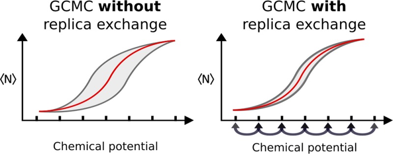
The ability of grand canonical Monte Carlo (GCMC) to create and annihilate molecules in a given region greatly aids the identification of water sites and water binding free energies in protein cavities. However, acceptance rates without the application of biased moves can be low, resulting in large variations in the observed water occupancies. Here, we show that replica-exchange of the chemical potential significantly reduces the variance of the GCMC data. This improvement comes at a negligible increase in computational expense when simulations comprise of runs at different chemical potentials. Replica-exchange GCMC is also found to substantially increase the precision of water binding free energies as calculated with grand canonical integration, which has allowed us to address a missing standard state correction.
Introduction
Aided by community efforts such as the Drug Design Data Resource (D3R) and Statistical Assessment of the Modeling of Proteins and Ligands (SAMPL) challenges,1−3 rigorous binding free energy calculations are becoming increasingly feasible and reliable for use in drug discovery projects.4 Recent studies using these methods have reported promising results in predicting and explaining the selectivity of small molecule inhibitors to protein targets.5,6 In addition to predicting the binding affinity of small molecules to proteins, free energy calculations can also help validate hypotheses in structure-based drug design. In particular, medicinal chemists often seek to exploit the existence of water molecules in binding sites by designing compounds that will displace water upon binding.7,8 While there are a number of cases where the targeted displacement of water molecules has resulted in more potent and/or specific compounds,9−11 there are also examples where new compounds have failed to displace a water molecule,12,13 or in doing so have reduced the affinity of the compound.14,15 Binding free energy calculations using all-atom simulations have the potential to help medicinal chemists in this endeavor, as the calculated binding free energies for water at particular sites have been shown to be indicative of how “displaceable” a water molecule is.16
One of the most popular ways to calculate the absolute binding free energy of water is via double decoupling (DD).17−20 This method uses two sets of simulations that gradually reduce the interaction energy between a chosen water molecule and the rest of the system over a series of nonphysical, alchemical, intermediate states. One simulation alchemically decouples a water molecule from a particular location in a protein and the other decouples a water molecule from bulk solvent. When performing DD calculations on water molecules, the bulk solvent calculation need only be performed once for a given water model and set of simulation parameters (such as the length of the nonbonded cutoff). The decoupling calculations in the protein require the careful application of constraints and/or restraints to keep the water molecule in question bound to a particular location and to prevent other water molecules drifting into the site after decoupling. Applying DD calculations to a bonded network of buried water molecules would require not only cumbersome constraints but also a separate decoupling simulation for each water in the network. The water molecules should be decoupled in the order of weakest to tightest bound, but establishing the correct order will require multiple simulations, and the choice of pathway may increase the variance of the results.
Using binding free energy calculations of water to drive rational drug design is predicated on knowing the probable locations of water within binding sites. While X-ray crystallography is the most well used method of structure determination, locating water sites within X-ray structures is fraught with difficulty. For instance, water molecules may be artifactual,21 may not appear at a given level of resolution,22−24 or may require special techniques to find them.25 There can even be poor agreement between high-resolution structures, with studies finding that an observed water has approximately only a 50% chance of being within 1 Å of an independently resolved structure of the same protein.26,27 Molecular simulations with explicit water offer the possibility of predicting the locations of water in protein cavities that are consistent with the force field used in the free energy calculation. However, despite the ever-increasing time scales accessible by molecular dynamics (MD) simulations—brought about by specialized processors and GPU accelerated code28,29—water molecules that are buried within proteins are systematically under sampled in MD. Nuclear magnetic resonance studies have indicated that the residence times of water in cavities that are inaccessible to bulk water range from tens to hundreds of microseconds,30,31 which is beyond the time scales typically explored by MD studies.
We recently reported theoretical and methodological improvements to the sampling technique known as grand canonical Monte Carlo (GCMC) applied to water.32 In essence, GCMC can be considered as an enhanced sampling method, as molecules (in this case water molecules) can be created and annihilated within a given cavity, circumventing the kinetic barriers that would be encountered in MD and, thus, aiding the determination of water sites. The recent improvements to GCMC allowed for the determination of the absolute binding free energy of highly coupled networks of water as well as the relative stabilities of individual water molecules, all in a single set of simulations. Key to the latest developments in GCMC was the exploitation of simulations performed at a range of different chemical potentials as part of a technique we refer to as grand canonical integration (GCI). When applied to calculating the binding affinity of networks of water molecules, GCI was both easier to execute and computationally less intensive than sequential alchemical DD calculations. However, the statistical uncertainty with GCI was found to be significantly larger than for DD.
Although GCMC sampling of water is orders of magnitude more time efficient than MD in sampling buried sites, GCMC suffers from its own sampling difficulties that affect the precision of the free energy calculations. In GCMC, Metropolis–Hastings acceptance rates for insertions and deletions are low, often <1%.33 This is due to the possibility of steric clashes when inserting molecules into dense systems and large energy deficits when removing waters from systems. An early solution to this issue is the cavity-bias algorithm by Mezei,33 where before every insertion, a random set of points is uniformly sampled within the GCMC simulation region, and an insertion is attempted on a randomly selected point that does not clash with the system. This idea was later developed by Woo et al.,34 who used a dynamically updated grid that kept track of the free space. Orientational biases have also been applied to improve insertion rates.34,35 A recurring issue with such Monte Carlo biasing schemes is whether the increased time of computing and applying a bias does not nullify the improvement in sampling efficiency.
Based on the benefits in sampling seen with temperature,36 Hamiltonian,37−39 and constant pH replica-exchange methods,40 here we apply replica-exchange (RE) to the chemical potential in GCMC simulations. While biasing schemes can suffer from increased computing time as a payoff for their enhanced sampling, the addition of RE to the GCI protocol achieves enhanced sampling with a negligible effect on the run-time. The variance of these calculated free energies significantly decreased with RE, which allowed for comparisons between GCI and double decoupling calculations at a higher level of precision than was previously possible. This facilitated a detailed examination of the GCI binding free energy equation and prompted the development of an improved equation that, unlike before, computes standard state binding free energies. Therefore, the GCMC-based method reported here is more accurate and precise than the previous,32 with a statistical uncertainty that is comparable to double decoupling. Thus, absolute binding free energy calculations with GCI may be an “all in one” solution for water-focused medicinal computational chemistry, as a single set of simulations can determine a large number of properties of the water molecules, pertinently indicating which of the waters, or sets of waters, are most displaceable. GCMC is able to determine locations of water molecules, binding free energies of networks, and cooperativity in a single simulation.
Theory
Grand Canonical Monte Carlo
GCMC is the technique that allows for the creation and annihilation of molecules within a simulation. By construction, simulation statistics in GCMC are consistent with the grand canonical ensemble, where it is imagined that the system of interest can exchange molecules with a reservoir. The reservoir exists in a predetermined thermodynamic state that is specified by its temperature and chemical potential, which accounts for the average density and interaction energy of the molecular species in the reservoir. This work is concerned with performing GCMC on water molecules within protein cavities, such that the natural choice of the reservoir is bulk water at room temperature.
In Adams’s formulation of GCMC,41 the probability to insert one molecule into the simulated system from the reservoir is given by
| 1 |
and the probability to remove one molecule from the system and add it to the reservoir is given by
| 2 |
where N is the instantaneous number of molecules of the chemical species in the system, ΔE is the change in potential energy of inserting or removing the water molecule, β is the inverse temperature, and B is the applied Adams parameter,41 a term that accounts for the chemical potential of the reservoir and the volume of the simulated system. Originally defined by Adams in terms of the excess chemical potential and average occupancy of the system,41B is related to the applied chemical potential, μ, and volume of the GCMC region, V, via
| 3 |
where Λ3 is the thermal wavelength of the GCMC molecule.
Replica-Exchange GCMC
Guarnieri and Mezei pioneered the technique in which many independent GCMC simulations of water are performed at a range of different B values—equivalently, different chemical potentials.42 By viewing how and where the occupancy of water changed as a function of B, they obtained a semiquantitative map of the regions of high water affinity. By analogy with ligand-protein binding assays, we use the term “titration” to refer to a set of GCMC simulations of the same system at different B values. This titration technique was extended in our previous study where the average number of water molecules as a function of B could be integrated to predict the binding free energies of water networks.32 This method is referred to as GCI and is discussed in more detail below. Given the utility of performing GCMC simulations at different chemical potentials, and the sampling improvements gained by Hamiltonian RE in alchemical free energy calculations,37,38 RE of the B values in GCMC simulations has the potential to improve the accuracy of the free energies calculated with GCI.
When running concurrent GCMC simulations at a range of chemical potentials, the probability of accepting a Metropolis–Hastings move that swaps the B values of the ith and jth simulations is given by
| 4 |
where Ni and Nj are the number of water molecules in the ith and jth replicas. This equation is similar to the Metropolis–Hastings criteria in constant-pH RE40 as well as parallel tempering and Hamiltonian RE36 and is derived in the Supporting Information (SI) by constructing an expanded ensemble that allows for chemical potentials to vary. One would expect RE of the chemical potentials to enhance the sampling in GCMC titrations, because simulations at high chemical potentials, where insertions are more likely, can mix with simulations at low chemical potentials, where deletions are more likely.
Binding Free Energies with Grand Canonical Integration
GCI is a technique that integrates over the average number of water molecules as a function of the B value to predict the relative binding free energies of water molecules.32 If at the lowest B value there are no waters bound, then GCI can predict absolute binding free energies. When applied to calculating the binding free energy of water networks, the GCI method is more computationally efficient and easier to implement than traditional double-decoupling techniques,32 which require multiple simulations for each water molecule in the network as well as the careful application of restraints or constraints.
Given that GCI uses the information from simulations run at different B values, one can expect the statistical uncertainty of the calculated free energies to improve with RE. Indeed, as shown in the Results section and SI, the gain in precision afforded by RE revealed that binding free energies calculated with the method described previously32 were dependent on the volume of the GCMC region and had statistically resolvable systematic differences with free energies calculated by double decoupling. This prompted a re-examination of the equation used to calculate binding free energies with GCI. While the original GCI equation—for the free energy to transfer water from ideal gas to the system of interest at a fixed volume—is correct, the standard state corrections were missing for the binding free energy. Derived in the SI, the equation to calculate relative standard state binding free energies between an initial average number of waters Ni and final average number Nf is given by
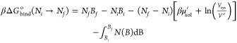 |
5 |
where Bk is the Adams parameter for which there are an average of Nk waters, Vsys is the volume of the GCMC region, Vo is the standard state volume of bulk water, and μsol′ is the excess chemical potential of the water in bulk water. For practical purposes, μsol is the hydration free energy of the simulated water model.
In contrast to the previous binding energy equation, this has a term for the volume of the GCMC region, and no longer depends on the factorial of Ni and Nf. As shown in the SI, these changes come from removing the implicit assumption in the previous derivation that both the free energies of the simulated system and reservoir had the same contribution from the ideal gas.
In addition to the theoretical derivation, the effect of the volume term of the GCI equation on the calculated binding free energies has been empirically tested using a very well converged, idealized protein-ligand system based on scytalone dehydratase. The binding free energies of water molecules should be independent of the size of the GCMC subvolume, and these results demonstrate this. These results are available in the SI and confirm that eq 5 is the correct form of the GCI equation.
The new GCI equation is also consistent with the following equilibrium condition for water binding:
| 6 |
where μsys is the chemical potential for water in the simulated system, and μsol is the chemical potential for water in bulk solvent. This relation is also derived in the SI. Owing to the previous implicit assumption about the ideal gas contribution to the free energies, this was previously erroneously stated as the equality of excess chemical potentials.32Eq 6 makes it straightforward to set the B value for a GCMC simulation where water molecules in the system of interest are in equilibrium with bulk water:
| 7 |
Given that the hydration free energy and density of bulk water only need to be calculated once per water model, one can set the Adams parameter, or chemical potential, prior to running a GCMC simulation, where equilibrium with bulk water is desired.
Methods
Simulations were performed to (1) assess whether RE of B values in GCMC titration simulations (RE-GCMC) improves the consistency and accuracy of repeated GCMC simulations and free energies calculated with GCI and (2) determine the degree of precision with which the new GCMC methodology agrees with double decoupling in biomolecular systems. The protein system bovine pancreatic trypsin inhibitor (BPTI) was used to address these aims, chosen due to its prior use as a model system.43
BPTI was used to test the ability of RE-GCMC to improve the sampling of GCMC titration simulations and to compare free energies calculated with GCI and RE to estimates from double decoupling. All simulations focused on a small cavity in BPTI that binds to three water molecules. In our previous investigations,32 this system was found to be the worst sampled of all 10 systems studied and thus will most clearly highlight any improvements over the previous methodology. The simulated structure was taken from protein data bank (PDB) entry 5PTI and was prepared as previously described.32 The protein backbone and side chain atoms were sampled over the angles and dihedrals. Backbone moves within ProtoMS are performed by rigid-body translations and rotations, centered on the intersection of the Cα–N, and C=O bond vectors. The structure was solvated inside a half-harmonically restrained, spherical droplet of water, with a radius chosen such that the edge of the droplet was approximately 15 Å away from the surface of the protein.
All simulations were performed with the freely available Monte Carlo simulation package ProtoMS, version 3.3.44 The TIP4P water model45 and the AMBER14SB force-field46 were used. Nonbonded interactions were truncated, using a residue-based switching cutoff, at 10 Å.
GCMC
In ProtoMS, GCMC insertion and deletion moves are only made inside a user-defined, cuboidal subvolume of the system. Once inserted, water molecules can translate and rotate. Insertion, deletion, and translation/rotation moves for GCMC are attempted with equal probability. To keep track of the number of waters inside the GCMC subvolume, a hard-wall constraint is applied to inserted water molecules to prevent them from drifting away, and bulk solvent water molecules are not allowed to enter from outside the subvolume.
Water molecules were inserted and deleted within the box over the three-water cavity shown in Figure 1. The box had dimensions 5.0 × 4.0 × 8.0 Å3 and an origin of (29.0, 5.0, −2.0) Å in the reference frame of the PDB structure. Titration simulations were run with integer B values between −31.0 and 0.0, inclusive. For equilibration, 1 million (M) GCMC-only moves were performed with the rest of the system fixed, followed by 1 M moves of GCMC and protein and solvent configuration sampling, where each repeat was equilibrated independently. The production simulations comprised 10 repeats of 100 M moves. When fully sampling the whole system, protein, bulk solvent, and grand canonical insertion, deletion, and translation/rotation sampling were trialled with the ratios 461:39:167:167:167, respectively.
Figure 1.
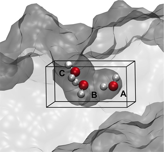
Cavity in the BPTI protein, with waters A, B, and C bound. The surface of the protein is shown with a transparent gray surface. The GCMC box covering the water sites is delineated with black lines.
To assess the impact of RE on the consistency of the GCMC results, simulations were performed without RE and with RE with B value exchanges attempted with randomly selected nearest neighbors every 100,000, 200,000, 500,000, and 1 M MC moves.
Double Decoupling
For each water location found with GCMC, decoupling simulations were performed to determine the binding free energy of each water. Decoupling was performed over 16 alchemical λ states, where the Lennard-Jones and Coulombic terms were scaled simultaneously. Moves were split between protein, bulk water, and decoupled water at a ratio of 402:98:1 respectively. The water molecules were decoupled sequentially, from weakest to strongest bound. Where the free energies of multiple waters are similar, calculations were repeated with a different order of decouplings. 500,000 equilibration and 40 M production moves were performed for each water at each λ value. Each simulation was repeated four times. Soft-cores (soft66 in ProtoMS package)47−49 were used for decoupling calculation with δ = 0.2 and δc = 2.0. The free energy to decouple the water from the system was determined using MBAR.50
A harmonic restraint with a force constant of 2 kcal mol–1 Å–2 was used on the oxygen of the water being decoupled at all λ values. A gas phase correction of
| 8 |
where
| 9 |
was applied to account for the removal of the restraint from the decoupled system.51 This is analogous to the volume term introduced in the GCI equation, eq 5. Prompted by the higher precision obtained in RE-GCMC and unlike our previous study,32 the free energy penalty of applying the harmonic restraint in the bound simulation was calculated using Bennett’s acceptance ratio method from 40,000 Monte Carlo simulation steps with six equally spaced λ values of the restraint from 0 kcal mol–1 Å–2 to 2 kcal mol–1 Å–2. No symmetry correction was applied to water molecules. More details on the location of the restraints and the resulting free energy corrections are available in the SI.
Results
Replica-Exchange with BPTI
GCMC calculations were performed on BPTI with and without RE in B. The titration results from 10 repeats with no RE and the most frequent RE (attempted every 100,000 MC steps) are shown in Figure 2. The acceptance rate for the attempted exchanges between B replicas was >89% for all RE frequencies. More details of this are available in the SI.
Figure 2.

Ten repeats of GCMC titration data for the BPTI system, without RE (left) in B and RE every 100,000 steps (right). Each point corresponds to the average number of water molecules at a given B value. The first 200,000 MC steps have been excluded as equilibration.
Figure 2 shows that RE has improved the repeatability of the titration data. The Kolmogorov–Smirnov52 test was used to test the statistical significance of this apparent reduction in uncertainty. All values of N from simulations with and without RE were median centered to focus only on the spread of the Ns and not the relationship with B. The distributions of median-centered N with and without RE were found to be significantly different with a p-value of 0.0135. The relationship between B and N should be monotonically increasing owing to the relationship between B value and average water occupancy (see eqs 1 and 2). The monotonicity of each individual titration repeat, therefore, provides an additional quantifiable test of sampling performance. The Kendall rank correlation coefficient, denoted τ, is an appropriate measure of the montonicity as it does not require a linear relationship between B and N. A perfect monotonically increasing relationship between B and N is indicated by τ = 1. The mean τ with one standard error for the non-RE titration data is 0.86 ± 0.01, compared to 0.98 ± 0.00 for RE-GCMC, averaged over all RE frequencies. Hence, the titration data from RE-GCMC are more physically sound than without RE.
Using eq 5, the titration data for all the BPTI simulations were used to calculate binding free energies for each RE frequency. As the purpose is to evaluate the extent to which the uncertainty in the GCI free energy decreases with RE, Figure 3 shows the boxplots of the median-centered binding free energy for one, two, and three waters, whose locations can be seen in Figure 1. The boxplots were generated by bootstrap sampling the titration data and calculating the GCI binding free energy of each sample. A bootstrap sample consisted of one randomly sampled N value from the set of 10 repeats for each of the 32 B values, and the titration curve was estimated as previously described.32 Both the interquartile ranges and the range of the data (illustrated by the “whiskers”) are larger for the protocols with no RE. The statistical significance of this reduction in spread with RE was assessed using the bootstrap samples of the free energy to bind three waters. The variance of the binding free energy was calculated in batches of 10 bootstrap samples for all RE data and separately for free energies calculated without RE. Using these samples, we estimate that the probability that the variance with RE is equal to or greater than the variance without RE to be 2.6%. Thus, the reduction in the variance of calculated free energies is statistically significant. This result is consistent both with the increased monotonicity and the reduced titration variance found for RE-GCMC. Therefore, RE-GCMC improves the repeatability of individual titration simulations. There is no clear RE frequency that is significantly better than the rest (see Figure S5).
Figure 3.
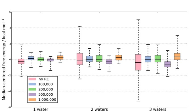
Boxplot of the median-centered free energies for each protocol, where errors have been calculated over 1000 bootstrapping steps of 10 repeats. In each case it is the free energy difference between an empty GCMC region, to a one, two and three water network, respectively. RE with GCI produces free energies that have a consistently tighter distribution than GCI free energies calculated without RE.
Figure 4 compares the binding free energies calculated for the three-water BPTI network using GCI and double decoupling. The standard deviation over the repeats is used to illustrate the relative uncertainty of each method. The distribution of the error of original GCI binding free energy equation32 without RE overlaps with the distribution of error with the new standard state formulation (eq 5) and double decoupling. With the benefit of the higher precision granted by RE, the standard state binding free energy formulation of GCI is more clearly in agreement with the standard state binding free energies as calculated via double decoupling. Indeed, the standard deviation of GCI is comparable to, if not smaller than, double decoupling. In addition to this, the GCI method is easier to use than double decoupling, as all of the water binding free energies are determined in a single, automated set of simulations. GCMC does not require the a priori knowledge of both the number of waters and the location of the waters that are needed for double decoupling simulations. Double decoupling methods also require restraints or constraints within the simulations. Both restraints and constraints are needed to reduce the sampling of the water molecule as it is decoupled from the system, but constraints are also able to prevent other nearby water molecules occupying the site. GCMC is a significantly easier method to implement and, with the addition of RE, is able to provide results with comparable variance.
Figure 4.
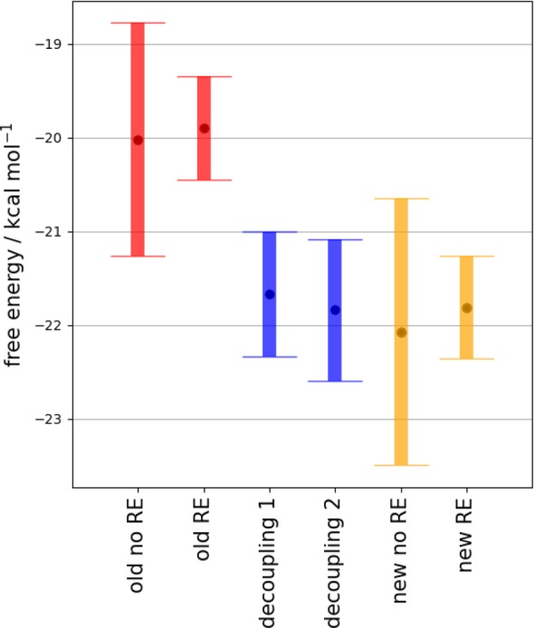
Binding free energies of the three water network in BPTI calculated using different methods. To highlight the intrinsic uncertainty of each method, the colored bars indicate the standard deviation, as opposed to the standard error, over all repeats. Blue results are from sequential decoupling of the water network, with decoupling 1 waters are decoupled in the order C–B–A and decoupling 2 in the order C–A–B. Red results show the binding free energies calculated with the orginal formulation of GCI binding free energy equation for both RE (frequency: 100,000) and non-RE simulations, and the orange results are from the same simulations determined using eq 5.
The detailed breakdown of the BPTI thermodynamic cycle is shown in Figure 5. The binding free energies of the water molecules in the BPTI system were determined by decoupling calculations. As Figure 2 shows, two water molecules appear to couple into the BPTI system simultaneously (waters A and B), followed by a third molecule at a higher chemical potential (water C). As waters A and B couple in simultaneously, the decoupling of these water molecules has been attempted in both orders (i.e., A then B, and B then A) with double decoupling. The results are shown in Figure 5, and the closures of the thermodynamic cycles (shown in red) are consistent to within error. The free energy of the three water network is −21.81 (0.50), −21.67 (0.68), and −21.84 (0.74) kcal mol–1 as calculated by GCI with RE-GCMC and the two double decoupling pathways, respectively. As GCI couples the first two waters in simultaneously, it is not possible to decompose the free energy of the dimer to free energies for separate waters. The GCI simulations were analyzed to look at all of the simulation snapshots across all B values for structures where only one water is present in the site of interest, and in the majority of cases, water B is present more often than water A, suggesting that it is the first to couple into the system, albeit with similar free energies of binding. Performing the double decoupling simulation, as water B has a larger binding free energy when coupling the dry cavity than water A (−8.20 kcal mol–1 and −5.85 kcal mol–1), respectively, double decoupling suggests that water B will enter the protein system first. The largest error between GCI and double decoupling occurs in the leg with the order of water B then water A. The largest error of the cycle is the decoupling leg of water B to a dry cavity, where the standard error of calculations is 0.63.
Figure 5.
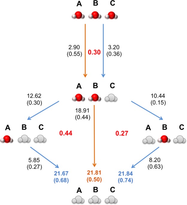
Thermodynamic cycle of BPTI. Orange arrows, GCMC results; blue arrows, decoupling results. GCMC values are calculated using a RE frequency of 100,000. Standard errors are shown in parentheses. Gray waters indicate which waters have been turned “off” in the system. Cycle closure energies are shown in bold red. All values are recorded in kcal mol–1.
Discussion and Conclusions
This work has used replica-exchange (RE) of the chemical potential (equivalently, Adams parameter) in grand canonical Monte Carlo (GCMC) to calculate the absolute binding free energies of small networks of water molecules to protein cavities. The use of RE was found to significantly reduce the variance of the water occupancies at each applied chemical potential, which resulted in a significant reduction in variances of the absolute binding free energies as calculated with grand canonical integration (GCI). The decreased variance of the GCMC simulations facilitated the precise comparison of water binding free energies calculated using double decoupling and the standard state GCI binding free energy equation developed herein. The free energies calculated from both methods were found to be in agreement.
In this study, the absolute binding free energies calculated from GCMC (using GCI) have lower statistical uncertainties than the free energies calculated via alchemical decoupling (estimated using MBAR). This difference becomes more pronounced the more water molecules are decoupled in spite of the fact that, in our hands, free energy calculations with GCMC require fewer CPU hours than alchemical decoupling in BPTI and simpler applications of constraints/restraints. For binding free energy calculations with greater numbers of water molecules, we expect the gap between accuracy and performance to widen between GCMC and alchemical methods.
The extent to which the precision and speed of the GCMC binding free energy methods carries over from water molecules to small, drug-like molecules remains to be seen. The use of GCMC with unbiased insertion moves, as used here for water, becomes increasingly inefficient for larger molecules due to higher probabilities of steric clashes. Nevertheless, GCMC has already been successfully applied to small fragments, both with unbiased insertion moves53 and using cavity bias.54 The techniques developed here, therefore, may hold promise for the rigorous calculation of absolute binding free energies of small fragments via GCMC. Larger molecules will no doubt require the application of configurational biasing techniques,33,35,55 although these do come with the additional computational effort required to compute the bias. The use of RE for absolute free energy calculations with GCI comes with a negligible increase in the computational burden, as the exchange of information across CPU nodes is orders of magnitude faster than the run-time of the molecular simulation.
A curious feature of GCMC simulations is the requirement that the volume must remain constant. This is so that the simulations correctly sample the grand canonical (μVT) ensemble. As protein-ligand binding affinities are typically measured under constant pressure conditions, a natural question is to what extent GCMC-like techniques can be used in constant-pressure simulations, such as those in the isothermal-isobaric (NpT) ensemble. Despite the fact that the NpT-type ensembles require the number of particles to remain constant, there are a number of Markov chain Monte Carlo techniques that have insertion and deletion moves, in addition to volume moves, as part of their sampling repertoire. For instance, the Gibbs-ensemble Monte Carlo method56,57 attempts to replicate the physically impossible μpT ensemble by allowing two simulated compartments to exchange volume and molecules or particles. Although the volume and number of particles in either compartment can fluctuate, the combined volume and the total number of particles must remain constant. Other techniques employ the semigrand canonical ensemble (see, for example, refs (58 or 59)), in which the composition of the system can change (i.e., allowing different fragments to interconvert) under the constraint that the total number of particles remains constant. The semigrand canonical ensemble also requires the difference in the chemical potentials of the interconverting molecules to remain constant so that, when there are only two interconverting molecular species, the semigrand canonical ensemble can be described as a NpTΔμ ensemble. In controlling the ratio of two species, the Δμ parameter operates—in practice—very much like the μ parameter in GCMC, so that semigrand canonical simulations are amenable to enhanced sampling via the RE method described herein.
Absolute binding free energy calculations with GCMC can calculate both the location and binding free energy of networks of waters as well as the relative stability of the individual waters. The methods developed here reduce both the bias and variance of the predictions made with GCI compared to its original implementation. Coupled with its ease of use compared to double decoupling, we hope GCI will be a powerful tool in structure-based design, particularly in cases where one seeks to rigorously quantify the effect of structural waters on ligand binding affinities.
Acknowledgments
The authors thank the EPSRC and NIH for funding. G.A.R. is supported by the Memorial Sloan Kettering Cancer Center, NIH grant P30 CA008748 and EPSRC grant EP/J010189/1. H.B.M. is supported by the EPSRC funded CDT in Theory and Modelling in Chemical Sciences, under grant EP/L015722/1. C.C.-A. is supported by an EPSRC Doctoral Training Centre grant EP/G03690X/1. J.W.E. holds a Royal Society Wolfson Research Merit Award. We acknowledge iSolution at the University of Southampton for computing time on the Iridis4 cluster.
Supporting Information Available
The Supporting Information is available free of charge on the ACS Publications website at DOI: 10.1021/acs.jctc.7b00738.
Derivation of the RE criterion (eq 4), derivation of standard state grand canonical integration binding free energy expression (eq 5), and derivation of the equilibrium condition in eq 6. Further investigation and analysis of the new standard state grand canonical integration equation was carried out on scytalone dehydratase test systems with the methods and results fully described. The data show how the standard state binding free energy equation does not depend on the volume of the GCMC region as expected, and that the calculated free energies agree with double decoupling calculations to a high degree of precision. Additional information is also provided on the methods, analysis, and results of the bovine pancreatic trypsin inhibitor simulations. This information includes the acceptance rates for GCMC insertion and deletion moves, acceptance rates for RE moves, the degree to which RE reduces the variance of estimated water occupancies, as well as details on the GCMC subvolumes and double decoupling restraints that were used (PDF)
The authors declare no competing financial interest.
Supplementary Material
References
- Gathiaka S.; Liu S.; Chiu M.; Yang H.; Stuckey J.; Kang Y.; Delproposto J.; Kubish G.; Dunbar J.; Carlson H.; Burley S.; Walters; Amaro R.; Feher V.; Gilson M. D3R grand challenge 2015: Evaluation of protein-ligand pose and affinity predictions. J. Comput.-Aided Mol. Des. 2016, 30, 651–668. 10.1007/s10822-016-9946-8. [DOI] [PMC free article] [PubMed] [Google Scholar]
- Yin J.; Henriksen N.; Slochower D.; Shirts M.; Chiu M.; Mobley D.; Gilson M. Overview of the SAMPL5 host-guest challenge: Are we doing better?. J. Comput.-Aided Mol. Des. 2017, 31, 1–19. 10.1007/s10822-016-9974-4. [DOI] [PMC free article] [PubMed] [Google Scholar]
- Mikulskis P.; Cioloboc D.; Andrejić M.; Khare S.; Brorsson J.; Genheden S.; Mata R.; Söderhjelm P.; Ryde U. Free-energy perturbation and quantum mechanical study of SAMPL4 octa-acid host-guest binding energies. J. Comput.-Aided Mol. Des. 2014, 28, 375–400. 10.1007/s10822-014-9739-x. [DOI] [PubMed] [Google Scholar]
- Michel J.; Foloppe N.; Essex J. W. Rigorous Free Energy Calculations in Structure-Based Drug Design. Mol. Inf. 2010, 29, 570–578. 10.1002/minf.201000051. [DOI] [PubMed] [Google Scholar]
- Lin Y.-L.; Meng Y.; Huang L.; Roux B. Computational Study of Gleevec and G6G Reveals Molecular Determinants of Kinase Inhibitor Selectivity. J. Am. Chem. Soc. 2014, 136, 14753–14762. 10.1021/ja504146x. [DOI] [PMC free article] [PubMed] [Google Scholar]
- Aldeghi M.; Heifetz A.; Bodkin M. J.; Knapp S.; Biggin P. C. Predictions of Ligand Selectivity from Absolute Binding Free Energy Calculations. J. Am. Chem. Soc. 2017, 139, 946–957. 10.1021/jacs.6b11467. [DOI] [PMC free article] [PubMed] [Google Scholar]
- Bissantz C.; Kuhn B.; Stahl M. A Medicinal Chemist’s Guide to Molecular Interactions. J. Med. Chem. 2010, 53, 5061–5084. 10.1021/jm100112j. [DOI] [PMC free article] [PubMed] [Google Scholar]
- Huggins D. J.; Sherman W.; Tidor B. Rational Approaches to Improving Selectivity in Drug Design. J. Med. Chem. 2012, 55, 1424–1444. 10.1021/jm2010332. [DOI] [PMC free article] [PubMed] [Google Scholar]
- Lam P. Y.; Jadhav P. K.; Eyermann C. J.; Hodge C. N.; Ru Y.; Bacheler L. T.; Meek J. L.; Otto M. J.; Rayner M. M.; Wong Y. N. Rational Design of Potent, Bioavailable, Nonpeptide Cyclic Ureas as HIV Protease Inhibitors. Science 1994, 263, 380–384. 10.1126/science.8278812. [DOI] [PubMed] [Google Scholar]
- Chen J. M.; Xu S. L.; Wawrzak Z.; Basarab G. S.; Jordan D. B. Structure-Based Design of Potent Inhibitors of Scytalone Dehydratase: Displacement of a Water Molecule from the Active Site. Biochemistry 1998, 37, 17735–17744. 10.1021/bi981848r. [DOI] [PubMed] [Google Scholar]
- Biela A.; Sielaff F.; Terwesten F.; Heine A.; Steinmetzer T.; Klebe G. Ligand Binding Stepwise Disrupts Water Network in Thrombin: Enthalpic and Entropic Changes Reveal Classical Hydrophobic Effect. J. Med. Chem. 2012, 55, 6094. 10.1021/jm300337q. [DOI] [PubMed] [Google Scholar]
- Vollmuth F.; Geyer M. Interaction of Propionylated and Butyrylated Histone H3 Lysine Marks with Brd4 Bromodomains. Angew. Chem., Int. Ed. 2010, 49, 6768–6772. 10.1002/anie.201002724. [DOI] [PubMed] [Google Scholar]
- Kadirvelraj R.; Foley B. L.; Dyekjær J. D.; Woods R. J. Involvement of Water in Carbohydrate-Protein Binding: Concanavalin A Revisited. J. Am. Chem. Soc. 2008, 130, 16933–16942. 10.1021/ja8039663. [DOI] [PMC free article] [PubMed] [Google Scholar]
- Mikol V.; Papageorgiou C.; Borer X. The Role of Water Molecules in the Structure-Based Design of (5-Hydroxynorvaline)-2-cyclosporin: Synthesis, Biological Activity, and Crystallographic Analysis with Cyclophilin A. J. Med. Chem. 1995, 38, 3361–3367. 10.1021/jm00017a020. [DOI] [PubMed] [Google Scholar]
- Nasief N. N.; Tan H.; Kong J.; Hangauer D. Water Mediated Ligand Functional Group Cooperativity: The Contribution of a Methyl Group to Binding Affinity is Enhanced by a COO- Group Through Changes in the Structure and Thermodynamics of the Hydration Waters of Ligand-Thermolysin Complexes. J. Med. Chem. 2012, 55, 8283–8302. 10.1021/jm300472k. [DOI] [PMC free article] [PubMed] [Google Scholar]
- Barillari C.; Taylor J.; Viner R.; Essex J. W. Classification of Water Molecules in Protein Binding Sites. J. Am. Chem. Soc. 2007, 129, 2577–2587. 10.1021/ja066980q. [DOI] [PubMed] [Google Scholar]
- Hamelberg D.; McCammon J. A. Standard Free Energy of Releasing a Localized Water Molecule from the Binding Pockets of Proteins: Double-Decoupling Method. J. Am. Chem. Soc. 2004, 126, 7683–7689. 10.1021/ja0377908. [DOI] [PubMed] [Google Scholar]
- García-Sosa A. T.; Mancera R. L. Free Energy Calculations of Mutations Involving a Tightly Bound Water Molecule and Ligand Substitutions in a Ligand-Protein Complex. Mol. Inf. 2010, 29, 589–600. 10.1002/minf.201000007. [DOI] [PubMed] [Google Scholar]
- Michel J.; Tirado-Rives J.; Jorgensen W. L. Energetics of Displacing Water Molecules from Protein Binding Sites: Consequences for Ligand Optimization. J. Am. Chem. Soc. 2009, 131, 15403–15411. 10.1021/ja906058w. [DOI] [PMC free article] [PubMed] [Google Scholar]
- Bodnarchuk M. S.; Viner R.; Michel J.; Essex J. W. Strategies to Calculate Water Binding Free Energies in Protein-Ligand Complexes. J. Chem. Inf. Model. 2014, 54, 1623–1633. 10.1021/ci400674k. [DOI] [PubMed] [Google Scholar]
- Davis A. M.; Teague S. J.; Kleywegt G. J. Application and Limitations of X-ray Crystallographic Data in Structure-based Ligand and Drug Design. Angew. Chem., Int. Ed. 2003, 42, 2718–2736. 10.1002/anie.200200539. [DOI] [PubMed] [Google Scholar]
- Carugo O.; Bordo D. How Many Water Molecules can be Detected by Protein Crystallography?. Acta Crystallogr., Sect. D: Biol. Crystallogr. 1999, 55, 479–483. 10.1107/S0907444998012086. [DOI] [PubMed] [Google Scholar]
- Wlodawer A.; Minor W.; Dauter Z.; Jaskolski M. Protein Crystallography for Non-crystallographers, or how to get the Best (but not More) from Published Macromolecular Structures. FEBS J. 2008, 275, 1–21. 10.1111/j.1742-4658.2007.06178.x. [DOI] [PMC free article] [PubMed] [Google Scholar]
- Nittinger E.; Schneider N.; Lange G.; Rarey M. Evidence of Water Molecules - A Statistical Evaluation of Water Molecules Based on Electron Density. J. Chem. Inf. Model. 2015, 55, 771–783. 10.1021/ci500662d. [DOI] [PubMed] [Google Scholar]
- Yu B.; Blaber M.; Gronenborn A. M.; Clore G. M.; Caspar D. L. D. Disordered Water Within a Hydrophobic Protein Cavity Visualized by X-ray Crystallography. Proc. Natl. Acad. Sci. U. S. A. 1999, 96, 103–108. 10.1073/pnas.96.1.103. [DOI] [PMC free article] [PubMed] [Google Scholar]
- Nucci N. V.; Pometun M. S.; Wand A. J. Site-resolved Measurement of Water-Protein Interactions by Solution NMR. Nat. Struct. Mol. Biol. 2011, 18, 245–249. 10.1038/nsmb.1955. [DOI] [PMC free article] [PubMed] [Google Scholar]
- Ross G. A.; Morris G. M.; Biggin P. C. Rapid and Accurate Prediction and Scoring of Water Molecules in Protein Binding Sites. PLoS One 2012, 7, e32036. 10.1371/journal.pone.0032036. [DOI] [PMC free article] [PubMed] [Google Scholar]
- Shaw D. E.et al. Anton 2: Raising the Bar for Performance and Programmability in a Special-Purpose Molecular Dynamics Supercomputer. Proceedings from the SC14: International Conference for High Performance Computing, Networking, Storage and Analysis, New Orleans, LA, November 16–21, 2014; IEEE: Piscataway, NJ, 2014; pp 41–53.
- Stone J. E.; Hardy D. J.; Ufimtsev I. S.; Schulten K. GPU-accelerated Molecular Modeling Coming of Age. J. Mol. Graphics Model. 2010, 29, 116–125. 10.1016/j.jmgm.2010.06.010. [DOI] [PMC free article] [PubMed] [Google Scholar]
- Denisov V. P.; Halle B.; Peters J.; Hörlein H. D. Residence Times of the Buried Water Molecules in Bovine Pancreatic Trypsin Inhibitor and its G36S Mutant. Biochemistry 1995, 34, 9046–9051. 10.1021/bi00028a013. [DOI] [PubMed] [Google Scholar]
- Ernst J. A.; Clubb R. T.; Zhou H. X.; Gronenborn A. M.; Clore G. M. Demonstration of Positionally Disordered Water Within a Protein Hydrophobic Cavity by NMR. Science 1995, 267, 1813–1817. 10.1126/science.7892604. [DOI] [PubMed] [Google Scholar]
- Ross G. A.; Bodnarchuk M. S.; Essex J. W. Water Sites, Networks, And Free Energies with Grand Canonical Monte Carlo. J. Am. Chem. Soc. 2015, 137, 14930–14943. 10.1021/jacs.5b07940. [DOI] [PubMed] [Google Scholar]
- Mezei M. A cavity-biased (T, V, μ) Monte Carlo Method for the Computer Simulation of Fluids. Mol. Phys. 1980, 40, 901–906. 10.1080/00268978000101971. [DOI] [Google Scholar]
- Woo H.-J.; Dinner A. R.; Roux B. Grand canonical Monte Carlo Simulations of Water in Protein Environments. J. Chem. Phys. 2004, 121, 6392–6400. 10.1063/1.1784436. [DOI] [PubMed] [Google Scholar]
- Shelley J. C.; Patey G. N. A configuration bias Monte Carlo method for water. J. Chem. Phys. 1995, 102, 7656–7663. 10.1063/1.469017. [DOI] [Google Scholar]
- Earl D. J.; Deem M. W. Parallel tempering: Theory, Applications, and New Perspectives. Phys. Chem. Chem. Phys. 2005, 7, 3910–3916. 10.1039/b509983h. [DOI] [PubMed] [Google Scholar]
- Sugita Y.; Kitao A.; Okamoto Y. Multidimensional Replica-Exchange Method for Free-Energy Calculations. J. Chem. Phys. 2000, 113, 6042–6051. 10.1063/1.1308516. [DOI] [Google Scholar]
- Woods C. J.; Essex J. W.; King M. A. The Development of Replica-Exchange-Based Free-Energy Methods. J. Phys. Chem. B 2003, 107, 13703–13710. 10.1021/jp0356620. [DOI] [Google Scholar]
- Woods C. J.; Essex J. W.; King M. A. Enhanced Configurational Sampling in Binding Free-Energy Calculations. J. Phys. Chem. B 2003, 107, 13711–13718. 10.1021/jp036162+. [DOI] [Google Scholar]
- Itoh S. G.; Damjanović A.; Brooks B. R. pH Replica-Exchange Method Based on Discrete Protonation States. Proteins: Struct., Funct., Genet. 2011, 79, 3420–3436. 10.1002/prot.23176. [DOI] [PMC free article] [PubMed] [Google Scholar]
- Adams D. J. Chemical Potential of Hard-Sphere Fluids by Monte Carlo Methods. Mol. Phys. 1974, 28, 1241–1252. 10.1080/00268977400102551. [DOI] [Google Scholar]
- Guarnieri F.; Mezei M. Simulated Annealing of Chemical Potential: A General Procedure for Locating Bound Waters. Application to the Study of the Differential Hydration Propensities of the Major and Minor Grooves of DNA. J. Am. Chem. Soc. 1996, 118, 8493–8494. 10.1021/ja961482a. [DOI] [Google Scholar]
- Olano L. R.; Rick S. W. Hydration Free Energies and Entropies for Water in Protein Interiors. J. Am. Chem. Soc. 2004, 126, 7991–8000. 10.1021/ja049701c. [DOI] [PubMed] [Google Scholar]
- Bodnarchuk M.; Bradshaw R.; Cave-Ayland C.; Genheden S.; Cabedo-Martinez A.; Michel J.; Ross G.; Woods C.. ProtoMS; University of Southampton: Highfield, Southampton, 2017; protoms.org.
- Jorgensen W. L.; Chandrasekhar J.; Madura J. D.; Impey R. W.; Klein M. L. Comparison of Simple Potential Functions for Simulating Liquid Water. J. Chem. Phys. 1983, 79, 926–935. 10.1063/1.445869. [DOI] [Google Scholar]
- Maier J. A.; Martinez C.; Kasavajhala K.; Wickstrom L.; Hauser K. E.; Simmerling C. ff14SB: Improving the Accuracy of Protein Side Chain and Backbone Parameters from ff99SB. J. Chem. Theory Comput. 2015, 11, 3696–3713. 10.1021/acs.jctc.5b00255. [DOI] [PMC free article] [PubMed] [Google Scholar]
- Özal T. A.; Peter C.; Hess B.; van der Vegt N. F. A. Modeling Solubilities of Additives in Polymer Microstructures: Single-Step Perturbation Method Based on a Soft-Cavity Reference State. Macromolecules 2008, 41, 5055–5061. 10.1021/ma702329q. [DOI] [Google Scholar]
- Steinbrecher T.; Mobley D. L.; Case D. A. Nonlinear Scaling Schemes for Lennard-Jones Interactions in Free Energy Calculations. J. Chem. Phys. 2007, 127, 214108. 10.1063/1.2799191. [DOI] [PubMed] [Google Scholar]
- Steinbrecher T.; Joung I.; Case D. A. Soft-core Potentials in Thermodynamic Integration: Comparing One- and Two-step Transformations. J. Comput. Chem. 2011, 32, 3253–3263. 10.1002/jcc.21909. [DOI] [PMC free article] [PubMed] [Google Scholar]
- Shirts M. R.; Chodera J. D. Statistically Optimal Analysis of Samples from Multiple Equilibrium States. J. Chem. Phys. 2008, 129, 124105. 10.1063/1.2978177. [DOI] [PMC free article] [PubMed] [Google Scholar]
- Gilson M. K.; Given J. A.; Bush B. L.; McCammon J. A. The Statistical-Thermodynamic Basis for Computation of Binding Affinities: A Critical Review. Biophys. J. 1997, 72, 1047–1069. 10.1016/S0006-3495(97)78756-3. [DOI] [PMC free article] [PubMed] [Google Scholar]
- Smirnov N. Table for Estimating the Goodness of Fit of Empirical Distributions. Ann. Math. Stat. 1948, 19, 279–281. 10.1214/aoms/1177730256. [DOI] [Google Scholar]
- Lakkaraju S. K.; Raman E. P.; Yu W.; MacKerell A. D. Sampling of Organic Solutes in Aqueous and Heterogeneous Environments Using Oscillating Excess Chemical Potentials in Grand Canonical-like Monte Carlo-Molecular Dynamics Simulations. J. Chem. Theory Comput. 2014, 10, 2281–2290. 10.1021/ct500201y. [DOI] [PMC free article] [PubMed] [Google Scholar]
- Clark M.; Guarnieri F.; Shkurko I.; Wiseman J. Grand Canonical Monte Carlo Simulation of Ligand-Protein Binding. J. Chem. Inf. Model. 2006, 46, 231–242. 10.1021/ci050268f. [DOI] [PubMed] [Google Scholar]
- Smit B. Grand Canonical Monte Carlo Simulations of Chain Molecules: Adsorption Isotherms of Alkanes in Zeolites. Mol. Phys. 1995, 85, 153–172. 10.1080/00268979500101011. [DOI] [Google Scholar]
- Panagiotopoulos A. Z. Direct Determination of Phase Coexistence Properties of Fluids by Monte Carlo Simulation in a New Ensemble. Mol. Phys. 1987, 61, 813–826. 10.1080/00268978700101491. [DOI] [Google Scholar]
- Panagiotopoulos A. Z.; Quirke N.; Stapleton M.; Tildesley D. J. Phase Equilibria by Simulation in the Gibbs Ensemble. Mol. Phys. 1988, 63, 527–545. 10.1080/00268978800100361. [DOI] [Google Scholar]
- Bernardin F. E.; Rutledge G. C. Semi-Grand Canonical Monte Carlo (SGMC) Simulations to Interpret Experimental Data on Processed Polymer Melts and Glasses. Macromolecules 2007, 40, 4691–4702. 10.1021/ma062935r. [DOI] [Google Scholar]
- Moučka F.; Lísal M.; Škvor J.; Jirsák J.; Nezbeda I.; Smith W. R. Molecular Simulation of Aqueous Electrolyte Solubility. 2. Osmotic Ensemble Monte Carlo Methodology for Free Energy and Solubility Calculations and Application to NaCl. J. Phys. Chem. B 2011, 115, 7849–7861. 10.1021/jp202054d. [DOI] [PubMed] [Google Scholar]
Associated Data
This section collects any data citations, data availability statements, or supplementary materials included in this article.