Small-molecule ligand docking into comparative models with Rosetta

Abstract

Structure-based drug design is frequently used to accelerate the development of small-molecule therapeutics. Although substantial progress has been made in X-ray crystallography and nuclear magnetic resonance (NMR) spectroscopy, the availability of high-resolution structures is limited owing to the frequent inability to crystallize or obtain sufficient NMR restraints for large or flexible proteins. Computational methods can be used to both predict unknown protein structures and model ligand interactions when experimental data are unavailable. This paper describes a comprehensive and detailed protocol using the Rosetta modeling suite to dock small-molecule ligands into comparative models. In the protocol presented here, we review the comparative modeling process, including sequence alignment, threading and loop building. Next, we cover docking a small-molecule ligand into the protein comparative model. In addition, we discuss criteria that can improve ligand docking into comparative models. Finally, and importantly, we present a strategy for assessing model quality. The entire protocol is presented on a single example selected solely for didactic purposes. The results are therefore not representative and do not replace benchmarks published elsewhere. We also provide an additional tutorial so that the user can gain hands-on experience in using Rosetta. The protocol should take 5–7 h, with additional time allocated for computer generation of models.

INTRODUCTION

Small-molecule docking into comparative models can be used for structure-based drug design and hypothesis generation in protein-ligand systems for which there is no high-resolution structure. Often a homologous structure has been structurally characterized at sufficient resolution for ligand docking into a constructed comparative model. Many software packages exist for the specific task of comparative modeling and ligand docking. The Rosetta software suite includes algorithms for both of these tasks and was developed for computational modeling and analysis of protein structures; further, it is free for noncommercial users. It has enabled notable scientific advances in computational biology, including de novo protein design, enzyme design, ligand docking and structure prediction of biological macromolecules and macromolecular complexes^1–7. The broad spectrum of applications available through Rosetta allows for multiple computational problems to be addressed in one software framework. In this protocol, we demonstrate how Rosetta can be used to create a comparative model of a protein; we extend this application by introducing ligand docking with comparative models^4,6, a common technique used in structure-based drug design. This protocol, outlined in Figure 1, provides an excellent introduction to the Rosetta software suite⁸ and provides tips for improving the success of ligand docking into comparative models. It is generalizable, and it can be extended to a majority of protein-ligand systems. To aid in the understanding of Rosetta-specific language, a supplementary glossary has been provided in the Supplementary Discussion.

Figure 1.

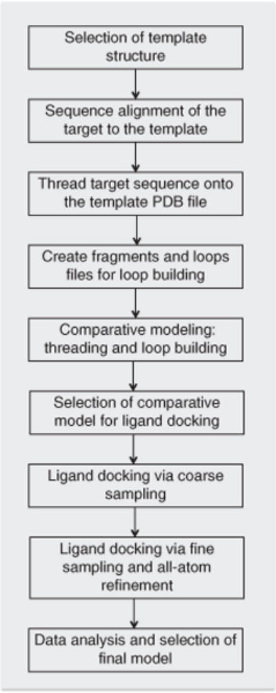
Outline of the Rosetta modeling protocol. This flowchart summarizes the complete protocol for docking small-molecule ligands into comparative models using Rosetta 3.4.

Comparative modeling with Rosetta

One of the most common applications of Rosetta is protein structure prediction via de novo folding and comparative modeling^8,9. De novo folding can be used to predict the protein’s tertiary structure when only the primary sequence of a protein is known. However, to date, Rosetta has been shown to successfully fold only small, soluble proteins (fewer than 150 amino acids), and it performs best if the proteins are mainly composed of secondary structural elements (α-helices and β-strands)¹⁰. Structures of helical membrane proteins between 51 and 145 residues were predicted to within 4 Å of the native structure¹¹, but only very small proteins (up to 80 residues) have been predicted to atomic-detail accuracy^12–14. Accurate prediction of larger and/or more complex proteins can be achieved with the addition of experimental data, such as NMR chemical shifts and distance data^15–17. Given these limitations, whenever an experimental structure of a related protein is available, comparative modeling is preferred to de novo folding.

Comparative modeling refers to the elucidation of the tertiary fold of a protein, which is guided by a known structure of another, often homologous, protein. The unknown structure is commonly called the ‘target’, whereas the protein of known structure, upon which the primary sequence of the target is threaded, is termed the ‘template’. The known template structure reduces the conformational search space by providing a protein backbone scaffold. Areas in which the template and target sequences diverge substantially are typically remodeled and refined using the loop-building application. The application is known as ‘loop building’ because it is most commonly applied to flexible loop regions between secondary structure elements. However, a ‘loop’ is defined here as any area where the backbone needs to be rebuilt de novo, which most often occurs in flexible regions but can also include secondary structural elements in cases of insertions/deletions or low sequence identity. Comparative models have played a major role in aiding experimental design and the interpretation of experimental results. They can be used to help predict structure-function relationships¹⁸, predict binding pockets for ligands during structure-based drug design¹⁹ and aid in the determination of target residues for site-directed mutagenesis^20,21.

In addition to Rosetta, other programs such as Modeller²² are often used to generate comparative models. Modeller is highly automated and, as with Rosetta, works best for cases in which the sequence identity between the target sequence and the template structure is greater than 30%. It works on the principle of satisfaction of spatial restraints derived from one or multiple templates. Comparative modeling in Rosetta⁵ is a multiple-step process that requires more input from the user; for example, user-specified loop definitions must be provided as input. These definitions can optionally be provided to Modeller, but they are not necessary in order for the program to run.

Ligand docking with RosettaLigand and comparison with other ligand-docking software

After a comparative model of the target protein has been constructed, computational ligand docking can be performed. Small-molecule ligand-docking applications attempt to predict the protein or small-molecule binding free energy, as well as critical binding interactions²³. These predictions can provide structural information of a ligand-binding site⁶, filter high-throughput screening libraries for likely hits^24,25 or guide de novo drug design^26,27. The protocol presented here details the process for small-molecule ligand docking and focuses on locating critical residues for binding a specific ligand.

RosettaLigand requires input structures of a receptor (protein) and a ligand (small molecule)^4,28,29. Because it does not perform binding pocket detection, the user must have prior knowledge of the location of the binding site. Other programs, such as SURFNET³⁰, LIGSITE³¹ and PocketDepth³², can be used to identify the ligand-binding site before using RosettaLigand for small-molecule docking. Ligand and receptor side-chain conformations are explored through Monte Carlo sampling of rotamers³³. Predicted protein-ligand interactions are deemed favorable and are accepted if they improve the Rosetta energy score (Box 1)⁴. Backbone flexibility of the protein is modeled using a gradient-based minimization of phi and psi torsion angles³⁴. Performing ligand docking with an ensemble of ligand conformations and protein backbones can be used to increase the conformational space sampled if the protein-ligand interaction does not fit the simple lock-and-key paradigm².

Box 1. The Rosetta energy function.

The energy, or scoring, function in Rosetta is derived empirically through analysis of observed geometries of a subset of proteins in the PDB. The measurements include, but are not limited to, radius of gyration, packing density, distance/angle between hydrogen bonds and distance between two polar atoms. The measurements are converted into an energy function through Bayesian statistics^35,84.

The scoring function in Rosetta can be separated into two main categories: centroid-based scoring and all-atom scoring. The former is used for de novo folding and initial rounds of loop building^1,35,85. The side chains are represented as ‘super-atoms,’ or ‘centroids,’ which limit the degrees of freedom to be sampled while preserving some of the chemical and physical properties of the side chain. Although this centroid-based scoring function is important for de novo folding, the folding protocol is not covered within the scope of this article.

The all-atom scoring function represents side chains in atomic detail. Similarly to the centroid-based scoring function, the all-atom scoring function comprises weighted individual terms that are summed to create a total energy for a protein. Most of the scoring terms are derived from knowledge-based potentials. The scoring function contains Newtonian physics–based terms, including a 6–12 Lennard- Jones potential and a solvation potential. The 6–12 Lennard-Jones potential is split into two terms, an attractive term ( fa_atr) and a repulsive term ( fa_rep), for all van der Waals interactions^86,87. The solvation potential ( fa_sol) models water implicitly and penalizes the burial of polar atoms88. Interatomic electrostatic interactions are captured through a pair potential ( fa_pair)⁸⁵, and an orientation-dependent hydrogen bond potential for long-range and short-range hydrogen bonding ( hbond_sc, hbond_lr_bb, hbond_sr_bb, and hbond_bb_sc, respectively)^89,90. In addition to the electrostatic terms, the Rosetta all-atom scoring function contains terms that dictate side chain conformations according to the Dunbrack rotamer library ( fa_dun)^33,84 preference for a specific amino acid given a pair of phi/psi angles ( p_aa_pp), and preference for the phi/psi angles in a Ramachandran plot ( rama)^9,90,91.

The accuracy of RosettaLigand was assessed by Davis and Baker⁴ by both retrospective and prospective benchmark studies. In 54 of 85 cases (64%), RosettaLigand’s top-scoring model was within 2.0 Å root mean square deviation (RMSD) from the experimentally determined structure. These results were achieved by including backbone and side-chain flexibility, as well as ligand flexibility through conformer selection and torsion angle adjustments.

Ligand-docking algorithms can be categorized on the basis of their scoring functions and search methodologies. RosettaLigand uses a knowledge-based scoring function derived from statistical analysis of the Protein Data Bank (PDB)³⁵. The conformational search of the binding site is accomplished using a Metropolis Monte Carlo algorithm^1–6,36. Other search strategies include geometric hashing (FlexX)³⁷, genetic algorithms (GOLD)³⁸ and systematic sampling (Glide)³⁹. Different scoring functions include physics-based force fields (Dock)⁴⁰, chemical descriptor models (FlexX³⁷) and knowledge-based potentials (RosettaLigand^4,28, DrugScore⁴¹).

A 2009 study compared the performance of the RosettaLigand docking method with nine other commonly used ligand-docking programs (Dock, Dockit, FlexX, Flo, Fred, Glide, GOLD, LigandFit, MOE and MVP)⁶. Ligand-docking algorithm performance was compared using a benchmark set of 136 ligands and eight target receptors provided by GlaxoSmithKline. This study demonstrated that the performance of RosettaLigand was comparable or better than the other ligand-docking algorithms considered. The study used crystallographic protein structures as inputs rather than comparative models. Kaufmann et al.⁴² demonstrated the predictive power of Rosetta ligand docking into Rosetta-built comparative models. In another study, RosettaLigand and AutoDock were used to dock 20 protein-ligand complexes⁴. In ten cases, RosettaLigand’s flexible backbone docking protocol found top-scoring models under 2.0 Å RMSD. In contrast, AutoDock identified only four such structures. However, the authors note that RosettaLigand consumed significantly more computational resources (40–80 CPU hours per input) than AutoDock (5–22 CPU hours per input)⁴.

Applying the comparative modeling and ligand-docking protocols to a single problem

To illustrate the entire comparative modeling and ligand-docking protocol on a single example, including a detailed analysis, we selected a target protein that has been co-crystallized with a small-molecule ligand and for which an experimental structure of a distantly related homolog is available to serve as a template. We also selected a relatively small protein and ligand to facilitate rapid reproduction of the protocols by the reader. Specifically, T4 lysozyme in complex with 1-methylpyrrole (PDB ID: 2ou0)⁴³ was chosen as the target and P22 lysozyme (Protein Data Bank (PDB) ID: 2anv)⁴⁴ as the template. Note that this selection was made with the above-mentioned didactic priorities in mind; it was not chosen in order to find an optimal system with which to benchmark the accuracy of Rosetta. Throughout the manuscript, we will refer to dedicated benchmark papers relevant to the individual steps to serve as references for expected Rosetta performance. In addition, Kaufmann and Meiler⁴² recently performed a benchmark of ligand docking into comparative models with Rosetta, to which the reader is encouraged to refer for further information concerning RosettaLigand’s performance for ligand docking into comparative models.

Experimental design

An overview of the entire protocol is summarized as a flowchart in Figure 1. The protocol involves construction of a comparative model and docking of the target ligand into the comparative model. It is important to consider the quality of the target protein/small-molecule complex at each decision-making step of the protocol: these considerations will be discussed at each crucial point.

In the procedure, we explicitly refer to the example of the construction of a comparative model of T4 lysozyme⁴³ based on the structure of P22 lysozyme⁴⁴ and of docking the ligand MR3 into the comparative model. For the purposes of illustration, the structure of T4 lysozyme is presumed to be unknown.

Template selection (Step 1)

In Rosetta, construction of a comparative model for a desired target protein can be divided into distinct steps. First, an experimentally determined structure (template) must be identified. The quality of a comparative model is heavily dependent on the experimentally determined structure that is chosen as a template for the final model. If a low-quality, low-resolution template structure is chosen, the resulting models will also be of low quality. The following discussion provides insight into the process of identifying a proper template for comparative modeling.

A template can be located with BLAST (http://www.ncbi.nlm.nih.gov/BLAST/), which searches the PDB for proteins with high sequence identity to the target sequence. In the BLAST server online, use ‘protein blast,’ and under ‘Database,’ choose to search the ‘Protein Data Bank (PDB),’ which contains all experimentally determined protein structures. A modified version of BLAST, PSI-BLAST, allows for the identification of distant members of a protein family using position-specific scoring matrices⁴⁵. Conversely, pattern hit–initiated BLAST (PHI-BLAST) treats two occurrences of the same pattern within the target sequence as two independent sequences and is useful for filtering out false positives when pattern occurrences are random⁴⁶. PSI-BLAST is the most commonly used method for identifying homologous proteins. Although there is no strict cutoff value for what is considered homologous, proteins with at least 30% sequence identity to the target protein and a BLAST e-value (the probability of seeing the alignment by chance) of <10⁻⁵ are suitable metrics for identifying homologous templates.

Although BLAST, PSI-BLAST and PHI-BLAST are commonly used for detecting homologs, other homology detection tools have been shown to be more accurate. For example, HHPred⁴⁷ and HMMER3 (refs. ^48,49) use profile hidden Markov Models (HMMs) to perform multiple sequence alignments. Similarly to simple sequence profiles, profile HMMs contain information concerning amino acid frequencies in each column of a multiple sequence alignment, but they also contain information about the frequency of insertions and deletions at each column. Therefore, methods that use profile HMMs potentially can be more sensitive than methods that use simple sequence alignments (for example, BLAST, PSI-BLAST).

Sometimes, homologous, experimentally determined structures cannot be identified for use as templates, in which case homology modeling would not be applicable. This problem can occur when sequence-comparison methods are not sensitive enough to detect remote homology. However, because structure is better-conserved evolutionarily than sequence, proteins with low sequence identity can have similar folds. In this case, 3D-fold recognition meta-servers, such as Phyre⁵⁰, can be used. Phyre performs a profile-profile alignment of the submitted sequence against its fold library to identify distantly related structures that are compatible with the target sequence. Once a suitable template has been identified, a sequence alignment should be performed between the target and template sequences (Steps 5–7).

Additional considerations should be taken into account when ligands are docked into comparative models. Kaufmann and Meiler⁴² demonstrated that ligand docking into templates of experimentally determined holo (ligand-bound) structures is more likely to be successful than docking into apo structures. The use of a holo structure as a template was more predictive of success than the overall template-to-target sequence identity or sequence similarity of residues in the binding site. Furthermore, ligand-bound template structures in which the ligands are similar to the target ligand should be prioritized; particular emphasis should be placed on ligands that share functional group placement similar to the target ligand. Finally, in order to obtain diversity of models that span the probable conformations of the target, multiple templates should be identified and carried through the comparative modeling process.

Sequence alignment and threading (Steps 5–9)

Once a template (or templates) has been identified, the primary sequence of the target protein is threaded onto the three-dimensional backbone of the template structure according to a sequence alignment of the two proteins. If the alignment of the two proteins results in a gap during alignment, the gap regions, which are usually indicated as dashes (‘-’) or spaces (‘ ’) in the alignment text file, are marked as loops in the newly generated threaded PDB file (Fig. 2). Further, the Cartesian coordinates for the gap region are set to 0.000, and the occupancy column is set to − 1.00 as an indicator to Rosetta that these atoms are to be generated de novo. For information on the PDB file format, see http://www.wwpdb.org/docs.html.Regions between secondary structure elements and areas where there is low confidence in the sequence alignment between the target and template proteins are then reconstructed with a loop-building protocol^51–53.

Figure 2.

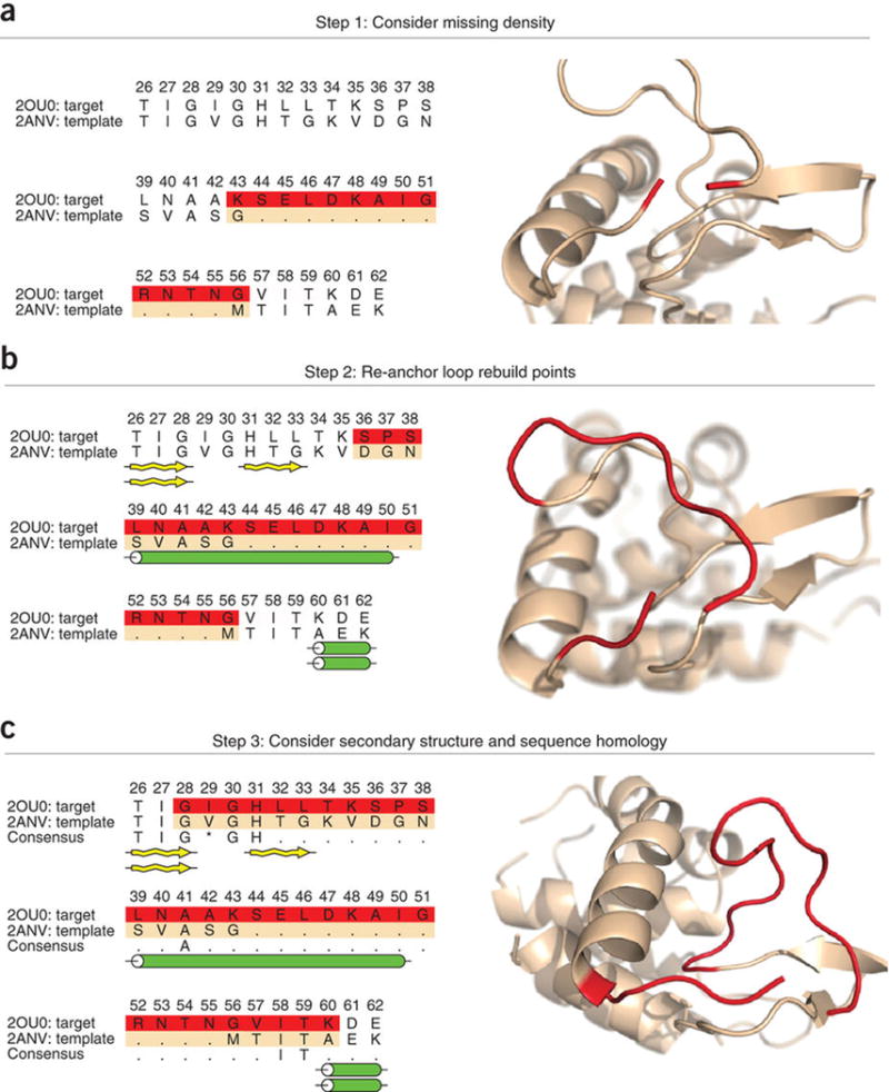
Criterion for selecting regions for de novo loop building. (a) The target sequence is threaded over the template backbone; the initial structure is shown in beige. There are 12 amino acids from the target sequence that do not have a corresponding amino acid from the template sequence (amino acids 44–55). The resulting alignment produces an insertion into the backbone of the template structure. To rebuild missing density, two anchor points, N- and C-terminal from the missing region, are chosen to remain fixed. The flanking amino acids of the areas of missing density (K43 and G56, highlighted in red) are chosen as the initial anchor points. Rosetta will perform de novo loop building in the area of missing density. (b) The two anchor points are repositioned, allowing enough space to rebuild the 12 amino acids. In addition to the 12-residue insertion, the region highlighted in red will be rebuilt with the de novo loop modeling protocol. (c) During de novo loop rebuilding, secondary structure is also taken into consideration. Target residues 39–50 and 31–33 are both predicted to have secondary structural elements, but the template sequence does not contain secondary structural elements at these positions. Therefore, the loop to be built is extended to include residues 39–50 and 31–33. The final anchor points G28 and K60 are chosen, allowing 31 amino acids to be rebuilt (shown in red).

Defining loop regions (Steps 10 and 11)

The loop definitions are chosen from the alignment between the target and template sequences. Regions having at least one of the following characteristics should be rebuilt as loops: (i) long coil regions with low sequence identity found in both template and target sequences; (ii) regions with discrepancies in secondary structural elements between the template and target secondary structure prediction (for example, a beta-sheet in the template was predicted to be a loop in the target); or (iii) missing density after threading the target sequence onto the template. This process is illustrated in Figure 2.

Rosetta includes two loop-building algorithms. Cyclic coordinate descent (CCD), inspired by inverse kinematic applications in robotics, adjusts residue dihedral angles to minimize the sum of the squared distances between three backbone atoms of the moving N-terminal anchor and the three backbone atoms of the fixed C-terminal anchor⁵¹. The advantages of CCD are its speed and its ability to close a loop over 99% of the time. Conversely, kinematic loop closure (KIC) analytically determines all mechanically accessible conformations for torsion angles of a peptide chain using polynomial resultants^52,53. Although KIC has been shown to recover loops from experimentally determined structures more accurately, it relies heavily on the location of the N- and C-terminal anchors and may not be an ideal choice for comparative modeling.

Rosetta loop building by CCD uses fragment libraries for generating loop coordinates for missing density in the threaded model. The fragment file comprises the target sequence divided into 3– and 9–amino acid overlapping sequence windows. There are 200 peptide fragments for each sequence window. After dividing the target primary sequence into 3– and 9–amino acid sequence windows, both Robetta and the fragment picker⁵⁴ application query a structural database of nonredundant proteins⁵⁵ for each peptide sequence and store the corresponding Cartesian coordinates and secondary structure information in fragment files. For more detailed background and information on this application, see Gront et al.⁵⁴ or go to http://www.rosettacommons.org/manuals/archive/rosetta3.4_user_guide/dc/d10/app_fragment_picker.html. Fragments can also be generated using NMR data using RosettaNMR¹⁵. For details on the procedure, please visit http://spin.niddk.nih.gov/bax/software/CSROSETTA/.

In this comparative modeling protocol, loop building takes place in two stages. In the first stage, a fast, low-resolution remodeling step with CCD consisting of broad sampling of backbone conformations is performed. In the second stage, the model is represented in all-atom detail and evaluated by Rosetta’s all-atom scoring function (Box 1). It has been suggested by Kaufmann and Meiler⁴² and others that ligands in the binding site of the template structure be carried into the comparative modeling process. Although this is not done here, it is anticipated that the use of such an approach would prearrange and maintain the pocket shape for small-molecule binding and result in higher-quality models of the protein-ligand complex.

All-atom refinement of the comparative model

The newly built model of the target protein undergoes refinement using the Rosetta all-atom scoring function (Box 1) to yield an all-atom protein model¹². Both comparative modeling and ligand docking in Rosetta involve an all-atom refinement of the protein. The protocol used for structural refinement, visually described in Figure 3, is often referred to as ‘relax.’ The goal of the relax protocol is to explore the local conformational space and to energetically minimize the protein. During this process, local interactions are improved by iterative side-chain repacking, in which new side chain conformations, or ‘rotamers,’ are selected from the Dunbrack library⁵⁶; and by gradient-based minimization of the entire model, in which the energy of the model is minimized as a function of the score. These small structural changes are evaluated according to the all-atom scoring function and are sampled in a Metropolis Monte Carlo³⁶ method. The relax protocol has been shown to markedly lower the overall energy of the Rosetta model and is essential to achieving atomic detail accuracy^1,13.

Figure 3.

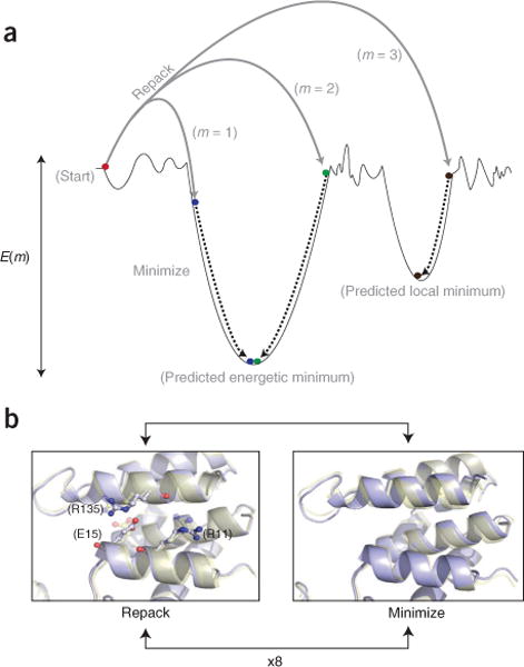
An overview of Rosetta energetic minimization and all-atom refinement via the relax protocol. (a) Simplified energy landscape of a protein structure. The relax protocol combines small backbone perturbations with side-chain repacking. The coupling of Monte Carlo sampling with the Metropolis selection criterion36 allows for sampling of diverse conformations on the energy landscape. The final step is a gradient-based minimization of all torsion angles to move the model into the closest local energy minimum. (b) Comparison of structural perturbations introduced by the repack and minimization steps. During repacking, the backbone of the input model is fixed, whereas side-chain conformations from the rotamer library33 are sampled. Comparison of the initial (transparent yellow) and final (light blue) models reveals conservation of the R135 rotamer but changes to the R11 and E15 rotamers. Minimization affects all angles and changes the backbone conformation.

Choosing a receptor model for ligand docking (Steps 14–16)

The quality of each comparative model is evaluated by a scoring function consisting of solvation, electrostatic interactions, van der Waals attraction or repulsion and hydrogen-bonding terms (Box 1)^13,57. As is the case with template selection, it is often difficult to identify a single model that will ultimately provide the correct conformation of the docked ligand. Therefore, multiple structures resulting from comparative modeling should be used as input for ligand docking. These inputs are selected by pooling all models, regardless of template heritage, and then selecting a small percentage that fall below a certain energy cutoff. The top-scoring models, which are those within a certain percentage or score of the best model, are then clustered (Supplementary Discussion) and carried forward into ligand docking. Clustering ensures that a maximally diverse set of models is used.

Ligand docking into comparative models (Steps 17–22)

Next, the small molecule to be docked is placed into the binding site of each Rosetta model. For the best results, the target ligand is initially placed in a similar position to small molecules found in the original template structures. Ideally, biochemical information, such as results obtained from mutagenesis studies, can be used to inform the docking by restricting the conformational sampling space. If water molecules and cofactors are known to bind to the receptor, they can be added to the comparative models and docked simultaneously²⁹. For simplicity, this feature is not demonstrated in our protocol.

The Rosetta ligand-docking algorithm first translates the ligand within a user-specified radius. These translations are repeated until the ligand’s geometric center sits in a position that is not occupied by atoms in the receptor. These translations are followed by up to 1,000 cycles of random rotation. A conformation resulting from rotation, in which the attractive and repulsive scores fall below a threshold value, is chosen for further refinement. Alternatively, if the position and orientation of the ligand is known, particularly if the target protein-ligand complex is highly homologous to an experimentally determined structure, then the translation/rotation movements described above may not be necessary and can be omitted.

In the high-resolution refinement step, six cycles of side-chain rotamer sampling are coupled with small (0.10 Å, 0.05 radians) ligand movements. Each cycle includes minimization of ligand torsion angles with harmonic constraints, where 0.05 radians of movement is equal to 1 s.d. of the harmonic function. Amino acid side chains are repacked using a backbone-dependent rotamer library³³. During refinement, the weight of Rosetta’s repulsive score term is decreased, thus preventing model rejection due to minor inter-atomic clashes. In a final energy minimization step, side chain rotamer sampling is coupled with minimization of backbone torsion angles. This is conducted with harmonic constraints on the α-carbon atoms (0.2 Å s.d.).

Several metrics can be used to evaluate the results obtained from ligand docking. The most common evaluation method is analysis of the Rosetta energy, which is measured in Rosetta energy units (Box 1). Generally, models having lower, more negative Rosetta energies are considered to be more native-like⁵⁸. Kaufmann and Meiler⁴² observed that the native conformation of the complex is almost always sampled. However, when docking ligands into comparative models, the energy landscape is often rough, resulting in poor scores of the native complex. To account for this, the models can be clustered in order to group the models by structural similarity (Supplementary Discussion). An appropriate clustering radius should be chosen on the basis of ligand size. Representative models are then chosen from each cluster according to score. Clustering and score analysis reduce the data from thousands of models to a manageable number necessary to carry out an accurate, meaningful analysis. This clustering process often results in up to 20 conformations of similar validity. Experimental data can be used to confirm a particular binding mode, or experiments can be designed and executed to differentiate the possible conformations. Furthermore, these restraints can be used to guide the modeling process (Supplementary Discussion).

Use of experimental restraints during Rosetta modeling and analysis

Incorporation of experimental data into structure prediction and analysis has been shown to improve the quality of the final model or ensemble of models^15,59–61. Numerous types of experimental data have been incorporated into such protocols, including electron density from X-ray crystallography⁶² and electron microscopy, NMR distance and orientation data^60,63, EPR distance data^59,61, cross-linking restraints⁶⁴, small-angle X-ray scattering data⁶⁵ and deuterium-exchange mass spectrometry data⁶⁶. Although these types of data are more often applied to de novo protein structure elucidation, they can also be of some use in loop building⁶⁷, reorientation of domains during comparative modeling or identification of residues involved in ligand binding. Experimental data can also be used to filter out models during postprocessing. Post hoc analysis allows for incorporation of data not easily represented as a restraint during model building. By performing rank-order predictions of binding energies, enzyme activities or mutational effects, and comparing these with known biochemical data, the correct model can be differentiated from those that do not agree with experimental observations^18,68,69. If restraints are not available, validation of the model should be obtained by experiments inspired by the computational results.

Caveats and challenges

As with all computational techniques, there are caveats associated with using Rosetta for comparative modeling and ligand docking. Although comparative modeling can be used to model large proteins more reliably than de novo folding methods, it is limited by the availability of high-quality structural templates in the PDB. Finite computational resources can also limit the size of conformational spaces that can be searched⁷⁰. The comparative modeling and ligand-docking processes discussed in this protocol allow for protein backbone movement. However, these models represent only static structures of local energy minima. For consideration of dynamics, conformational changes and large-scale changes due to induced-fit or conformational flexibility during ligand docking, molecular dynamics simulations have been shown to be useful⁷⁰.

Despite these limitations, Rosetta has been used to produce protein models that have proven invaluable where no experimentally determined protein structure exists^19,68,71. The presented protocol, which refers to T4 lysozyme throughout as a simple example, provides a generalized workflow for comparative modeling and ligand docking in the Rosetta framework, and also demonstrates its ability to model accurate protein structures.

Availability

Rosetta is available through software licenses processed by the RosettaCommons (http://www.rosettacommons.org). Licenses for academia and nonprofit institutions are free of charge. The Rosetta software suite can be installed on a Linux or OSX operating system (Supplementary Discussion). This setup allows other researchers to adopt the described protocol for their biological system of interest.

MATERIALS

EQUIPMENT

Starting data

• Primary sequence of target protein

• High-resolution protein structure of a homolog to the target sequence

• Desired small molecule for ligand docking

Hardware and software

• Linux- or MacOS-based workstation with internet access

• Plain text editor, such as vi, vim or emacs

• Academic or commercial copy of Rosetta obtained from http://www.rosettacommons.org/software/

• Access to the Robetta server (http://robetta.bakerlab.org). Note that commercial users cannot use this server; instead, they must use this file for Step 10: http://www.bioshell.pl/rosetta-related/vall.apr24.2008.extended.gz

• Python, with BioPython and numpy installed (Supplementary Discussion)

• Optional: Linux- or BlueGene/L-based cluster

PROCEDURE

Selection of a template ● TIMING 15 min

• 1|Select a template for comparative modeling of the target protein. Template selection is the conceptual first step of any comparative modeling procedure and is discussed in the Experimental design section. It is often beneficial to explore multiple templates as well. In this procedure, the target protein to be modeled is T4 lysozyme⁴³, and the template being applied is the structure of P22 lysozyme⁴⁴.

  ? TROUBLESHOOTING

Preparing the PDB file of the template structure ● TIMING 5 min

• 2|Download the template PDB file from the PDB at http://www.rcsb.org. The template PDB can be found by searching for the four-letter PDB ID, ‘2anv.’
• 3|
  Format, or ‘clean,’ the protein to avoid errors when Rosetta reads in the PDB file. Cleaning the PDB file simplifies it for Rosetta by removing non-ATOM records, renumbering residues and atoms from 1 and correcting chain ID inconsistencies. The script clean_pdb.py, located in the rosetta_tools/protein_tools/scripts/ directory, will be used to format the template PDB file (see Supplementary Discussion for instructions on installing the necessary python modules). The script follows the following format:

  python rosetta_tools/protein_tools/scripts/clean_pdb.py <raw_pdb_file> <chain>
  

  Execute the script by typing the following:

  python rosetta_tools/protein_tools/scripts/clean_pdb.py 2anv.pdb A
  The script will output two files: 2anv_A.pdb and 2anv_A.fasta
  

  ? TROUBLESHOOTING

• 4|Relocate the created FASTA and PDB files from the script to an input_files directory, which will be used in subsequent steps. The output to the screen is used for error checking and can be disregarded if no errors occurred.

Sequence alignment ● TIMING 15 min

• 5|
  Generate a FASTA file for the target sequence. A FASTA file is a text file that contains a header line, which consists of the name of the protein, followed by the amino acid sequence of the protein on a separate line; this is indicated below:

  > 2ou0:X|PDBID|CHAIN|SEQUENCE
  MNIFEMLRIDEGLRLKIYKDTEGYYTIGIGHLLTKSPSLNAAKSELDKAIGRNTNGVITKDEAEKLFNQDVDAAVRGILRNAKL KPVYDSLDAVRRAAAINMVFQMGETGVAGFTNSLRMLQQKRWDEAAVNLAKSRWYNQTPNRAKRVITTFRTGTWDAYK
  

  The target FASTA file that is used comes from the T4 lysozyme sequence. The FASTA file can be downloaded from the PDB by searching for ‘2ou0’ in the search bar at the top of the webpage. Download the FASTA file for the target by clicking on ‘Download’ to the right of the PDB ID and selecting ‘FASTA.’ Save the file as 2ou0_.fasta. The header line for the 2ou0_.fasta file must be edited. Replace the text

  > 2ou0:X|PDBID|CHAIN|SEQUENCE
  with
  > 2ou0_
  

  The FASTA file 2anv_A.fasta that was created from Step 3 can be used for the template sequence.

• 6|Run ClustalW on the web server (http://www.ebi.ac.uk/Tools/msa/clustalw2/) by pasting the contents of the two FASTA files into the box labeled ‘STEP 1—Enter your input sequences.’ The order of the FASTA files is irrelevant. Both sequences should be in FASTA format, i.e., they must start with a header line such as > target_sequence or> template_sequence, followed by the sequence on a new line (Step 5). On ‘STEP 2,’ select ‘slow’ for the ‘alignment type.’ This will provide the most accurate alignment for the two sequences. Do not change anything in the ‘STEP 3’ box, and hit the ‘Submit’ button on ‘STEP 4.’ After a short wait, a new page will be loaded in which the alignment can be downloaded and saved. Click on the button labeled ‘Download Alignment File.’ Several sequence alignment tools are publicly available; here we use the web server, ClustalW⁷² for its simplicity and accessibility. If a different alignment tool is used, the output from the alignment must be in one of the following formats: Clustal, EMBOSS, FASTA, FASTA-M10, IG, Nexus, PHYLIP or Stockholm.

  ? TROUBLESHOOTING

• 7|Save the alignment file as alignment.aln in the current working directory. The default suffix provided by ClustalW is.clustalw.

Threading ● TIMING 15 min

• 8|
  Thread the target sequence over the template structure using the included script. The script has the following format:

  python rosetta_tools/protein_tools/scripts/thread_pdb_from_alignment.py–template = <name of template in alignment file>–target = <name of target in alignment file>–chain = <chain in pdb>–align_format = clustal <alignment file> <template. pdb> <output.pdb>
  

  The– template and – target must match the names given in the file of the FASTA file. Check the target and template names by opening the alignment file that was created in Step 6. If the naming has been consistent according to the previous steps, the command used to thread the template PDB should be:

  python rosetta_tools/protein_tools/scripts/thread_pdb_from_alignment.py–template = 2anv_A–target = 2ou0_–chain = A –-align_format = clustal alignment.aln 2anv_A.pdb 2ou0_threaded.pdb
  

  ! CAUTION The result of Step 8 ( 2ou0_threaded.pdb) is a PDB file that Rosetta will use as input. Examine this file with a text editor and also with a 3D protein structure viewer, such as PyMOL (http://www.PyMOL.org/) or Chimera⁷³ (http://www.cgl.ucsf.edu/chimera/), in order to ensure that it contains the intended target sequence, that the conserved regions (especially helices and strands) between target and template are preserved and that insertions (residues present in target but not template) have zero (0.000) Cartesian coordinate values and − 1.00 occupancy values.

  ? TROUBLESHOOTING

• 9| Verify that the 2ou0_threaded.pdb sequence matches the target primary sequence by generating a FASTA file from the PDB using the included script. This script has the following syntax:

  python rosetta_tools/protein_tools/scripts/get_fasta_from_pdb.py <template_pdb> <chain> <output fasta file>
  

  If the naming has been consistent, the command issued will be as follows:

  python rosetta_tools/protein_tools/scripts/get_fasta_from_pdb.py 2ou0_threaded.pdb A 2ou0_threaded.fasta
  

  Submit the two sequences 2ou0_.fasta and 2ou0_threaded.fasta to the ClustalW server (http://www.ebi.ac.uk/Tools/msa/clustalw2) to verify that the sequences match.

Preparation of fragment files of the target sequence ● TIMING 15–60 min

• 10| Generate fragment files of the target sequence. There are two commonly used methods to generate fragments for comparative modeling. Users affiliated with a nonprofit institution can use the Robetta server (http://www.robetta.org/), which is described in option A. Conversely, for-profit organizations should follow option B to use the fragment picker application that comes with the Rosetta source code.

  1. Creating fragment files with Robetta

     1. Register for a username and password at the Robetta web server (http://robetta.bakerlab.org/fragmentsubmit.jsp).

     2. Input the sequence name 2ou0_, and load the target FASTA file, 2ou0_.fasta, from Step 5.

     3. Submit the FASTA file. The webpage will reload and state ‘Successfully added your request to the queue.’ The status of the fragment file generation can be checked at http://robetta.bakerlab.org/fragmentqueue.jsp.

     4. Click the link to get a list of files generated by Robetta after the status has changed to ‘Complete.’ If you are following the example of 2ou0 for the target sequence, the fragment files should be called aa2ou0_003_05.200_v1_3 for fragments of length 3 and aa2ou0_009_05.200_v1_3 for fragments of length 9. Save all the files to the working directory by right-clicking and selecting ‘Save as.’

  2. Creating fragment files with the fragment picker

     ? TROUBLESHOOTING

     1. Generate a secondary structure prediction file from a server, such as PSI-PRED⁷⁴ (http://bioinf.cs.ucl.ac.uk/psipred/) or JUFO9D (ref. 75) (http://www.meilerlab.org/index.php/servers/show). In either case, the primary sequence of the target protein must be in FASTA format.

        ! CAUTION The fragment picker expects PSI-PRED vertical format for all secondary structure prediction files. If PSI-PRED is used to generate secondary structure predictions, make sure to select the ‘machine learning scores’ option when downloading the results. If JUFO9D is used, download the three-state secondary structure prediction file ( .jufo9d_ss), and then make the following PSI-PRED header the first line of the JUFO9D prediction file, followed by a blank line:

        # PSIPRED VFORMAT (PSIPRED V3.0)
        

     2. Generate a sequence profile (checkpoint file). The sequence profile is created by PSI-BLAST. This file can be generated by running the Rosetta make_fragments.pl script with the following options:

        rosetta_tools/fragment_tools/make_fragments.pl-id 2ou0_-nopsipred – psipredfile <psi_pred_file>-nosam –nojufo 2ou0_.fasta
        

        The psi_pred_file was generated from the secondary structure prediction (Step 10B(i) above). The checkpoint file will be named 2ou0_.checkpoint.

     3. Create a fragment-picking weights file called QuotaProtocol.wts

        # score name priority weight min_allowed extras
        SecondarySimilarity	350	0.5	-	psipred
        SecondarySimilarity	250	0.5	-	JUFO
        RamaScore	150	1.0	-	psipred
        RamaScore	150	1.0	-	JUFO
        ProfileScoreL1	200	1.0	-
        PhiPsiSquareWell	100	0.0	-
        FragmentCrmsd	30	0.0	-

     4. Create a quota definition file called QuotaProtocol.def

        #pool_id	pool_name	fraction
        1	psipred	0.6
        2	JUFO	0.2

     5. Create a fragment-picking options file called fragment.options in a text editor. The file should have the following format:

        -database <path to Rosetta Database>
        -in:file:vall <path to Vall Database> # available from Rosetta checkout
        -in:file:fasta 2ou0_.fasta
        -in:file:s 2ou0_threaded.pdb
        -in:file:checkpoint 2ou0_.checkpoint
        -frags:ss_pred 2ou0_.psipred.ss2 psipred 2ou0_.jufo9d_ss JUFO
        -frags:scoring:config QuotaProtocol.wts
        -frags:picking:quota_config_file QuotaProtocol.def
        -frags:frag_sizes 9 3
        -frags:n_candidates 1000
        -frags:n_frags 200
        -out:file:frag_prefix 2ou0_quota
        -frags:describe_fragments 2ou0_quota.sc
        

     6. Run the following command line:

        rosetta_source/bin/fragment_picker.default.OperatingSystemrelease @fragment.options
        

        With the fragment picker, the fragment files will be output as 2ou0_quota.200.3mers and 2ou0_quota.200.9mers.

Creating a Rosetta loops file ● TIMING 5 min

• 11|
  Create a file that defines loop regions to be rebuilt. One line per loop should be written to a file with the extension .loops (e.g., 2ou0_.loops). The Rosetta loop building protocol will rebuild regions between residues specified in the loops file. The information in the loops file is explained further in Table 1.

  LOOP	28	60	0	0	0
  LOOP	81	93	0	0	0
  LOOP	112	126	0	0	0
  LOOP	135	151	0	0	0

  ? TROUBLESHOOTING

TABLE 1.

Explanation of information contained in the loops file (Step 11).

Column 1	LOOP	The loops file identity tag
Column 2	<integer>a	Loop start residue number. Note: the starting structure must have real coordinates for all residues outside the loop definition, plus the first and last residue of each loop region
Column 3	<integer>	Loop end residue number
Column 4	<integer>	Cut point residue number, must be greater than the first residue of the loop and less than the end residue of the loop. Default (0)—let loop rebuild protocol choose cut point
Column 5	<float>	Skip rate. Default (0)—never skip
Column 6	<boolean>	Extend loop. Default (0)—false

^aThe <> indicates areas where the user is to specify the integer, float or boolean (0 for false or 1 for true).

Preparation of comparative modeling options file ● TIMING 5 min

• 12|
  Create an options file with the name modeling.options and add the lines below. Comments within the options file are ignored when the ‘#’ tag precedes them. For more information on Rosetta options files, see Box 2.

  -loops:input_pdb 2ou0_threaded.pdb #input file
  -loops:fa_input #input will be in all-atom mode
  -loops:loop_file 2ou0_.loops #loop definitions
  -loops:frag_sizes 9 3 1 #sizes of fragments
  -loops:frag_files aa2ou0_09_05.200_v1_3 aa2ou0_03_05.200_v1_3 none #location of the fragment files. Fragments files will have the extension.quota.200.3mers and.quota.200.9mers if created with the fragment picker
  -loops:remodel quick_ccd #the centroid phase of loop modeling using CCD
  -loops:refine refine_kic #the all-atom phase of loop modeling
  -loops:extended true #forces an extended conformation on loops, independent of loop input file. For rebuilding loops entirely. Phi-psi angles will be set to 180 degrees in the first step. 
  -loops:idealize_after_loop_close #give idealized phi and psi angles after it has been closed
  -loops:relax fastrelax #does a minimization of the entire structure in the torsion space
  -loops:fast #decreases the monte carlo inner and outer cycles of loop rebuilding, greatly decreasing computation time
  -ex1 #rotamer libraries used in the repack steps
  -ex2
  

  ? TROUBLESHOOTING

Box 2. The Rosetta options file.

The Rosetta options file allows users to pass specific protocol-related parameters to a specific Rosetta application. The options file is often called the ‘flags’ file. Options can be accessed by the command line, placed within a file or some combination of both. Shown below is an example of a Rosetta options file. Note that lines beginning with # are comments and are ignored when running Rosetta. Words in <> indicate where, in a specific case, the actual path to the necessary file would go (with no <>).

-database <database> # database location
-in
 -file
   -s <protein.pdb> #name of PDB file
  -out
 -prefix <desired_prefix> #desired output prefix of results files
-packing
  -ex1 #use extra rotamer conformations for chi 1
  -ex2 #use extra rotamer conformations for chi 2
  -repack_only #changes Rosetta’s default redesign behavior

! CAUTION The space formatting of the options file is crucial. In the example above, each new ‘namespace’ (e.g., database, in, out, packing) starts a new line, and the ‘subspaces’ (e.g., file) are indented by a space or a tab. However, tabs and spaces cannot be mixed within the same file.

An alternate format for the options file is as follows:

-database <database>
-in:file:s <protein.pdb>
-out:prefix <desired_prefix>
-packing:ex1
-packing:ex2
-packing:repack_only

In the above example, subspaces are designated by a colon (e.g., ex1 is a subspace option of the namespace packing; therefore, -packing:ex1.)

! CAUTION If you are using RosettaScripts92, which requires the input of an XML file (Box 3), the options specified in this XML file override the options specified in the options file or those passed over the command line; therefore, it is important to avoid conflicting or contradicting options.

Running the comparative modeling job ● TIMING 5,000 CPU hours for 10,000 models

• 13|
  Generate comparative models of the target protein using Rosetta. At this point, only the Rosetta loop-building application is needed. A benchmarking study of loop building in Rosetta with CCD can be found in Wang et al.⁷⁶. The following command can be used to run loop modeling in Rosetta. In the command line, OperatingSystem should be replaced with the operating system of the machine on which the job is running. For example, if the job is running on a Linux machine, the name of the executable will be loopmodel.default.linuxgccrelease. This command is executed on a single processor and produces 10,000 models.

  rosetta_source/bin/loopmodel.default.OperatingSystemrelease @modeling.options-database rosetta_database-nstruct 10000
  

  ! CAUTION It is advised to split the generation of models across multiple computers or multiple CPUs on one computer. For example, one could start four different jobs on four different processors. Each job would have its own command line, varying only the – out:prefix <prefix> or –out:suffix <suffix> options to give each job its own unique name. Each job would only generate 2,500 unique structures, summing to 10,000 when all four jobs are complete.

  ? TROUBLESHOOTING

Analyzing and selecting models for ligand docking ● TIMING 60 min

• 14|Choose the ten lowest-energy comparative models for the ligand-docking steps below. Rename the files to model_01.pdb, model_02.pdb … model_10.pdb. The process of choosing models to be used in ligand docking can vary depending on the user’s specific biological problem (see Experimental design). As seen in Figure 4, the lowest-energy models are reasonably close to the native structure and, as such, are a good starting point for ligand docking. These models are commonly chosen based on overall energy according to Rosetta’s scoring function (Box 1), because they are usually low-energy models with fully closed loops and minimal inter-atomic clashes. Other modes of filtering, such as model satisfaction of experimental restraints (Supplementary Discussion) or clustering (Supplementary Discussion), can also be used. Furthermore, increased sampling of regions that do not converge on one or several conformations can improve the final model during de novo protein folding^14,58,77.

  ? TROUBLESHOOTING

• 15|Use a 3D protein structure viewer to check the receptor models visually. Models to be used for ligand docking should not have chain breaks, missing atoms/residues, overlapping atoms or unrealistic geometry.
• 16|Align the ten comparative models using any 3D protein structure viewer and save the resulting coordinates to new, individual PDB files before moving on to the ligand-docking part of the protocol. A benchmarking study of comparative modeling in Rosetta can be found in Misura et al.⁵.

Figure 4.

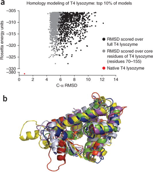
Building loops in comparative models of T4 lysozyme. Loops were rebuilt in comparative models of T4-lysozyme using P22 lysozyme as a template, as detailed in Steps 1–13 of the protocol. (a) The RMSD of C^α atoms between 10,000 models and the native protein (PDB ID: 2ou0) was computed over the full protein (black) and the core residues of T4 lysozyme (gray). The top 10% of models by Rosetta energy are shown here. Generally, a low Rosetta energy correlates with a low RMSD. For comparison, the Rosetta energy for the energy-minimized native crystal structure is shown in red. (b) Five of the lowest-energy models are seen in comparison with the native structure (shown in gray).

Preparing the ligand file for input to Rosetta ● TIMING 15 min

• 17|Obtain a representation of the ligand to be docked of the type mol, mol2 or sdf. If a protein structure is determined in the presence of a ligand of interest, an sdf file can be downloaded from the PDB; however, hydrogen atoms are usually not present and must be added. To generate a mol file from a pdb (PDB) file, many different software packages can be used, including MOE (http://www.chemcomp.com/index.htm), PyMOL and ChemDraw (http://www.cambridgesoft.com/software/ChemDraw/). Generation of the mol file is not covered within this Protocol.
• 18|
  Run the following command to convert a mol file into a params file. Rosetta reads in ligand information files from a params file. The params file contains information about the atoms, bonds, charge and coordinates of a ligand. The params file is generated from a molecule file, which can be of the type mol, mol2 or sdf.

  python rosetta_source/src/python/apps/public/molfile_to_params.py <mol file>
  

  In this specific example, 1-methyl-1H-pyrrole (MR3) is in complex with 2ou0 and is the ligand that will be docked into the comparative model of T4 lysozyme (2ou0). The command line used to create a params file for MR3 is as follows:

  python rosetta_source/src/python/apps/public/molfile_to_params.py-n MR3 MR3.mol
  

  Where -n MR3 is the three-letter name for the ligand. The resulting output will be MR3.params and MR3_0001.pdb.

  ? TROUBLESHOOTING

• 19|Add the ligand structure to the files containing the protein models. By using a text editor, copy the lines from MR3_0001.pdb and paste them to the bottom of each of the ten model PDB files from Steps 14–16. The resulting files will be used as docking input.

Preparation of the ligand-docking XML file ● TIMING 5 min

• 20|
  Create a ligand-docking XML file. The scoring functions, filters and movers (specific Rosetta functionalities for the protocol) are specified in the XML file (Box 3). Given below is an example of an XML file, named ligand_dock.xml, that will be used to dock the ligand MR3 into the T4 lysozyme comparative models chosen in Steps 14–16. Comments on specific steps are shown outside of the <>. It should be noted that comments are handled differently between the XML file and the options file. We recommend beginning with the provided XML file and altering key variables to suit the specific needs of the study.

  <ROSETTASCRIPTS>
   <SCOREFXNS>
    <ligand_soft_rep weights = ligand_soft_rep>
     <Reweight scoretype = hack_elec weight = 0.42/>
     <Reweight scoretype = hbond_bb_sc weight = 1.3/>
     <Reweight scoretype = hbond_sc weight = 1.3/>
     <Reweight scoretype = rama weight = 0.2/>
    </ligand_soft_rep>
    <hard_rep weights = ligand>
     <Reweight scoretype = fa_intra_rep weight = 0.004/>
     <Reweight scoretype = hack_elec weight = 0.42/>
     <Reweight scoretype = hbond_bb_sc weight = 1.3/>
     <Reweight scoretype = hbond_sc weight = 1.3/>
     <Reweight scoretype = rama weight = 0.2/>
    </hard_rep>
   </SCOREFXNS>
   <LIGAND_AREAS>
    <docking_sidechain_X chain = X cutoff = 6.0 add_nbr_radius = true all_atom_mode = true minimize_ligand = 10/>
    <final_sidechain_X chain = X cutoff = 6.0 add_nbr_radius = true all_atom_mode = true/>
    <final_backbone_X chain = X cutoff = 7.0 add_nbr_radius = false all_atom_mode = true Calpha_restraints = 0.3/>
   </LIGAND_AREAS>
    <INTERFACE_BUILDERS>
     <side_chain_for_docking ligand_areas = docking_sidechain_X/>
     <side_chain_for_final ligand_areas = final_sidechain_X/>
    <backbone ligand_areas = final_backbone_X extension_window = 3/>
    </INTERFACE_BUILDERS>
   <MOVEMAP_BUILDERS>
    <docking sc_interface = side_chain_for_docking minimize_water = true/>
    <final sc_interface = side_chain_for_final bb_interface = backbone minimize_water = true/>
   </MOVEMAP_BUILDERS>
   <MOVERS>
  single movers
   <StartFrom name = start_from_X chain = X>
    <Coordinates × =−18.8922 y = 24.5837 z = −5.7085/>
   </StartFrom>
   <CompoundTranslate name = compound_translate randomize_order = false allow_overlap = false>
    <Translate chain = X distribution = uniform angstroms = 2.0 cycles = 50/>
   </CompoundTranslate>
   <Rotate name = rotate_X chain = X distribution = uniform degrees = 360 cycles = 500/>
   <SlideTogether name = slide_together chain = X/>
   <HighResDocker name = high_res_docker cycles = 6 repack_every_Nth = 3 scorefxn = ligand_soft_rep movemap_builder = docking/>
   <FinalMinimizer name = final scorefxn = hard_rep movemap_builder = final/>
   <InterfaceScoreCalculator name = add_scores chains = X scorefxn = hard_rep/>
  compound movers
   <ParsedProtocol name = low_res_dock>
    <Add mover_name = start_from_X/>
    <Add mover_name = compound_translate/>
    <Add mover_name = rotate_X/>
    <Add mover_name = slide_together/>
   </ParsedProtocol>
   <ParsedProtocol name = high_res_dock>
    <Add mover_name = high_res_docker/>
    <Add mover_name = final/>
   </ParsedProtocol>
   </MOVERS>
   <PROTOCOLS>
    <Add mover_name = low_res_dock/>
    <Add mover_name = high_res_dock/>
    <Add mover_name = add_scores/>
   </PROTOCOLS>
  </ROSETTASCRIPTS>
  

  LIGAND_AREAS are used to describe the degree of protein and ligand flexibility in proximity to the protein-ligand interface. A cutoff value of 6.0 Å means that any residue within 6.0 Å of the ligand will be considered part of the interface. These values can be increased or decreased to enlarge or reduce the number of protein residues selected for rotamer sampling or backbone flexibility. The minimize_ligand value can be increased or decreased to alter the degree of ligand flexibility. This value represents the size of one standard deviation of movement in degrees. The Calpha_restraints value represents 1 s.d. of α-carbon movement in angstroms (Å) and can be enlarged or reduced to alter the degree of backbone flexibility.

  The coordinates given to the StartFrom mover should be adjusted to represent starting points for ligand docking. Typically, experimental data are used to determine the initial site of ligand docking. For this example, extensive experimental data have identified a small, buried hydrophobic binding site centered at A99 (ref. 43). An average was taken over the Cartesian coordinates for the β-carbon atom of A99 from each of the ten models for the StartFrom mover in the script above.

  The Translate mover’s ‘ angstroms’ field should be adjusted to represent the size of the binding pocket that needs to be sampled. Because the ligand in this case is small, the ligand is allowed to translate within a 2.0-Å radius of the starting coordinates. As familiarity with the provided ligand-docking XML protocol is accrued, experiment with developing a custom protocol. Typically, if no experimental data on ligand binding is present, a 5.0-Å radius is used.

  ? TROUBLESHOOTING

Box 3. RosettaScripts XML file.

RosettaScripts is an XML scriptable interface to the Rosetta software with a variety of movers, scoring functions and filters that can be tailored to a custom protocol⁹². Movers are defined as steps in the protocol that can change the conformation of the system being modeled, or ‘pose.’ Examples of movers include docking, loop building and gradient-based minimization. Filters are used to decide whether a given pose should proceed to the next step of the protocol. (Scoring functions are discussed in Box 1.) RosettaScripts protocols are versatile and can consist of a ‘mix-and-match’ set of user-defined movers, filters and scoring functions. This allows for complete customization of a protocol without manually editing the Rosetta source code. The XML file is divided into five sections: scoring functions, filters, movers, constraints and protocols. The format is shown below with generic names given for each section. For UserScoreFunctionName, UserFilterName and UserMoverName, the user can choose a name for the scoring function or filter. For RosettaMoverName, the name of the mover, as well as the options that accompany it, must be specified. Further information can be found at http://www.rosettacommons.org/manuals/archive/rosetta3.4_user_guide/Movers_(RosettaScripts).html.

<ROSETTASCRIPTS>
 <SCOREFXNS>
  <UserScoreFunctionName weights = “standard”/>
 </SCOREFXNS>
 <FILTERS>
  <UserFilterName name = “filter”/>
 </FILTERS>
 <MOVERS>
  <RosettaMoverName name = “UserMoverName” score = Scorefxnname/>
  <RosettaMoverName name = “userMoverName1” score = Scorefxnname/>
  <RosettaMoverName name = “UserMoverName2” score = Scorefxnname/>
 </MOVERS>
 <APPLY_TO_POSE>
 </APPLY_TO_POSE>
 <PROTOCOLS>
  <Add mover_name = “UserMoverName”/>
  <Add mover_name = “UserMoverName1” filter_name = “UserFilterName”/>
  <Add mover_name = “UserMoverName2”/>
 </PROTOCOLS>
</ROSETTASCRIPTS>

This generic XML file combines three separate movers that are scored by a user-defined scoring function ( UserScoreFunctionName), where UserMoverName1 will be repeated until UserFilterName is satisfied. The input protein, the pose, steps through each mover iteratively until the final step is completed. The output is the final score of the pose and is given as a score file and/or the 3D coordinates of the final pose.

Preparation of the ligand-docking options file ● TIMING 5 min

• 21|
  Create an options file called ligand_dock.options. In addition to the input PDB ( -in:file:s) and the database location ( -database), ligand params files (generated in Step 18) must be provided ( -in:file:extra_res_fa). The name of the XML file must be provided ( -parser:protocol). PDB files are output by default. Given below is the options file used for ligand docking in this example:

  -in:file:s model_01.pdb #this option will need to be changed for each of the ten models used in the docking protocol, for example, model_10.pdb
  -in:file:extra_res_fa MR3.params
  -packing:ex1
  -packing:ex2
  -parser:protocol ligand_dock.xml
  

  Accurate predictions of interfaces often rely on fine-grained placement of side chain atoms. Thus, it is recommended that the number of side chain rotamers be increased to include the standard rotamer plus or minus 1 s.d. This is accomplished as shown under the packing option group ( -packing:ex1, -packing:ex2). See the Rosetta documentation for additional rotamer selection options.

Running the ligand-docking job ● TIMING 16 CPU hours for 10,000 models

• 22|
  Run the ligand-docking job by specifying the executable and the options file on the command line:

  rosetta_source/bin/rosetta_scripts.default.OperatingSystemrelease @ligand_dock.options-database rosetta_database-nstruct 1000
  

  The number of models ( -nstruct) necessary to produce high-quality predictions will depend on the size of the binding pocket and the flexibility of the protein and small-molecule ligand. The number of models needed is directly proportional to the number of degrees of freedom in the system under study. For this example, the MR3 ligand is docked 1,000 times within each of the ten comparative models, for a total of 10,000 models docked with MR3. A benchmarking study of docking ligands with Rosetta can be found in Lemmon et al.⁷⁸.

  ? TROUBLESHOOTING

  ? TROUBLESHOOTING

Troubleshooting advice can be found in Table 2.

TABLE 2.

Troubleshooting table.

Step	Problem	Possible reason	Solution
1	No suitable template structure is found	It is possible that no experimental structure has been determined for a homologous protein with greater than 30% sequence identity	Remote homolog detection using methods such as threading may be able to identify a more distantly related template structure. This will result in a model of lower confidence. In some cases, Rosetta can be used to perform de novo structure prediction for small proteins, instead of comparative modeling
3	clean_pdb.py script gives message: ‘ Found preoptimized or otherwise fixed pdbfile’	There are no HETATM or non-ATOM records to remove	No action required. But it is generally a good idea to examine the PDB file in a text editor and a structure viewer to understand the details of the template structure
	The clean_pdb.py script does not run	The script was not made executable when it was downloaded	The Python script needs to be given executable permissions with a command similar to this: chmod + x./clean_pdb.py
6	The resulting sequence alignment between the target and template sequences contains evident errors	Ultimately, no automated sequence alignment algorithm is as good as an experienced biologist	Do not hesitate to hand-edit the sequence alignment to ensure that wherever possible, functionally important residues align properly, secondary structural elements are conserved, and insertions/deletions are localized to loop regions. This will greatly increase the quality of the model
	The sequence alignment contains unaligned N- or C-terminal extensions	The target sequence is longer than template structure (or vice versa)	Before aligning, trim the target sequence so that the N and C termini match the termini in the template PDB file
8	thread_pdb_from_alignment.py does not run	BioPython is not installed	Install Python (version 2.5 or later) with the optional BioPython package in order to run these scripts
	thread_pdb_from_alignment.py gives the message ‘We cannot completely thread this protein in an automatic way, manual inspection and adjustment of loops files will be required.’	There may be gaps within the original template protein. This script will give this message when handling an alignment containing gaps greater than 3 residues in the template sequence	While a set of loop definitions will be output to the screen, these loop definitions only include regions of the threaded protein that contain gaps corresponding to unaligned regions of the protein. In cases where additional regions need remodeling, it will be necessary to correct the loop definitions by hand (Fig. 2). See Experimental design for details on how to determine the suggested loop definitions.
8	thread_pdb_from_alignment.py gives the message ‘can’t find alignment in alignment file’	The alignment is in wrong file format, or the template or target names are not what was specified on the command line	Make sure the file is in ClustalW format. Edit the alignment manually so that the target and template names exactly match the arguments passed to the script
	thread_pdb_from_alignment.py gives a Traceback with an AttributeError	Missing arguments on the command line	Be sure to specify all necessary options, including –template= <x> –target= <x> –chain= <x> followed by the three input files: <alignment.filename> <template.pdb> <output.filename>
	Thread_pdb_from_alignment.py says ‘residue mismatch between alignment and PDB’	The sequence in the template PDB is not identical to the template sequence in the alignment	Use the FASTA sequence extracted from the PDB file using clean_pdb.py to generate the sequence alignment
	thread_pdb_from_alignment.py gives a loops suggestion in which one loop is only one residue long	There is a point insertion in the alignment	Edit the loop to include 1 or 2 residues on each side of the point insertion, to give greater flexibility for closing the loop
10B	Difficulty generating fragments file	The fragment picker and the make_fragments.pl script depend on a number of prerequisite packages	The installation of the prerequisite programs can be somewhat involved, and can be facilitated by a system administrator
	The make_fragments.pl script does not run or gives errors.	The script relies on other programs that need to be available where it looks for them	Make sure that all paths in the make_fragments.pl script exist in the working environment. They will need to be altered after downloading a fresh copy of Rosetta
11	Loops file not recognized by Rosetta	Spaces and tabs were used interchangeably in the file	Use either spaces OR tabs in the loop file, but NOT both. Make sure it is a plain text file, not, e.g., a formatted Word document. Make sure a current loop file format is used (although Rosetta will try to automatically translate older formats)
	Loops file is not functional. Rosetta runs, but gives errors during loop sampling	Loops are too long for Rosetta to adequately sample	Individual loops should be between 3 and 12 amino acids long; Rosetta can have trouble with N-terminal and C-terminal tails. It is best to trim the target termini to match the template
12	Options file is not recognized	Spaces and tabs were used interchangeably in the options file	Use either spaces OR tabs in the options file, but NOT both. Make sure it is a plain text file, not, e.g., a formatted Word document
13	Rosetta fails to run or contains ERRORS in the log file referencing the input PDB file of the template structure	An input PDB file containing nonstandard residues, including certain ions, small-molecules and post-translational modifications that are not included in the standard residue database, or with missing backbone atoms cannot be used. The clean_pdb script does not catch everything	Manually edit the PDB file to remove or rename the offending residues with standard names. Ensure that the input PDB file is properly formatted, especially with respect to column spacing. The reference for the format is here: http://www.wwpdb.org/docs.html). In some cases, custom parameters for the nonstandard residues will need to be made and those files included in the command line
	Rosetta fails to complete the comparative modeling run	This can happen when the input file has missing backbone atoms in non-loop regions	To supply a starting point for the missing backbone, rebuild gaps by ‘modeling’ the template PDB file on its own complete sequence
13	Rosetta fails to complete the comparative modeling run	This can happen when loops are inserted into regions where they cannot fit	Extend the end points of the loops to increase the number of residues being remodeled
	Rosetta fails to complete the comparative modeling run. The log file contains messages including ‘ permanent failure’	The alignment is unreasonable, e.g., a proline is placed in the middle of a helix	Manually edit the alignment file to make it more biophysically reasonable. Try to preserve secondary structural elements, restrict insertions or deletions to loop regions, and maintain the location of highly conserved residues
14	Cannot select the best model by Rosetta energy units because the scores are too similar	Inadequate sampling can reduce the ability to distinguish good models from bad by score alone	Increase the number of models generated by a factor of 10. Alternatively, use a clustering approach to identify the most commonly generated conformations or incorporate experimental restraints to filter the resulting models
18	The molfile_to_params.py script does not run	The script was not made executable when it was downloaded	The Python script needs to be given executable permissions with a command similar to this: chmod+x./molfile_to_params.py
20	The XML file is not recognized by Rosetta	Formatting was included in the XML file	Make sure it is a plain text file, not, e.g., a formatted Word document. See Box 3 for details
22	The ligand-docking job does not run	Rosetta cannot find the input files	Make sure the path options are correct, and point toward the actual location of the input files

● TIMING

The indicated timing of each step is a rough estimate. The actual running time of steps that rely on external servers will depend on the number of jobs those servers are processing at the time, and these steps may therefore take much longer than the time estimates specified. In addition, the run times of the Rosetta simulation steps will be longer than specified if a large protein and/or ligand are used. If the alignment or modeling steps are performed iteratively, the total run time for the iterative process will be longer than the listed time.

• Step 1, template selection: 15 min

• Steps 2–4, prepare the PDB file of template structure: 5 min

• Steps 5−7, sequence alignment: 15 min

• Steps 8 and 9, threading: 15 min

• Step 10, preparing fragment files of the target sequence: 15–60 min

• Step 11, creating a Rosetta loops file: 5 min

• Step 12, preparation of comparative modeling options file: 5 min

• Step 13, running the comparative modeling job: 5,000 CPU hours for 10,000 models (30 min per model). These models can be run on independent CPUs, decreasing the total run time.

• Steps 14–16, analysis of comparative modeling results and choosing receptor models for ligand docking: 60 min

• Steps 17–19, preparation of the ligand file: 15 min

• Step 20, preparation of the ligand-docking XML file: 5 min

• Step 21, preparation of the ligand-docking options file: 5 min

• Step 22, running the ligand-docking job: 16 CPU hours for 10,000 models (5 s per model). These models can be run on independent CPUs, decreasing the total run time.

ANTICIPATED RESULTS

For most applications of this protocol, biological systems will be used in which the structure of the protein or position of the docked ligand is not known, and results can only be compared with experimental data. In these cases, analysis of the results is best done using protein metrics and clustering, as discussed in the Experimental design section and by Kaufmann et al.¹⁸. However, it is often beneficial to characterize the model population with respect to a single representative model in a manner analogous to comparison with a crystal structure. In these cases, the best-scoring structure is often used.

Protein metrics are specific properties of the models. These can include van der Waals packing, hydrogen bonds and electrostatic interactions. Protein metrics can be tested with online servers or visual molecular dynamics⁷⁹. The Rosetta energy function (Box 1) aims to minimize the energy of the protein with these properties in mind. In the case of ligand docking, the interface_delta score provides a measure of binding energy between the ligand and receptor. The interface_delta score is defined as the contribution to the total score for which the presence of the ligand is responsible.

Clustering refers to the process in which structurally similar models with a specified RMSD to each other are placed into groups or clusters. After aligning the protein coordinates of all models, RMSD values between all pairs of ligand-binding modes are computed. In Step 16, comparative models were superimposed. As RosettaLigand docking does not alter the global position of the protein, ligand RMSD values can be calculated without additional protein superposition. The RMSD is computed as follows:

$$\mathit{RMSD}(A,B)=\sqrt{\frac{1}{N}{\displaystyle \sum _t^N{d}_{{(a_i-b_j)}^2}}}$$

where A refers to the first structure, B refers to the second structure, N is the number of atoms, a is an atom in structure A, b is an atom in structure B and d is the Euclidean distance. If Step 16 is not performed, superposition of the complex must be performed before calculation of the ligand RMSD. The RMSD values are then used to cluster the models into structurally similar groups. The lowest-energy models in the largest clusters are considered to be the most ‘native-like’ because these binding modes were highly sampled by Rosetta, and they are energetically favorable as determined by Rosetta’s score function. Because the Rosetta score function is largely knowledge based, Rosetta-built low-energy models are considered to recapitulate what is found to be energetically favorable in nature.

Although a Rosetta clustering application exists for protein structures (Supplementary Discussion), clustering small- molecule ligands is currently not possible within Rosetta. Alternative tools to cluster ligands include the BioChemical Library, or BCL (http://www.meilerlab.org/index.php/bclcommons), 3DLigandSite⁸⁰, Canvas by Schrödinger, the VcPpt extension for AutoDock Vina from BiochemLab Solutions (http://www.biochemlabsolutions.com)⁸¹, the ptraj tool in the AMBER suite (http://ambermd.org)⁸² and RDKit (http://rdkit.org).

In this example, bcl::ScoreProtein was used to compute RMSD values between ligands, and bcl::Cluster⁸³ was used to cluster the top ten percent of ligands into structurally similar bins with a cluster girth cutoff of 2 Å. The binding mode with the lowest interface_delta score from the largest cluster is often chosen as a representation of Rosetta’s best prediction for the ligand-docking experiment (Fig. 5). Because of the imperfect nature of the Rosetta scoring function, it is possible that Rosetta ranks an incorrect binding mode better than the correct binding mode (Fig. 5b). For this reason, it is suggested that after clustering the lowest-energy models from each of the top clusters are considered as putative binding modes. Kaufmann et al.¹⁸ describe how biochemical data, such as mutagenesis studies, can be used to select from among several low-scoring, RosettaLigand-predicted binding modes.

Figure 5.

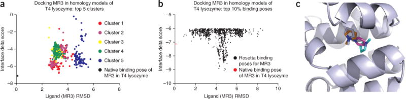
Docking MR3 into comparative models of T4 lysozyme. The MR3 ligand was docked into the ten lowest-energy comparative models of T4 lysozyme, as detailed in Steps 17–22 of the protocol. (a) 10,000 binding modes were clustered by RMSD using applications available in the bcl::Commons. The largest five clusters are shown, with the interface_delta score plotted against the RMSD to the native ligand-binding mode (shown in black). Generally, the largest clusters are also those with the lowest RMSD to the native binding mode. (b) The RMSD between 10,000 binding modes and the native binding mode (shown in red) was computed. The top ten percent of models by interface_delta score are shown here. Sub-angstrom binding modes are within the top ten percent of models, but Rosetta also identifies an alternative lower-energy binding mode within the site. (c) The lowest RMSD binding mode (orange) is closer to the native binding mode (gray) compared with the lowest-energy binding mode of the largest cluster (magenta) and the lowest-energy binding mode overall (cyan).

The appropriate RMSD cutoff for clustering will vary depending on the characteristics of the protein-binding site and the ligand being docked. In this example, owing to the ligand size, a conservative cluster RMSD cutoff of 2 Å was used. If larger ligands are used, the cluster cutoff can be increased to 3–5 Å (ref. 68). To determine the size of the cluster RMSD cutoff, multiple RMSD values should be tested. Once the clusters have been generated, the cluster sizes (i.e., the number of models in each cluster) can be measured. If any single cluster contains a large percentage of the total models used, a larger cutoff may be appropriate.

In addition to clustering ligands, experimental data can be used to determine the correct ligand-binding mode. Kaufmann et al.¹⁸ used the relative rank of ligand energies from analogs of serotonin to determine the binding mode of serotonin into a Rosetta-built comparative model of the human serotonin transporter (hSERT). Experimental binding affinities were correlated to the rank of each small molecule in the binding pocket of hSERT. With the same comparative model, Combs et al.⁶⁸ performed computational mutagenesis of the hSERT binding pocket to determine the binding mode of S- and R-citalopram.

In the example of MR3 docked into a comparative model of T4 lysozyme demonstrated in this tutorial (Supplementary Data), results from Rosetta can be compared with the crystal structure from the PDB. By computing RMSD values between models generated by Rosetta and the experimentally determined or native structure, the accuracy of the models can be evaluated. The methods used to generate these RMSD values can be found in the Supplementary Discussion.

Plotting the interface_delta score versus RMSD of the ligand models, as shown in Figure 5, demonstrates that a local minimum exists in a different binding site from that observed in the native crystal structure. Often, when a small ligand is docked into a large binding pocket, several local energy minima in which the ligand can bind are detected. Rosetta is able to identify alternative binding pockets besides that found in the crystal structure. However, the binding mode closest to that of the crystal structure still ranks within the top 3% of the total docked binding modes. An energy funnel is often observed in score versus RMSD plots, indicating the presence of a single energy minimum. However, the energy funnel in Figure 5 is poorly formed, which is not surprising given the nature of the complex.

The results from the modeling example presented in this protocol point to the challenges associated with docking a small, symmetric ligand into a relatively large binding pocket. Obtaining the correct binding conformation and position of the ligand is further hampered by the low confidence of the comparative model. However, the results also show that Rosetta is capable of sampling the correct binding conformation and assigning this conformation a relatively low energy according to its knowledge-based scoring function. Further, in a situation in which the binding conformation is unknown, Rosetta may be used to predict potential interacting residues. The predicted model will then need to be tested experimentally to confirm its validity.

References

- 1.Rohl CA, Strauss CEM, Misura KMS, Baker D. Protein structure prediction using Rosetta. Methods Enzymol. 2004;383:66–93. doi: 10.1016/S0076-6879(04)83004-0. [DOI] [PubMed] [Google Scholar]
- 2.Siegel JB, et al. Computational design of an enzyme catalyst for a stereoselective bimolecular Diels-Alder reaction. Science. 2010;329:309–313. doi: 10.1126/science.1190239. [DOI] [PMC free article] [PubMed] [Google Scholar]
- 3.Kuhlman B, et al. Design of a novel globular protein fold with atomic-level accuracy. Science. 2003;302:1364–1368. doi: 10.1126/science.1089427. [DOI] [PubMed] [Google Scholar]
- 4.Davis IW, Baker D. RosettaLigand docking with full ligand and receptor flexibility. J Mol Biol. 2009;385:381–392. doi: 10.1016/j.jmb.2008.11.010. [DOI] [PubMed] [Google Scholar]
- 5.Misura KMS, Chivian D, Rohl CA, Kim DE, Baker D. Physically realistic homology models built with ROSETTA can be more accurate than their templates. Proc Natl Acad Sci USA. 2006;103:5361–5366. doi: 10.1073/pnas.0509355103. [DOI] [PMC free article] [PubMed] [Google Scholar]
- 6.Davis IW, Raha K, Head MS, Baker D. Blind docking of pharmaceutically relevant compounds using RosettaLigand. Protein Sci. 2009;18:1998–2002. doi: 10.1002/pro.192. [DOI] [PMC free article] [PubMed] [Google Scholar]
- 7.Das R, Baker D. Macromolecular modeling with Rosetta. Annu Rev Biochem. 2008;77:363–382. doi: 10.1146/annurev.biochem.77.062906.171838. [DOI] [PubMed] [Google Scholar]
- 8.Kaufmann KW, Lemmon GH, Deluca SL, Sheehan JH, Meiler J. Practically useful: what the Rosetta protein modeling suite can do for you. Biochemistry. 2010;49:2987–2998. doi: 10.1021/bi902153g. [DOI] [PMC free article] [PubMed] [Google Scholar]
- 9.Rohl CA, Strauss CEM, Chivian D, Baker D. Modeling structurally variable regions in homologous proteins with Rosetta. Proteins. 2004;55:656–677. doi: 10.1002/prot.10629. [DOI] [PubMed] [Google Scholar]
- 10.Meiler J, Baker D. Coupled prediction of protein secondary and tertiary structure. Proc Natl Acad Sci USA. 2003;100:12105–12110. doi: 10.1073/pnas.1831973100. [DOI] [PMC free article] [PubMed] [Google Scholar]
- 11.Yarov-Yarovoy V, Schonbrun J, Baker D. Multipass membrane protein structure prediction using Rosetta. Proteins. 2006;62:1010–1025. doi: 10.1002/prot.20817. [DOI] [PMC free article] [PubMed] [Google Scholar]
- 12.Bradley P, et al. Free modeling with Rosetta in CASP6. Proteins. 2005;61(suppl. 7):128–134. doi: 10.1002/prot.20729. [DOI] [PubMed] [Google Scholar]
- 13.Bradley P, Misura KMS, Baker D. Toward high-resolution de novo structure prediction for small proteins. Science. 2005;309:1868–1871. doi: 10.1126/science.1113801. [DOI] [PubMed] [Google Scholar]
- 14.Das R, et al. Structure prediction for CASP7 targets using extensive all-atom refinement with Rosetta@home. Proteins. 2007;69(suppl. 8):118–128. doi: 10.1002/prot.21636. [DOI] [PubMed] [Google Scholar]
- 15.Rohl CA. Protein structure estimation from minimal restraints using Rosetta. Methods Enzymol. 2005;394:244–260. doi: 10.1016/S0076-6879(05)94009-3. [DOI] [PubMed] [Google Scholar]
- 16.Lange OF, et al. Determination of solution structures of proteins up to 40 kDa using CS-Rosetta with sparse NMR data from deuterated samples. Proc Natl Acad Sci USA. 2012;109:10873–10878. doi: 10.1073/pnas.1203013109. [DOI] [PMC free article] [PubMed] [Google Scholar]
- 17.Lange OF, Baker D. Resolution-adapted recombination of structural features significantly improves sampling in restraint-guided structure calculation. Proteins. 2012;80:884–895. doi: 10.1002/prot.23245. [DOI] [PMC free article] [PubMed] [Google Scholar]
- 18.Kaufmann KW, et al. Structural determinants of species-selective substrate recognition in human and Drosophila serotonin transporters revealed through computational docking studies. Proteins. 2009;74:630–642. doi: 10.1002/prot.22178. [DOI] [PMC free article] [PubMed] [Google Scholar]
- 19.Lees-Miller JP, et al. Interactions of H562 in the S5 helix with T618 and S621 in the pore helix are important determinants of hERG1 potassium channel structure and function. Biophys J. 2009;96:3600–3610. doi: 10.1016/j.bpj.2009.01.028. [DOI] [PMC free article] [PubMed] [Google Scholar]
- 20.Keeble AH, et al. Experimental and computational analyses of the energetic basis for dual recognition of immunity proteins by colicin endonucleases. J Mol Biol. 2008;379:745–759. doi: 10.1016/j.jmb.2008.03.055. [DOI] [PubMed] [Google Scholar]
- 21.Fortenberry C, et al. Exploring symmetry as an avenue to the computational design of large protein domains. J Am Chem Soc. 2011;133:18026–18029. doi: 10.1021/ja2051217. [DOI] [PMC free article] [PubMed] [Google Scholar]
- 22.Eswar N, Eramian D, Webb B, Shen MY, Sali A. Protein structure modeling with MODELLER. Methods Mol Biol. 2008;426:145–159. doi: 10.1007/978-1-60327-058-8_8. [DOI] [PubMed] [Google Scholar]
- 23.Perola E, Walters WP, Charifson PS. A detailed comparison of current docking and scoring methods on systems of pharmaceutical relevance. Proteins. 2004;56:235–249. doi: 10.1002/prot.20088. [DOI] [PubMed] [Google Scholar]
- 24.Carlsson J, et al. Ligand discovery from a dopamine D3 receptor homology model and crystal structure. Nat Chem Biol. 2011;7:769–778. doi: 10.1038/nchembio.662. [DOI] [PMC free article] [PubMed] [Google Scholar]
- 25.Ballester PJ, Westwood I, Laurieri N, Sim E, Richards WG. Prospective virtual screening with Ultrafast Shape Recognition: the identification of novel inhibitors of arylamine N-acetyltransferases. J R Soc Interface. 2010;7:335–342. doi: 10.1098/rsif.2009.0170. [DOI] [PMC free article] [PubMed] [Google Scholar]
- 26.Schneider G, Fechner U. Computer-based de novo design of drug-like molecules. Nat Rev Drug Discov. 2005;4:649–663. doi: 10.1038/nrd1799. [DOI] [PubMed] [Google Scholar]
- 27.Schneider G, et al. Voyages to the (un)known: adaptive design of bioactive compounds. Trends Biotechnol. 2009;27:18–26. doi: 10.1016/j.tibtech.2008.09.005. [DOI] [PubMed] [Google Scholar]
- 28.Meiler J, Baker D. ROSETTALIGAND: protein-small molecule docking with full side-chain flexibility. Proteins. 2006;65:538–548. doi: 10.1002/prot.21086. [DOI] [PubMed] [Google Scholar]
- 29.Lemmon G, Meiler J. Rosetta Ligand docking with flexible XML protocols. Methods Mol Biol. 2012;819:143–155. doi: 10.1007/978-1-61779-465-0_10. [DOI] [PMC free article] [PubMed] [Google Scholar]
- 30.Laskowski RA. SURFNET: a program for visualizing molecular surfaces, cavities, and intermolecular interactions. J Mol Graph. 1995;13:323–330. doi: 10.1016/0263-7855(95)00073-9. [DOI] [PubMed] [Google Scholar]
- 31.Huang B, Schroeder M. LIGSITEcsc: predicting ligand binding sites using the Connolly surface and degree of conservation. BMC Struct Biol. 2006;6:19. doi: 10.1186/1472-6807-6-19. [DOI] [PMC free article] [PubMed] [Google Scholar]
- 32.Kalidas Y, Chandra N. PocketDepth: a new depth-based algorithm for identification of ligand binding sites in proteins. J Struct Biol. 2008;161:31–42. doi: 10.1016/j.jsb.2007.09.005. [DOI] [PubMed] [Google Scholar]
- 33.Dunbrack RL, Karplus M. Backbone-dependent rotamer library for proteins. Application to side-chain prediction. J Mol Biol. 1993;230:543–574. doi: 10.1006/jmbi.1993.1170. [DOI] [PubMed] [Google Scholar]
- 34.Li Z, Scheraga HA. Monte Carlo-minimization approach to the multiple-minima problem in protein folding. Proc Natl Acad Sci USA. 1987;84:6611–6615. doi: 10.1073/pnas.84.19.6611. [DOI] [PMC free article] [PubMed] [Google Scholar]
- 35.Simons KT, Kooperberg C, Huang E, Baker D. Assembly of protein tertiary structures from fragments with similar local sequences using simulated annealing and Bayesian scoring functions. J Mol Biol. 1997;268:209–225. doi: 10.1006/jmbi.1997.0959. [DOI] [PubMed] [Google Scholar]
- 36.Metropolis N, Rosenbluth AW, Rosenbluth MN, Teller AH, Teller E. Equation of state calculations by fast computing machines. J Chem Phys. 1953;21:1087. [Google Scholar]
- 37.Rarey M, Kramer B, Lengauer T, Klebe G. A fast flexible docking method using an incremental construction algorithm. J Mol Biol. 1996;261:470–489. doi: 10.1006/jmbi.1996.0477. [DOI] [PubMed] [Google Scholar]
- 38.Verdonk ML, Cole JC, Hartshorn MJ, Murray CW, Taylor RD. Improved protein-ligand docking using GOLD. Proteins. 2003;52:609–623. doi: 10.1002/prot.10465. [DOI] [PubMed] [Google Scholar]
- 39.Friesner RA, et al. Glide: a new approach for rapid, accurate docking and scoring. 1. Method and assessment of docking accuracy. J Med Chem. 2004;47:1739–1749. doi: 10.1021/jm0306430. [DOI] [PubMed] [Google Scholar]
- 40.Ewing TJ, Makino S, Skillman AG, Kuntz ID. DOCK 4.0: search strategies for automated molecular docking of flexible molecule databases. J Comput Aided Mol Des. 2001;15:411–428. doi: 10.1023/a:1011115820450. [DOI] [PubMed] [Google Scholar]
- 41.Gohlke H, Hendlich M, Klebe G. Knowledge-based scoring function to predict protein-ligand interactions. J Mol Biol. 2000;295:337–356. doi: 10.1006/jmbi.1999.3371. [DOI] [PubMed] [Google Scholar]
- 42.Kaufmann KW, Meiler J. Using RosettaLigand for small molecule docking into comparative models. PLoS ONE. 2012;7:e50769. doi: 10.1371/journal.pone.0050769. [DOI] [PMC free article] [PubMed] [Google Scholar]
- 43.Mobley DL, et al. Predicting absolute ligand binding free energies to a simple model site. J Mol Biol. 2007;371:1118–1134. doi: 10.1016/j.jmb.2007.06.002. [DOI] [PMC free article] [PubMed] [Google Scholar]
- 44.Mooers BHM, Matthews BW. Extension to 2268 atoms of direct methods in the ab initio determination of the unknown structure of bacteriophage P22 lysozyme. Acta Crystallogr D Biol Crystallogr. 2006;62:165–176. doi: 10.1107/S0907444905037212. [DOI] [PubMed] [Google Scholar]
- 45.Altschul SF, et al. Gapped BLAST and PSI-BLAST: a new generation of protein database search programs. Nucleic Acids Res. 1997;25:3389–3402. doi: 10.1093/nar/25.17.3389. [DOI] [PMC free article] [PubMed] [Google Scholar]
- 46.Zhang Z, et al. Protein sequence similarity searches using patterns as seeds. Nucleic Acids Res. 1998;26:3986–3990. doi: 10.1093/nar/26.17.3986. [DOI] [PMC free article] [PubMed] [Google Scholar]
- 47.Söding J, Biegert A, Lupas AN. The HHpred interactive server for protein homology detection and structure prediction. Nucleic Acids Res. 2005;33:W244–W248. doi: 10.1093/nar/gki408. [DOI] [PMC free article] [PubMed] [Google Scholar]
- 48.Eddy SR. A new generation of homology search tools based on probabilistic inference. Genome Inform. 2009;23:205–211. [PubMed] [Google Scholar]
- 49.Eddy SR. Accelerated profile HMM searches. PloS Comput Biol. 2011;7:e1002195. doi: 10.1371/journal.pcbi.1002195. [DOI] [PMC free article] [PubMed] [Google Scholar]
- 50.Kelley LA, Sternberg MJE. Protein structure prediction on the Web: a case study using the Phyre server. Nat Protoc. 2009;4:363–371. doi: 10.1038/nprot.2009.2. [DOI] [PubMed] [Google Scholar]
- 51.Canutescu AA, Dunbrack RL. Cyclic coordinate descent: a robotics algorithm for protein loop closure. Protein Sci. 2003;12:963–972. doi: 10.1110/ps.0242703. [DOI] [PMC free article] [PubMed] [Google Scholar]
- 52.Mandell DJ, Coutsias EA, Kortemme T. Sub-angstrom accuracy in protein loop reconstruction by robotics-inspired conformational sampling. Nat Methods. 2009;6:551–552. doi: 10.1038/nmeth0809-551. [DOI] [PMC free article] [PubMed] [Google Scholar]
- 53.Coutsias EA, Seok C, Jacobson MP, Dill KA. A kinematic view of loop closure. J Comput Chem. 2004;25:510–528. doi: 10.1002/jcc.10416. [DOI] [PubMed] [Google Scholar]
- 54.Gront D, Kulp DW, Vernon RM, Strauss CEM, Baker D. Generalized fragment picking in Rosetta: design, protocols and applications. PLoS ONE. 2011;6:e23294. doi: 10.1371/journal.pone.0023294. [DOI] [PMC free article] [PubMed] [Google Scholar]
- 55.Wang G, Dunbrack RL. PISCES: a protein sequence culling server. Bioinformatics. 2003;19:1589–1591. doi: 10.1093/bioinformatics/btg224. [DOI] [PubMed] [Google Scholar]
- 56.Leaver-Fay A, Kuhlman B, Snoeyink J. Rotamer-pair energy calculations using a trie data structure. Lect Notes Comput Sci. 2005;3692:389–400. [Google Scholar]
- 57.Jones D, Taylor W, Thorton J. A New approach to protein fold recognition. Nature. 1992;358:86–89. doi: 10.1038/358086a0. [DOI] [PubMed] [Google Scholar]
- 58.Raman S, et al. Structure prediction for CASP8 with all-atom refinement using Rosetta. Proteins. 2009;77:89–99. doi: 10.1002/prot.22540. [DOI] [PMC free article] [PubMed] [Google Scholar]
- 59.Hirst SJ, Alexander N, McHaourab HS, Meiler J. RosettaEPR: an integrated tool for protein structure determination from sparse EPR data. J Struct Biol. 2011;173:506–514. doi: 10.1016/j.jsb.2010.10.013. [DOI] [PMC free article] [PubMed] [Google Scholar]
- 60.Meiler J, Baker D. The fumarate sensor DcuS: progress in rapid protein fold elucidation by combining protein structure prediction methods with NMR spectroscopy. J Magn Reson. 2005;173:310–316. doi: 10.1016/j.jmr.2004.11.031. [DOI] [PubMed] [Google Scholar]
- 61.Alexander N, Bortolus M, Al-Mestarihi A, Mchaourab H, Meiler J. De novo high-resolution protein structure determination from sparse spin-labeling EPR data. Structure. 2008;16:181–195. doi: 10.1016/j.str.2007.11.015. [DOI] [PMC free article] [PubMed] [Google Scholar]
- 62.DiMaio F, et al. Improved molecular replacement by density- and energy-guided protein structure optimization. Nature. 2011;473:540–543. doi: 10.1038/nature09964. [DOI] [PMC free article] [PubMed] [Google Scholar]
- 63.Shen Y, et al. De novo structure generation using chemical shifts for proteins with high-sequence identity but different folds. Protein Sci. 2010;19:349–356. doi: 10.1002/pro.303. [DOI] [PMC free article] [PubMed] [Google Scholar]
- 64.Herzog F, et al. Structural probing of a protein phosphatase 2A network by chemical cross-linking and mass spectrometry. Science. 2012;337:1348–1352. doi: 10.1126/science.1221483. [DOI] [PubMed] [Google Scholar]
- 65.Grishaev A, Guo L, Irving T, Bax A. Improved fitting of solution X-ray scattering data to macromolecular structures and structural ensembles by explicit water modeling. J Am Chem Soc. 2010;132:15484–15486. doi: 10.1021/ja106173n. [DOI] [PMC free article] [PubMed] [Google Scholar]
- 66.Pandit D, et al. Mapping of discontinuous conformational epitopes by amide hydrogen/deuterium exchange mass spectrometry and computational docking. J Mol Recognit. 2012;25:114–124. doi: 10.1002/jmr.1169. [DOI] [PubMed] [Google Scholar]
- 67.Rathmann D, et al. Ligand-mimicking receptor variant discloses binding and activation mode of prolactin-releasing peptide. J Biol Chem. 2012;287:32181–32194. doi: 10.1074/jbc.M112.349852. [DOI] [PMC free article] [PubMed] [Google Scholar]
- 68.Combs S, Kaufmann K, Field JR, Bakely RD, Meiler J. Y95 and E444 interaction required for high-affinity S-citalopram binding in the human serotonin transporter. ACS Chem Neurosci. 2011;2:75–81. doi: 10.1021/cn100066p. [DOI] [PMC free article] [PubMed] [Google Scholar]
- 69.Nannemann DP, Kaufmann KW, Meiler J, Bachmann BO. Design and directed evolution of a dideoxy purine nucleoside phosphorylase. Protein Eng Des Sel. 2010;23:607–616. doi: 10.1093/protein/gzq033. [DOI] [PMC free article] [PubMed] [Google Scholar]
- 70.Leach AR, Shoichet BK, Peishoff CE. Prediction of protein-ligand interactions. Docking and scoring: successes and gaps. J Med Chem. 2006;49:5851–5855. doi: 10.1021/jm060999m. [DOI] [PubMed] [Google Scholar]
- 71.Smith JA, Vanoye CG, George AL, Meiler J, Sanders CR. Structural models for the KCNQ1 voltage-gated potassium channel. Biochemistry. 2007;46:14141–14152. doi: 10.1021/bi701597s. [DOI] [PMC free article] [PubMed] [Google Scholar]
- 72.Larkin MA, et al. Clustal W and Clustal X version 2.0. Bioinformatics. 2007;23:2947–2948. doi: 10.1093/bioinformatics/btm404. [DOI] [PubMed] [Google Scholar]
- 73.Pettersen EF, et al. UCSF Chimera–a visualization system for exploratory research and analysis. J Comput Chem. 2004;25:1605–1612. doi: 10.1002/jcc.20084. [DOI] [PubMed] [Google Scholar]
- 74.Ward JJ, McGuffin LJ, Buxton BF, Jones DT. Secondary structure prediction with support vector machines. Bioinformatics. 2003;19:1650–1655. doi: 10.1093/bioinformatics/btg223. [DOI] [PubMed] [Google Scholar]
- 75.Leman JK, Koehler J, Mueller R, Karakas M, Woetzel N, Meiler J. Simultaneous prediction of protein secondary structure and transmembrane spans. Proteins. 2013 Apr 10; doi: 10.1002/prot.24258. http://dx.doi.org/10.1002/prot.24258. [DOI] [PMC free article] [PubMed]
- 76.Wang C, Bradley P, Baker D. Protein-protein docking with backbone flexibility. J Mol Biol. 2007;373:503–519. doi: 10.1016/j.jmb.2007.07.050. [DOI] [PubMed] [Google Scholar]
- 77.Qian B, et al. High-resolution structure prediction and the crystallographic phase problem. Nature. 2007;450:259–264. doi: 10.1038/nature06249. [DOI] [PMC free article] [PubMed] [Google Scholar]
- 78.Lemmon G, Kaufmann K, Meiler J. Prediction of HIV-1 protease/inhibitor affinity using RosettaLigand. Chem Biol Drug Des. 2012;79:888–896. doi: 10.1111/j.1747-0285.2012.01356.x. [DOI] [PMC free article] [PubMed] [Google Scholar]
- 79.Humphrey W, Dalke A, Schulten K. VMD: visual molecular dynamics. J Mol Graph. 1996;14:33–38. doi: 10.1016/0263-7855(96)00018-5. [DOI] [PubMed] [Google Scholar]
- 80.Wass MN, Kelley LA, Sternberg MJE. 3DLigandSite: predicting ligand-binding sites using similar structures. Nucleic Acids Res. 2010;38:W469–W473. doi: 10.1093/nar/gkq406. [DOI] [PMC free article] [PubMed] [Google Scholar]
- 81.Morris GM, et al. AutoDock4 and AutoDockTools4: automated docking with selective receptor flexibility. J Comput Chem. 2009;30:2785–2791. doi: 10.1002/jcc.21256. [DOI] [PMC free article] [PubMed] [Google Scholar]
- 82.Case DA, et al. The Amber biomolecular simulation programs. J Comput Chem. 2005;26:1668–1688. doi: 10.1002/jcc.20290. [DOI] [PMC free article] [PubMed] [Google Scholar]
- 83.Alexander N, Woetzel N, Meiler J. Bcl::Cluster: A method for clustering biological molecules coupled with visualization in the Pymol molecular graphics system; Computational Advances in Bio and Medical Sciences (ICCABS), 2011 IEEE 1st International Conference on; 13–18; 2011. [DOI] [PMC free article] [PubMed] [Google Scholar]
- 84.Dunbrack RL, Cohen FE. Bayesian statistical analysis of protein side-chain rotamer preferences. Protein Sci. 1997;6:1661–1681. doi: 10.1002/pro.5560060807. [DOI] [PMC free article] [PubMed] [Google Scholar]
- 85.Simons KT, et al. Improved recognition of native-like protein structures using a combination of sequence-dependent and sequence-independent features of proteins. Proteins. 1999;34:82–95. doi: 10.1002/(sici)1097-0134(19990101)34:1<82::aid-prot7>3.0.co;2-a. [DOI] [PubMed] [Google Scholar]
- 86.Kuhlman B, Baker D. Native protein sequences are close to optimal for their structures. Proc Natl Acad Sci USA. 2000;97:10383–10388. doi: 10.1073/pnas.97.19.10383. [DOI] [PMC free article] [PubMed] [Google Scholar]
- 87.Neria E, Fischer S, Karplus M. Simulation of activation free energies in molecular systems. J Chem Phys. 1996;105:1902–1921. [Google Scholar]
- 88.Lazaridis T, Karplus M. Effective energy function for proteins in solution. Proteins. 1999;35:133–152. doi: 10.1002/(sici)1097-0134(19990501)35:2<133::aid-prot1>3.0.co;2-n. [DOI] [PubMed] [Google Scholar]
- 89.Gordon DB, Marshall SA, Mayo SL. Energy functions for protein design. Curr Opin Struct Biol. 1999;9:509–513. doi: 10.1016/s0959-440x(99)80072-4. [DOI] [PubMed] [Google Scholar]
- 90.Wedemeyer WJ, Baker D. Efficient minimization of angle-dependent potentials for polypeptides in internal coordinates. Proteins. 2003;53:262–272. doi: 10.1002/prot.10525. [DOI] [PubMed] [Google Scholar]
- 91.Ramachandran GN, Ramakrishnan C, Sasisekharan V. Stereochemistry of polypeptide chain configurations. J Mol Biol. 1963;7:95–99. doi: 10.1016/s0022-2836(63)80023-6. [DOI] [PubMed] [Google Scholar]
- 92.Fleishman SJ, et al. RosettaScripts: a scripting language interface to the Rosetta macromolecular modeling suite. PLoS ONE. 2011;6:e20161. doi: 10.1371/journal.pone.0020161. [DOI] [PMC free article] [PubMed] [Google Scholar]
Associated Data
This section collects any data citations, data availability statements, or supplementary materials included in this article.