

SUMMARY
While genes are defined by sequence, in biological systems a protein’s function is largely determined by its three-dimensional structure. Evolutionary information embedded within multiple sequence alignments provides a rich source of data for inferring structural constraints on macromolecules. Still, many proteins of interest lack sufficient numbers of related sequences, leading to noisy, error-prone residue-residue contact predictions. Here we introduce DeepContact, a convolutional neural network (CNN)-based approach that discovers co-evolutionary motifs and leverages these patterns to enable accurate inference of contact probabilities, particularly when few related sequences are available. DeepContact significantly improves performance over previous methods, including in the CASP12 blind contact prediction task where we achieved top performance with another CNN-based approach. Moreover, our tool converts hard-to-interpret coupling scores into probabilities, moving the field toward a consistent metric to assess contact prediction across diverse proteins. Through substantially improving the precision-recall behavior of contact prediction, DeepContact suggests we are near a paradigm shift in template-free modeling for protein structure prediction.
In Brief
Many protein structures of interest remain out of reach for both computational prediction and experimental determination. DeepContact learns patterns of coevolution across thousands of experimentally determined structures, identifying conserved local motifs and leveraging this information to improve protein residue-residue contact predictions. DeepContact extracts additional information from the evolutionary couplings using its knowledge of co-evolution and structural space, while also converting coupling scores into probabilities that are comparable across protein sequences and alignments.
INTRODUCTION
Protein structure and function are by nature intertwined, with structure, or structural properties, playing a large role in defining function. As such, ever since the X-ray structure of lysozyme led to the elucidation of its mechanism of catalytic action, determining protein structure has been one of the most important challenges in biology (Phillips, 1966; Phillips, 1967). In parallel, given the many obstacles to experimental structure determination, computational prediction of protein structure remains one of the longest-standing challenges in computational biology (Moult et al., 2014, 2016). Existing approaches to protein structure prediction can be categorized into two types: template-based modeling and template-free modeling. With the requirement of a homologous structure, template-based methods are often not applicable to structure prediction tasks of interest, including orphan proteins, and thus for many novel proteins the field has turned to template-free, or de novo, folding approaches that predict 3D structures using the query sequence alone (Zhang, 2008; Xu and Zhang, 2012). While these approaches work reasonably well for smaller proteins, they have generally required further difficult-to-obtain experimental data for larger proteins (Bradley et al., 2005; Moult et al., 2014, 2016).
Recent computational advances, together with the availability of large protein sequence databases, have enabled us to exploit rich evolutionary information encoded within multiple sequence alignments (MSAs) to assist traditional protein structure prediction approaches. Notably, evolutionary coupling analysis methods, such as direct-coupling analysis, GREMLIN, (meta-) PSICOV, and EVFold, take an MSA as input and predict residue-residue contacts by learning an inherent graphical model structure that incorporates pairwise terms to capture evolutionary constraints among residues (Ekeberg et al., 2013; Morcos et al., 2011; Kamisetty et al., 2013; Jones et al., 2012, 2015; Marks et al., 2011; Kaján et al., 2014). Several tools (including Rosetta) have successfully incorporated evolutionary couplings into their pipelines as distance restraints to significantly improve predictions, particularly for proteins that have proven challenging using traditional approaches (Ovchinnikov et al., 2015, 2017). In addition, evolutionary coupling-based methods have been successfully applied to protein complex assembly and interactions, disordered region structure prediction, RNA structure prediction, and mutagenesis analysis (Ovchinnikov et al., 2014; Uguzzoni et al., 2017; Hopf et al., 2014, 2017; Toth-Petroczy et al., 2016; De Leonardis et al., 2015; Weinreb et al., 2016).
Despite these advances, state-of-the-art evolutionary coupling approaches still have several major failings that limit their applicability. First, they require large, high-quality MSAs and often generate sparse or poor contact predictions for proteins with less robust MSAs (Moult et al., 2016). Second, the units of evolutionary couplings are arbitrary; while there have been recent attempts to define significant couplings, for the most part users are left to decide how many couplings to take as true distances restraints (Toth-Petroczy et al., 2016). Third, these methods do not put any outside constraints, beyond sparsity of contacts through the use of regularization, on the coupling matrix, ignoring everything we know about protein structures.
Deep learning continues to develop as a powerful set of tools for solving an increasingly diverse range of problems, including many related to biological systems (LeCun et al., 2015; Zhou and Troyanskaya, 2015; Angermueller et al., 2016; Wang et al., 2017). The key insights of modern machine learning include both the power of automatic feature selection and the ability to integrate data sources, as well as the ability to leverage and encode contextual data and to convert inputs of arbitrary units into well-calibrated probabilities (Cho et al., 2016; Jones et al., 2015; Gao et al., 2017; Niculescu-Mizil and Caruana, 2005). While the proliferation of biological data has made many tasks suitable for deep learning, biology, perhaps more than many other fields grappling with expanding amounts of data, often seeks understanding as much as improved inference. Therefore, powerful deep-learning approaches in biology hold the promise of not only having superior predictive performance over previous methods, but also of including a focus on interpretability allowing insights into the underlying dynamics and mechanisms of the biological phenomena at play.
Here we introduce DeepContact, an approach that employs a convolutional neural network (CNN) to learn structural interaction motifs from thousands of proteins with experimentally solved structures. Taking raw evolutionary couplings produced by existing methods (e.g., CCMPred) as input, we trained the network to predict contact maps using experimentally determined structures (Seemayer et al., 2014). DeepContact automatically and effectively leverages local information and multiple features to discover patterns in contact map space and embeds this knowledge within the neural network. Notably, few CNN layers suffice, avoiding the potential for overtraining and allowing the model to be trained on a large number of structures in a reasonable amount of time.
For subsequent prediction of new proteins, DeepContact uses what it has learned about structure and contact map space to impute missing contacts and remove spurious predictions, leading to significantly more accurate inference of residue-residue contacts. Its performance on several benchmark datasets and in the most recent Critical Assessment of protein Structure Prediction, CASP12, demonstrates DeepContact’s (also known as iFold_1 in the CASP12 results) significant improvement over previous evolutionary coupling analyses, which do not take contact or structure space into account (Moult et al., 2016; CASP12).
Notably, DeepContact automatically converts coupling scores into probabilities, such that the values have common scale across proteins and alignments, simplifying their use and interpretation. Moreover, it identifies patterns that capture a set of “rules” for structural motif interactions.
Given the improved precision-recall characteristics and associated probabilities, downstream folding methods based on DeepContact have the potential to significantly improve structure prediction by maximizing the probabilities of the satisfied restraints. DeepContact not only makes many proteins with hard-to-predict structures accessible to evolutionary coupling analysis, but it also provides a rich resource for further evolutionary analysis of protein sequence and structure.
RESULTS
Overview of DeepContact
Observing the contact maps resulting from solved experimental structures (a contact is defined as when two residues in the structure are within a distance d of each other), distinctive patterns emerge whereby one can identify structural components such as parallel and antiparallel β sheets as well as helix-helix interactions (Hu et al., 2002). Not all sets of contact maps are equally likely to emerge from a protein structure, and contextual information can help inform our confidence in a particular contact. In the image recognition field, CNNs have proven very effective at taking a noisy image and returning the clean image (Zhang et al., 2017). We pursue the intuition that by training a CNN to predict contact probabilities using evolutionary couplings and experimentally solved structures, the CNN is able to learn about contact map space. Using multiple convolutional layers our algorithm, DeepContact, effectively re-weights evolutionary couplings based on the contextual information of the contact map, down-weighting contacts that are unlikely to be true given the context and the space of evolutionary couplings and up-weighting contacts in the reverse case.
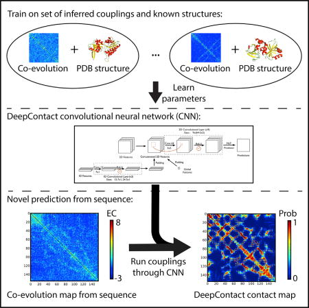
The DeepContact framework consists of a CNN that takes evolutionary couplings as input and predicts a probability of contact for each pair of residues (Figure 1A). After obtaining the input features, e.g., evolutionary couplings from CCMPred, they are fed into the fully convolutional neural network which extracts multiple levels of features by successively applying a convolutional layer, a batch normalization layer, and a rectified linear unit layer (Seemayer et al., 2014). DeepContact then uses a shared-weight neural network to compute the final contact probability for each pair of residues (Figure 1A). To balance predictive performance, ease of training, and interpretation, DeepContact uses nine-convolutional layers. DeepContact was trained on the solved structures from the 40% filtered ASTRAL SCOPe 2.06 dataset split according to the ratio 8:1:1 as training:validation:test (Figure 1B) (Fox et al., 2013). This was done such that members in a superfamily did not appear in both the training and testing sets, ensuring that proteins in the testing set share at most the class and fold with any protein in the training or validation set and that we did not train on structures in our test set.
Figure 1. Overview of DeepContact.

(A) Structure of the full-feature DeepContact model. DeepContact takes in global, 1D, and 2D features calculated from the amino acid sequence, including evolutionary couplings, and uses a CNN to predict contacts.
(B) DeepContact trains using a set of solved structures, taking in the distance matrix (left) and, as a preprocessing step, producing a contact matrix using an 8 Å threshold (right). Intrinsically, these contact maps have patterns, and clearly some matrices cannot be contact maps. By learning the structure of contact matrices and the relationship between couplings and contacts, DeepContact is able to vastly improve evolutionary- based contact prediction.
We trained using a cross-entropy loss function adapted to deal with the imbalance in the dataset by weighting positive and negative examples equally. We trained an additional model including sequence features (precisely, predicted secondary structure, predicted solvent accessibility, and column-wise amino acid frequencies) and global features (i.e., number of effective sequences, Neff) in addition to pairwise features (STAR Methods) (Seemayer et al., 2014; Altschul et al., 1997). Importantly, all of these features are derived from the underlying sequence. Whereas raw evolutionary couplings are computed using a global model that does not know anything about contact map space, DeepContact effectively learns about protein structure and contact map space from the thousands of examples it has previously seen, leveraging this information by integrating contextual information to improve predictions (Figure 1B).
Improved Contact Prediction
Evolutionary couplings have emerged as a powerful tool for the prediction of protein structures, particularly for hard-to-predict structures such as membrane proteins and orphan proteins (Hopf et al., 2012; Marks et al., 2011; Toth-Petroczy et al., 2016). The goal is to determine residues that are close in 3D space, with the underlying assumption that the columns of an MSA that are highly coupled but far in chain distance will be close in the folded structure (Morcos et al., 2011). The improvement in evolutionary couplings for contact prediction has been driven by the use of global statistical models that infer direct, as opposed to transitive, evolutionary couplings by effectively conditioning on the rest of the alignment (Morcos et al., 2011; Ekeberg et al., 2013). Sparsity of contacts is enforced through regularization; however, these methods are oblivious to the space of possible contact maps. Generally, users take the top L/x (where L is the length of the protein and x is an integer) medium- or long-range (defined by a separation in chain distance) evolutionary couplings to be the predicted contacts.
We evaluated the performance of DeepContact on the ASTRAL validation set (660 proteins), on a set of 228 previous CASP targets (CASP228), on a set of 220 CAMEO targets, and by participating in the blind prediction tasks from the well-established CASP12 experiment (Fox et al., 2013; Moult et al., 2014, 2016; Haas et al., 2013). For medium- and long-range contacts (residues 12 apart or more in chain distance) we substantially outperformed the baseline of CCMPred across the precision/recall curve on all three of our validation sets after training the model using CCMPred evolutionary couplings as the only input features (Figures 2A–2C).
Figure 2. Improved Performance of DeepContact on Benchmark Datasets.
(A) DeepContact outperforms CCMPred on the ASTRAL validation set using only CCMPred as features. Including other features further improves the precision-recall performance.
(B) Precision-recall performance of contact-prediction methods on the CAMEO dataset. DeepContact further outperforms metaPSICOV on the CAMEO dataset.
(C) Precision-recall performance of contact-prediction methods on the CASP228 dataset. On all three validation sets, using our novel probability cutoff enables enhancement of the precision/recall characteristics of DeepContact. Effectively, we exclude sequences or contacts with little confidence, and include contacts in which we have more confidence, leading to improved performance.
(D) The improved contact-prediction performance of DeepContact over CCMPred leads to improved contact-assisted folding across the CASP12 free-modeling target set. Targets where folding failed using CCMPred contacts are plotted at a TM-score of 0.
To maximize the predictive performance for the CASP12 experiment, at the expense of interpretation, we incorporated additional input features. These consisted of additional 2D features (precisely, EVFold predictions, mutual information [MI], normalized MI, and mean contact potential), global features (Neff of the alignment and SD of the CCMPred and EVFold predictions), and 1D features (predicted solvent accessibility, predicted secondary structure, and column-wise amino acid frequencies) (STAR Methods). A benefit of deep learning is that, given many input features, it is able to learn which features, and interactions between features, are important for prediction while disregarding those that are not. We participated in the CASP12 experiment finishing with the 2nd best average rank across the variety of categories and ranking metrics considered, as well as in the top two methods based on average F1 score, with the other top method, RaptorX-Contact, being another CNN-based model using a much deeper Residual Learning network (CASP12; Wang et al., 2017; Schaarschmidt et al., 2017).
Using an L/2 cutoff for the free-modeling (FM) targets we ranked second in average F1 score for both the set of long-range (≥24 in chain distance) only contacts and for the set of long- and medium-range (≥12 in chain distance) contacts. This was despite the fact that DeepContact earned an F1 score of 0 for one of the 38 FM targets due to a submission script bug that prevented us from submitting. Comparing with the other top method, RaptorX-Contact, on the 37 structures where we both submitted predictions, RaptorX-Contact slightly outperformed on the combined set of long- and medium-range contacts (average F1 score of 20.717 for RaptorX-Contact versus our DeepContact-based method, iFold_1, average F1 score of 20.011), while we slightly outperformed on the long-range-only contacts (average F1 score of 20.233 for RaptorX-Contact versus our average F1 score of 20.775) (Wang et al., 2017). DeepContact also outperformed on the long-range contacts for the FM/template-based modeling (TBM) targets using an L/2 cutoff. Despite only submitting 54/57 targets for the joint set of FM and FM/TBM targets due to the submission script bug, DeepContact achieved an experiment best overall average F1 score, including 0 for the 3 missed targets, of 23.226 (iFold_1) with MetaPSICOV (Jones et al., 2015) the next best non-DeepContact-based method, submitting 57/57 targets for an average F1 score of 22.470 (Deepfold-Contact is an earlier version of DeepContact submitted in parallel, see STAR Methods) (CASP12). Notably, folding using contacts generally requires L/2 or more contacts for a quality structure, making L/2 a relevant cutoff for downstream structure prediction (Marks et al., 2011).
On our three benchmark datasets, DeepContact substantially outperforms CCMPred on medium- and long-range contacts (residue-residue pairs separated by more than 12 in chain distance) across the entire precision-recall curve from L/10 all the way to 20*L (Figures 2A–2C). This is true for the simplest version of DeepContact trained using CCMPred as the only feature (green line in Figures 2A–2C), demonstrating the power of the underlying convolutional model to extract additional information from the CCMPred-predicted evolutionary couplings. Including the full-set of additional features (STAR Methods) further enhances the performance of DeepContact (blue line in Figures 2A–2C). On the two more challenging datasets, CASP228 and CAMEO, we also compared DeepContact with the previous state-of-the-art method metaPSICOV and again significantly outperformed using the full-featured model (Figures 2B and 2C). metaPSICOV is a machine-learning method that uses the same general features as DeepContact; for all overlapping features we used the same inputs, demonstrating the power of the CNN-based approach (Jones et al., 2015).
To demonstrate that the improved precision-recall behavior leads to improved structure prediction, we used the top L predictions from DeepContact and CCMPred to fold the 36 FM targets from CASP12 with released coordinates. We ran an off-the-shelf folding algorithm, Confold, without any further refinement and selected the top 5 of 500 models by energy for each target (Adhikari et al., 2015). We calculated the TM-score, a measure of similarity between protein structures, for these top models and for each target compared the maximum TM-score using the DeepContact predictions with the maximum TM-score using the CCMPred predictions; in every case DeepContact improved the TM-score with an average improvement of 0.15 excluding the 8/36 targets where Confold failed using the CCMPred contacts (Zhang and Skolnick, 2005). On these challenging targets, whereas 8/36 targets failed and 0/36 targets had a TM-score above 0.3 for the CCMPred contacts, 25/36, 12/36, and 4/36 targets had a TM-score above 0.3, 0.4, and 0.5, respectively, using DeepContact’s predicted contacts representing a significant improvement (Figure 2D) (Xu and Zhang, 2010).
A demonstrative example, PDB: 3LRT, shows how DeepContact, using both the CCMPred-only model and the full-feature model, is able to integrate over the local context to improve contact predictions (Figure 3) (Cherney et al., 2011). The diffuse patterns of couplings from CCMPred lead to suboptimal predictions; however, DeepContact is able to integrate across these regions to improve contact prediction (Figure 3). The Neff score of the MSA input for PDB: 3LRT was in line with the rest of the set at 8.0, compared with an average of 8.3 for our training set, 8.7 for the ASTRAL test set, 6.4 for the CASP228 set, and 6.6 for the CAMEO set (higher Neff implies more evolutionary information). Using a cutoff of L/2, the full-featured implementation of DeepContact has a precision of 0.83, while CCMPred has a precision of 0.56 for the 78 predicted contacts. Using a probability cutoff of 0.99 for DeepContact includes an additional 21 contacts, for a total of 99 predicted contacts, while the precision remains 0.83 (Figure S1). DeepContact’s improvement of 0.27 at L/2 is in line with the results across the three benchmark datasets, where DeepContact improves precision by 0.25, 0.19, and 0.24 on average for the ASTRAL validation, CASP228, and CAMEO sets, respectively. In addition, most of DeepContact’s false-positive contacts border a region of true positives, and the two that do not are in fact dimer contacts in the biologically active homodimer (Figure 3A) (Cherney et al., 2011). DeepContact, using only the CCMPred output as a feature, identifies the same regions as DeepContact with the full-feature set, with the full-featured version using the additional features to sharpen the predictions (Figure 3B). Even though the model was trained on the contact maps after thresholding (Figure 1B), the output resembles the full-distance matrix (Figure 3B).
Figure 3. DeepContact Integrates Local Information to Improve Contact Prediction.
(A) Example of how DeepContact (upper right triangle) improves contact prediction over CCMPred (lower left triangle) input for PDB: 3LRT_A (Cherney et al., 2011). Most of the DeepContact “false-positives” border regions of true positives, and the two that do not (black circles) are true homodimer contacts between chain A (green) and chain B (cyan) separated by 3.6 and 4.3 Å, respectively (right panel). See also Figure S1.
(B) DeepContact integrates local information. Using CCMPred as the only input feature (top left), DeepContact is able to identify patterns indicative of secondary structure elements (bottom left). Using additional features sharpens the predicted contact map (top right). These matrices resemble the experimentally determined distance matrix (bottom right).
DeepContact re-orders the entire rank-ordered list of contacts, not just the top contacts from CCMpred, with the ordering of contacts by DeepContact being much closer to the ground-truth ordering by distance in the structure (Figure 4A). Notably, the false-positive contact pairs, as called using a hard distance cutoff of 8 Å, for DeepContact are significantly closer than the false-positive contact pairs of CCMPred (Figure 4B). DeepContact substantially improves contact prediction by training a CNN on thousands of solved structures, which allows it to use knowledge of protein structure space to improve predictions for novel protein structures.
Figure 4. DeepContact Reranks Full Contact Distribution.

(A) Contacts were ranked across the entire ASTRAL validation set based on distance (black), DeepContact probability (blue), and CCMPred score (red). To make CCMPred comparable across examples we normalized to the SD of the medium- and long-range scores within each protein. The x axis is the rank-ordered list of DeepContact probabilities, and the y axis the average distance of the higher-ranked contacts. DeepContact (blue) significantly improves the rank order of contacts across the distribution compared with CCMPred, being much closer to the true rank order of contacts (black).
(B) The average distance of the false positives for each of the ASTRAL validation set structures as called by CCMPred versus as called by DeepContact. The “false positives” called by DeepContact are significantly closer in the experimental structure, with many of them lying just beyond the 8 Å cutoff.
Probabilistic Interpretation of Couplings
Evolutionary coupling scores exist on a poorly defined scale, as they are calculated by taking the maximum entropy solution to the global model for coupling matrices and calculating the Frobenius norm of each coupling matrix after correcting for the effects of column entropy and undersampling by using average product correction (Buslje et al., 2009; Ekeberg et al., 2013). This scale can change based on alignment size, the number of amino acids in the sequence of interest, and regularization parameters, making the values somewhat arbitrary across different proteins, alignments, and model parameters. Traditionally users of these methods rank order the evolutionary couplings, discarding short-range couplings generally defined as residue-residue pairs separated by fewer than six in chain distance, and then define a cutoff as a fraction of L, the number of amino acids in the sequence. The distribution of evolutionary couplings generally consists of a Gaussian centered near 0 and a fat right hand tail for the highly coupled residue pairs (Toth-Petroczy et al., 2016). Most of the highly coupled pairs in the tail are short-range couplings, which fits with the intuition of highly coupled pairs being close in 3D space. Experienced users often use conservative cutoffs or increase the cutoff as a fraction of L until the contact maps begin to look more like noise than signal (Kim et al., 2014). Recently, more principled approaches have been proposed that model the distribution of evolutionary couplings and assign medium- and long-range couplings to the tail based on the probability of coming from the Gaussian or tail distribution, an approach similar to methods previously applied to coiled-coil domain prediction from pairwise residue correlations (Toth-Petroczy et al., 2016; Berger et al., 1995).
One of the benefits of machine-learning approaches is that by defining an appropriate objective function they naturally transform input feature values into probabilistic estimates. DeepContact is trained using a cross-entropy loss function, thereby converting the input evolutionary couplings (and other features for the full model, see STAR Methods) into contact probabilities. This ability allows us to introduce the idea of using a universal probability cutoff to define contacts, given that the probabilities have consistent scale and meaning across different proteins and alignments. It also allows end-users to select the number of couplings based on the estimated probabilities of the couplings instead of using a hard cutoff. With this probability-based approach the network effectively decides on the significant couplings using all of the features in a context-aware manner. Using probabilistic cutoff scores further enhances the precision-recall behavior by allowing more contacts in cases where DeepContact is more certain in the prediction and not making predictions when it is uncertain (Figure 2). In the example discussed above (PDB: 3LRT) we allow 21 additional couplings using a probability cutoff of 0.99 versus L/2, enhancing the recall while still achieving the same precision of 0.83 (Figures 3A and S1) (Cherney et al., 2011).
Downstream folding pipelines (e.g., Confold, CNS, Rosetta) take in the residue-residue contacts predicted by evolutionary coupling methods and treat them as distance restraints, returning the top model structures that maximally satisfy the distance restraints (Adhikari et al., 2015; Brünger et al., 1998; Ovchinnikov et al., 2015). Assigning probabilities to residue-residue couplings allows a more fine-grained approach, whereby downstream folding algorithms can incorporate the probability of the distance restraints satisfied by a structural model. The conversion of evolutionary couplings to meaningful probabilities will facilitate broader use and integration of evolutionary coupling approaches, while aiding structural model determination through the probabilistic view of satisfying restraints.
Ideally these probabilities would be well-calibrated across examples and proteins, accurately reflecting the confidence that DeepContact has in any individual residue-residue pair prediction. Our probabilities are generally overestimates, particularly in the middle of the distribution (Figure 5). Much of this arises from one of the main challenges of our training task: imbalance in the positive and negative classes. To address the imbalance in the dataset we train with half the weight on positive examples and half the weight on negative examples. This choice is exacerbated for long proteins because as the length, L, of a protein grows the number of contacts also grows in proportion to L; however, the number of entries in the contact map grows with L2 (Kim et al., 2014). Thus, the imbalance grows with the length of the protein and we subsequently end up down-weighting false positives more in longer proteins. Training an additional model that takes in output probabilities, length, and Neff (average log entropy of columns) is one solution to output better-calibrated probabilities. Importantly, some of the false contacts identified by DeepContact are true homodimer contacts and others may be true in another conformation, particularly given the small distances between the residues of many of the false contacts (Figures 3A and 4B) (Hopf et al., 2012; Morcos et al., 2011; Toth-Petroczy et al., 2016).
Figure 5. DeepContact Converts Evolutionary Coupling Scores to Coupling Probabilities.

Boxplot of precision of DeepContact with respect to the ASTRAL validation set (y axis) with DeepContact predictions binned by 0.01 probability. Mean (red) and median (blue) precision are shown for each bin; whiskers represent 5th to 95th percentiles. We trained DeepContact using a cross-entropy loss function, which effectively maximizes the ability to distinguish residue pairs less than 8 Å apart from residues more than 8 Å apart. While the probabilities are better calibrated at the ends of the distribution, those in the middle enable an objective understanding of the likely probability of contacts using the output probabilities.
Visualization toward Interpretable Inference
Deep learning is able to take training data and encode the complex feature relationships relevant for the predictive task into the parameters of the final network, embedding the knowledge it has learned within the network. By training the network to predict residue-residue contact probabilities using evolutionary couplings, DeepContact has learned about protein residue-residue contact map space, as well as the relationship between evolutionary coupling space and contact map space, and is able to effectively leverage that information to improve predictions for targets it has never seen before.
Much of the knowledge embedded within the trained CNN is encoded by the filter parameters of the convolutional layers (STAR Methods). By visualizing the filters and the contact map patterns that activate them, we can begin to disentangle the network, revealing the first-layer units that form the basis for the “grammar” of protein contact space (Figure 6). The deeper layers of the network integrate the local motifs captured by the first layer to form more complex hierarchical interactions at a higher level of abstraction.
Figure 6. Visualization of First-Layer Filters.

Visualization of features picked up by the first layer of a DeepContact model trained with CCMPred as the only feature (STAR Methods). We averaged the top 100 activations of each filter across the ASTRAL validation set and used t-stochastic neighbor embedding to reduce the dimensionality (center gray-shaded matrix). Insets (A–F) show the activation patterns of selected filters, as well as the top 5 structural alignments and sequence similarity of the proteins with the top 100 activations. Filters (center) cluster by secondary structure element, spanning from β segments (red, top) to helical/β to helical segments (blue, bottom). The β patterns fit with the alternating contacts of β sheets (A, B, and F) and distinguish between parallel (A and B) and antiparallel (F) sheets. Helical filter (E) shows a grid-pattern separated by three to four residues, matching the rise of a helix.
To visualize the features identified by the network, we computed the activation values of each filter from the first layer on a non-redundant set of proteins from the SCOP database. Averaging the top 100 protein activations for each filter, we find that many of the observed features correspond to conserved motifs, fitting with our intuitions about the evolutionary patterns of secondary structure and tertiary structure elements such as helices, helix-helix interactions, and β sheets (Figure 6, insets A–F). In the case of β sheets there is an alternating lattice pattern (Figure 6, insets A–C), whereas α-helical motifs consist of grid-like couplings separated by three to four residues (the rise of a helix) (Figure 6, inset E) (Branden, 1999). To visualize the space of filters we applied t-stochastic neighbor embedding, a nonlinear dimensionality reduction method that embeds similar points in the high-dimensional space as points close in two dimensions, on the top activations (Maaten and Hinton, 2008). The filters of the first-layer cluster by secondary structure elements, with β sheet motifs and α-helical motifs separated by motifs that consist of the interaction between the two (Figure 6).
DISCUSSION
We have presented DeepContact, a deep-learning-based method to improve structure prediction and elucidate patterns in the co-evolutionary pressures on macromolecules. DeepContact uses contextual information and the knowledge of thousands of experimentally determined structures to improve structure prediction by identifying interaction motifs. We have demonstrated the ability of DeepContact to improve contact prediction, as well as folding. Moreover, our use of CNNs enables us to successfully convert evolutionary couplings (ECs) into more general contact probabilities, which will be of great value to practitioners. The probabilistic interpretation of DeepContact presented here suggests a framework for contact prediction useful for future CASP experiments; one can use a range of probability cutoffs instead of length-based cutoffs, truly incorporating probabilistic estimates. DeepContact significantly improved over the previous state-of-the-art methods on our validation datasets and during the CASP12 experiment achieved top performance in line with RaptorX, another CNN-based approach, which used a residual network architecture consisting of many more layers, making it more difficult and resource intensive to train and more susceptible to overtraining (Wang et al., 2017).
The improved contact predictions of DeepContact led to improved structural prediction on CASP12 targets compared with CCMPred (Figure 2D, STAR Methods). In their recent publication evaluating contact prediction in CASP12, Schaarschmidt et al. (2017) presented analysis in conflict with these results, suggesting that despite DeepContact’s performance on contact prediction it did not result in improved structural prediction. This analysis focused on a small subset of the CASP12 structures where DeepContact’s average precision was significantly below its average precision across the complete dataset; while the performance on these particular sequences is disappointing and suggests room for further improvement, it is not surprising that in cases where the precision of DeepContact’s predictions are low, these contacts do not improve folding. However, critically, these results cannot be extrapolated to the remaining cases where DeepContact outperforms based on precision as the problematic analysis of Schaarschmidt et al. (2017) suggests.
Further, by analyzing the first-layer filters of the network we have demonstrated the underlying motifs of protein structural interaction space and their correspondence to evolutionary patterns. The challenge remains of further understanding how these motifs are combined to determine the higher-order grammar of evolutionary forces driving protein structure and function. By elucidating the different contact map patterns and features corresponding to identified structural features, we may be able to understand the range of evolutionary patterns that are able to constrain structure.
The full contact maps output by DeepContact are significantly cleaner than the contact maps output by CCMPred. Our algorithm increases the contrast, and the fully plotted contact maps output by DeepContact look much more similar to the full-distance matrices, despite the fact that they were trained only on the binary classification of a contact defined by a distance of less than 8 Å. Just as with the probabilities, this suggests a paradigm where we can effectively use much more of the contact matrix to fold proteins in an FM approach. It also suggests that using smarter objective functions we may well be able to extract even more information from ECs. In addition, the failure modes are such that, by looking at the full matrix, we can often immediately identify by eye whether it is a valid contact map or not and what regions of contacts are suspect. This observation suggests room for improvement in that DeepContact should be able to avoid and eliminate these failure modes. Perhaps more importantly, DeepContact extracts much more information about the distances from the ECs. Improved models for folding that are able to use the additional information content will facilitate a paradigm shift in FM protein structure prediction.
STAR*METHODS
Detailed methods are provided in the online version of this paper and include the following:
KEY RESOURCES TABLE
CONTACT FOR REAGENT AND RESOURCE SHARING
- METHOD DETAILS
- DeepContact Framework
- Features
- Implementation Details
- Datasets
- Filter Visualization
- QUANTIFICATION AND STATISTICAL ANALYSIS
- Contacts
- Probabilites
DATA AND SOFTWARE AVAILABILITY
STAR*METHODS
CONTACT FOR REAGENT AND RESOURCE SHARING
Further information and requests for resources and reagents should be directed to and will be fulfilled by the Lead Contact, Jian Peng, jianpeng@illinois.edu, Department of Computer Science, University of Illinois at Urbana-Champaign, Champaign, IL, USA.
METHOD DETAILS
DeepContact Framework
Neural Network
Convolutional Neural Networks (CNNs) have been well established for diverse learning tasks on both one-dimensional sequence data and two-dimensional image data, including pixel level labeling tasks such as image segmentation (LeCun et al., 1998; Krizhevsky et al., 2012; Long et al., 2015). Here we frame contact prediction as a pixel-level labeling task - viewing each amino acid pair as a ‘pixel’ in the evolutionary coupling matrix (the ‘image’) with the task defined as labeling the true contact pairs. The DeepContact CNN takes in the input features, the primary feature being the evolutionary coupling matrix, and predicts a new corrected contact matrix.
We trained two different models - one with the only feature being an evolutionary coupling matrix and the other including the evolutionary coupling matrix and additional features (see ‘Features’ below) - using experimentally determined structures. For the model with additional features we used three different levels of amino acid features: 2d features, which measure the correlation between two amino acids; 1d features, the statistical information for each amino acid; and global features, the overall features across the whole proteins.
Based on the feature maps, our network consists of 9 convolutional layers, each followed by a batch normalization layer and then a rectified-linear unit (ReLU) layer. Each convolutional layer has 32 filters (i.e. features) of size 5×5 and a stride of 1. To make the final predictions, we concatenate the output of the 3rd, 6th, and 9th layers with the original joint features and use a shared weight MLP on each amino acid pair, which can alternatively be viewed as a convolutional layer with both a filter size and stride of 1. As our objective function we use cross-entropy loss.
Features
Alignment Generation
Co-evolution analyses depend on multiple sequence alignments (MSAs). We generated alignments for all sequences with HHBlits with an e-value threshold of 0.001, a pairwise identity cut-off of 0.99 and a minimum coverage of master sequence of 50% (Remmert et al., 2012). HHblits was configured to run 3 iterations. If the alignment returned by HHBlits had fewer than 1000 sequences we used JackHMMER with an e-value threshold of 10 (Remmert et al., 2012; Eddy, 1998). JackHMMER was also configured to run 3 iterations and the same pairwise identity cut-off and minimum coverage criteria were applied. All homology searches were performed on Uniprot_2016_04.
Two-dimensional Features
For the two-dimensional features, we used CCMPred predictions, EVFold predictions, mutual-information (MI), normalized MI, and the mean contact potential. To generate the evolutionary coupling features we ran CCMPred and EVFold using default parameters on the previously-computed multiple sequence alignments (MSAs) (Seemayer et al., 2014; Kaján et al., 2014).
One-dimensional Features
For one-dimensional features we used predicted solvent accessibility as computed by SOLVPRED , predicted secondary structure as predicted by PSIPRED, and column-wise amino acid frequencies (McGuffin et al., 2000). We ran SOLVPRED and PSIPRED with default parameters.
To convert the 1d features into a ‘2d‘ input for DeepContact, we first conducted 1d convolutions on the 1d features to extract higher-level local information. Then the convolved 1d features are converted to 2d features. Namely, for a specific amino acid pair (i,j), we concatenate i’s 1d feature with j’s 1d feature, resulting in a pairwise feature map. For the 1d convolution, we use one layer containing 12 filters of size 7 and one layer with 24 filters of size 5. These parameters were trained simultaneously to the rest of the DeepContact parameters.
Global Features
For global features, in each case we included the average log entropy of the columns of the MSA (Neff) and the standard deviation of the CCMPred and EVfold predictions. We converted global features by padding them to an L by L matrix.
Combining Features
We concatenated all of the transformed LxL features into an LxLxN matrix, where N is the number of features, and the 2D convolutions operated on this matrix.
Implementation Details
Environment
In the experiments, we used HHblits (2.0.16) and Jackhmmer (3.1b2) to generate the multiple sequence alignments. We used EVfold (FreeContact 1.0.21) and CCMPred (0.3.2) to generate the two-dimensional contact features. We used PSIPRED to generate one-dimensional features. We used python (version 2.7) and packages theano (0.8.0) and lasagne (development version on Github) to implement the deep learning system. The baselines are produced by MetaPSICOV (1.02) and CCMPred for comparison.
Training
To train the CNN model, we used a batch size of 4 due to the GPU memory capacity. We used the adadelta optimization method with a learning rate of 0.3 and momentum of 0.9 (Zeiler, 2012; Sutskever et al., 2013). Currently, a more popular method is Adam (Kingma and Ba, 2014). It is worth noting that the training set is not balanced, with actual contact pairs being a small percentage of the total number of pairs. We assign each contact pair in each protein a weight such that the total weights for contact pairs and non-contact pairs within each protein are the same. Training a full model takes approximately 12 hours on one TitanX GPU.
Folding
We generated decoy models for domains with known structures in the CASP 12 free modeling target set using both DeepContact and CCMPred contact predictions (CASP12). For each we input the top L contacts greater than or equal to 12 in chain distance, as well as secondary structure predicted by PSIPRED (McGuffin et al., 2000), and used the folding algorithm CONFOLD to generate structures (Adhikari et al., 2015). For stage 2 of the CONFOLD algorithm we enabled sheet detector. We generated 500 decoy models for each set of predicted contacts (with different random seeds) and ranked them by their “overall energy”. For each target and set of contact predictions (CCMPred and DeepContact) we took the 5 models with the lowest energies and selected the one with the highest TM-Score with respect to the reference model.
Datasets
ASTRAL
Our ASTRAL dataset consists of the ASTRAL SCOPe 2.06 genetic domain sequence subsets filtered for sequences with less than 40% sequence identity (based on PDB SEQRES records) (Fox et al., 2013). We divided the ASTRAL set into subsets according to the ratio 80% training, 10% validation, and 10% test by randomly assigning structures to a subset. Once a structure was assigned to a subset, we assigned all structures sharing the same superfamily to that subset to ensure that the training, validation, and test data were independent of each other. This means that at most a protein in the testing set shares only the class and fold with any protein in the training or validation set. For the testing set we further filtered out proteins with gaps in the structure and removed fragments, inserting the whole proteins, which left 660 proteins in the validation set.
CASP228
The CASP228 dataset consists of the 228 targets from the CASP 10 and 11 experiments (Moult et al., 2014; Moult et al., 2016). 2 of the targets failed during feature generation, leaving 226 on which analysis was performed.
CAMEO
The CAMEO dataset consists of 220 targets released as part of the Continuous Automated Model EvaluatiOn (CAMEO) community project (Haas et al., 2013). 1 of the targets failed during feature generation, leaving 219 on which analysis was performed.
CASP 12
We participated in the Community Assessment of Structure Prediction 12 experiment, submitting contact predictions for 37 of the 38 free-modeling (FM) targets as part of the blind contact prediction task (CASP12). We also submitted 17 of the 19 FM and TBM targets. The missed targets were due to a submission script bug. We submitted predictions under 3 names: naïve, Deepfold-Contact, and iFold_1. All of these methods are based on the same underlying DeepContact model with iFold_1 representing the most up-to-date version. In the CASP12 competition, we used an ensemble of five different models trained with different distances defined as contacts. The thresholds are selected as 7.0, 7.5, 8.0, 8.5 and 9.0 angstroms.
Filter Visualization
Beyond prediction, we are also interested in the biological patterns learned by the CNN model. To explore this, we trained a new model, splitting the astral dataset into training/validation/testing sets according to a ratio 0.6/0.2/0.2 with the same rules as before. We cleaned the training/validation set to make sure that all proteins in the testing set have an E-value of greater than 1e-3 with the training and validation sets. This ensures that the validation set and the testing set share limited sequence information.
For the visualization model we utilized a neural network consisting of three convolutional blocks, each made up of a convolutional layer, a batch normalization layer, and a ReLU layer. The first block’s convolutional layer uses 11×11×64 convolutional filters, while the second and third blocks use convolutional filters each of 5×5×64, respectively. Between each of the consecutive convolutional blocks there is a 2×2 max-pooling layer. Finally, all blocks are up-sampled to the original input size and concatenated to perform final prediction with a shared-weight MLP network with 32 hidden units as before.
After training on the dataset, we performed early stop on the validation set to avoid overfitting. Then we obtained the predictions on the testing set. For each convolutional filter in the first layer, we calculated the input regions with the top 100 activations and produced pairwise sequence identities to illustrate that our CNN captures structural patterns rather than simply memorizing similar sequences. Then, we represented each filter by its representative input regions using the dimensionality reduction software tSNE (Maaten and Hinton, 2008). Finally, we ran K-Means to conduct clustering on the reduced two-dimensional representations and visualized the representative filters by conducting structural multiple sequence alignments on the top-5 input regions removing the outliers.
QUANTIFICATION AND STATISTICAL ANALYSIS
Contacts
For both training and evaluation we defined two residues as contacts when their C-betas were less than 8 angstroms apart in the experimentally determined structure. For a given residue, if there is not a C-beta we use the C-alpha. We trained on medium and long-range contacts, meaning only residues separated by a chain distance of 12 or more. All analysis in the paper was done on these medium and long-range contacts defined as above. In the CASP12 competition, we used an ensemble of five different models trained with different contact definitions. The thresholds are selected as 7.0, 7.5, 8.0, 8.5 and 9.0.
Probabilites
To calculate the precision by probability we binned the probabilities by 0.01. For each bin and each protein in the ASTRAL validation dataset we calculated the precision using contacts as defined above. To calculate the precision/recall curves by probability we used probability cutoffs of 0.999 and then 0.99 to 0.01 incremented by 0.01. This was done by protein and averaged across each dataset. Analysis was performed using Python and Jupyter (Kluyver et al., 2016).
DATA AND SOFTWARE AVAILABILITY
The architecture of our model allows for both efficient training and prediction - once the model is trained novel predictions are computationally inexpensive. DeepContact is available at https://github.com/largelymfs/deepcontact and can be readily used starting from amino acid sequence (including feature generation) or directly from evolutionary coupling scores (e.g., from CCMPred) to predict more meaningful and accurate output probabilities.
Supplementary Material
KEY RESOURCES TABLE.
Highlights.
Deep learning improves co-evolution-based protein residue-residue contact prediction
Protein structure space constrains contact map space
Recurrent co-evolutionary motifs appear across protein structures and families
Models allow probabilistic interpretation of evolutionary couplings
Acknowledgments
We thank members of the Peng Lab and members of the Berger Lab for scientific discussions and support. We also would like to thank the reviewers for thoughtful feedback during the review process. Y.L., Q.Y., and J.P. were funded by an NCSA faculty fellowship; J.P. was also funded by a Sloan Research Fellowship and NSF Career Award 1652815. B.B. and P.P. were funded by NIH grant R01GM081871.
Footnotes
Supplemental Information includes one figure and can be found with this article online at https://doi.org/10.1016/j.cels.2017.11.014.
AUTHOR CONTRIBUTIONS
Order of co-first authors, Y.L. and P.P., determined by coin flip. Conceptualization, B.B., Y.L., J.P., and P.P.; Methodology, B.B., Y.L., J.P., and P.P.; Software, Y.L. and Q.Y.; Formal Analysis, Y.L., P.P., and Q.Y.; Investigation, Y.L., P.P., and Q.Y.; Resources, J.P.; Data Curation, Y.L. and Q.Y.; Writing – Original Draft, P.P.; Writing – Planning, Review & Editing, B.B. and P.P.; Visualization, B.B., J.P., Y.L., P.P., and Q.Y.; Supervision, B.B. and J.P.; Project Administration, B.B., J.P., and P.P.; Funding Acquisition, B.B. and J.P.
References
- Adhikari B, Bhattacharya D, Cao R, Cheng J. CONFOLD: residue-residue contact-guided ab initio protein folding. Proteins. 2015;83:1436–1449. doi: 10.1002/prot.24829. [DOI] [PMC free article] [PubMed] [Google Scholar]
- Altschul SF, Madden TL, Schäffer AA, Zhang J, Zhang Z, Miller W, Lipman DJ. Gapped BLAST and PSI-BLAST: a new generation of protein database search programs. Nucleic Acids Res. 1997;25(17):3389–3402. doi: 10.1093/nar/25.17.3389. [DOI] [PMC free article] [PubMed] [Google Scholar]
- Angermueller C, Pärnamaa T, Parts L, Stegle O. Deep learning for computational biology. Mol. Syst. Biol. 2016;12:878. doi: 10.15252/msb.20156651. [DOI] [PMC free article] [PubMed] [Google Scholar]
- Berger B, Wilson DB, Wolf E, Tonchev T, Milla M, Kim PS. Predicting coiled coils by use of pairwise residue correlations. Proc. Natl. Acad. Sci. 1995;92(18):8259–8263. doi: 10.1073/pnas.92.18.8259. [DOI] [PMC free article] [PubMed] [Google Scholar]
- Bradley P, Misura KM, Baker D. Toward high-resolution de novo structure prediction for small proteins. Science. 2005;309:1868–1871. doi: 10.1126/science.1113801. [DOI] [PubMed] [Google Scholar]
- Branden CI. Introduction to Protein Structure. Garland Science 1999 [Google Scholar]
- Brünger AT, Adams PD, Clore GM, DeLano WL, Gros P, Grosse-Kunstleve RW, Jiang J-S, Kuszewski J, Nilges M, Pannu NS. Crystallography & NMR system: a new software suite for macromolecular structure determination. Acta Crystallogr. D Biol. Crystallogr. 1998;54:905–921. doi: 10.1107/s0907444998003254. [DOI] [PubMed] [Google Scholar]
- Buslje CM, Santos J, Delfino JM, Nielsen M. Correction for phylogeny, small number of observations and data redundancy improves the identification of coevolving amino acid pairs using mutual information. Bioinformatics. 2009;25:1125–1131. doi: 10.1093/bioinformatics/btp135. [DOI] [PMC free article] [PubMed] [Google Scholar]
- CASP12. 12th Community Wide Experiment on the Critical Assessment of Techniques for Protein Structure Prediction. http://predictioncenter.org/casp12/rrc_avrg_results.cgi.
- Cherney MM, Cherney LT, Garen CR, James MN. The structures of Thermoplasma volcanium phosphoribosyl pyrophosphate synthetase bound to ribose-5-phosphate and ATP analogs. J. Mol. Biol. 2011;413:844–856. doi: 10.1016/j.jmb.2011.09.007. [DOI] [PubMed] [Google Scholar]
- Cho H, Berger B, Peng J. Compact integration of multi-network topology for functional analysis of genes. Cell Syst. 2016;3:540–548.e5. doi: 10.1016/j.cels.2016.10.017. [DOI] [PMC free article] [PubMed] [Google Scholar]
- De Leonardis E, Lutz B, Ratz S, Cocco S, Monasson R, Schug A, Weigt M. Direct-coupling analysis of nucleotide coevolution facilitates RNA secondary and tertiary structure prediction. Nucleic Acids Res. 2015;43:10444–10455. doi: 10.1093/nar/gkv932. [DOI] [PMC free article] [PubMed] [Google Scholar]
- Eddy SR. Profile hidden Markov models. Bioinformatics. 1998;14:755–763. doi: 10.1093/bioinformatics/14.9.755. [DOI] [PubMed] [Google Scholar]
- Ekeberg M, Lövkvist C, Lan Y, Weigt M, Aurell E. Improved contact prediction in proteins: using pseudolikelihoods to infer Potts models. Phys. Rev. E Stat. Nonlin. Soft Matter Phys. 2013;87:012707. doi: 10.1103/PhysRevE.87.012707. [DOI] [PubMed] [Google Scholar]
- Fox NK, Brenner SE, Chandonia J-M. SCOPe: structural classification of proteins – extended, integrating SCOP and ASTRAL data and classification of new structures. Nucleic Acids Res. 2013;42:D304–D309. doi: 10.1093/nar/gkt1240. [DOI] [PMC free article] [PubMed] [Google Scholar]
- Gao Y, Parameswaran A, Peng J. On the interpretability of conditional probability estimates in the agnostic setting. Paper presented at: Artificial Intelligence and Statistics.2017. [Google Scholar]
- Haas J, Roth S, Arnold K, Kiefer F, Schmidt T, Bordoli L, Schwede T. The protein model portal – a comprehensive resource for protein structure and model information. Database (Oxford) 2013;2013:bat031. doi: 10.1093/database/bat031. [DOI] [PMC free article] [PubMed] [Google Scholar]
- Hopf TA, Colwell LJ, Sheridan R, Rost B, Sander C, Marks DS. Three-dimensional structures of membrane proteins from genomic sequencing. Cell. 2012;149:1607–1621. doi: 10.1016/j.cell.2012.04.012. [DOI] [PMC free article] [PubMed] [Google Scholar]
- Hopf TA, Ingraham JB, Poelwijk FJ, Schärfe CP, Springer M, Sander C, Marks DS. Mutation effects predicted from sequence co-variation. Nat. Biotechnol. 2017;35:128–135. doi: 10.1038/nbt.3769. [DOI] [PMC free article] [PubMed] [Google Scholar]
- Hopf TA, Schärfe CP, Rodrigues JP, Green AG, Kohlbacher O, Sander C, Bonvin AM, Marks DS. Sequence co-evolution gives 3D contacts and structures of protein complexes. Elife. 2014;3:e03430. doi: 10.7554/eLife.03430. [DOI] [PMC free article] [PubMed] [Google Scholar]
- Hu J, Shen X, Shao Y, Bystroff C, Zaki MJ. Mining protein contact maps. Paper presented at: Proceedings of the 2nd International Conference on Data Mining in Bioinformatics; Springer-Verlag; 2002. [Google Scholar]
- Jones DT, Buchan DW, Cozzetto D, Pontil M. PSICOV: precise structural contact prediction using sparse inverse covariance estimation on large multiple sequence alignments. Bioinformatics. 2012;28:184–190. doi: 10.1093/bioinformatics/btr638. [DOI] [PubMed] [Google Scholar]
- Jones DT, Singh T, Kosciolek T, Tetchner S. MetaPSICOV: combining coevolution methods for accurate prediction of contacts and long range hydrogen bonding in proteins. Bioinformatics. 2015;31:999–1006. doi: 10.1093/bioinformatics/btu791. [DOI] [PMC free article] [PubMed] [Google Scholar]
- Kaján L, Hopf TA, Kalaš M, Marks DS, Rost B. FreeContact: fast and free software for protein contact prediction from residue co-evolution. BMC Bioinformatics. 2014;15:85. doi: 10.1186/1471-2105-15-85. [DOI] [PMC free article] [PubMed] [Google Scholar]
- Kamisetty H, Ovchinnikov S, Baker D. Assessing the utility of coevolution-based residue–residue contact predictions in a sequence- and structure-rich era. Proc. Natl. Acad. Sci. USA. 2013;110:15674–15679. doi: 10.1073/pnas.1314045110. [DOI] [PMC free article] [PubMed] [Google Scholar]
- Kim DE, DiMaio F, Yu-Ruei Wang R, Song Y, Baker D. One contact for every twelve residues allows robust and accurate topology-level protein structure modeling. Proteins. 2014;82:208–218. doi: 10.1002/prot.24374. [DOI] [PMC free article] [PubMed] [Google Scholar]
- Kingma D, Ba J. Adam: a method for stochastic optimization. 2014. arXiv, arXiv:14126980. [Google Scholar]
- Kluyver T, Ragan-Kelley B, Pérez F, Granger BE, Bussonnier M, Frederic J, Kelley K, Hamrick JB, Grout J, Corlay S. Jupyter notebooks – a publishing format for reproducible computational workflows. Paper presented at: ELPUB.2016. [Google Scholar]
- Krizhevsky A, Sutskever I, Hinton GE. Imagenet classification with deep convolutional neural networks. Paper presented at: Advances in Neural Information Processing Systems.2012. [Google Scholar]
- LeCun Y, Bengio Y, Hinton G. Deep learning. Nature. 2015;521:436–444. doi: 10.1038/nature14539. [DOI] [PubMed] [Google Scholar]
- LeCun Y, Bottou L, Bengio Y, Haffner P. Gradient-based learning applied to document recognition. Proc. IEEE. 1998;86:2278–2324. [Google Scholar]
- Long J, Shelhamer E, Darrell T. Fully convolutional networks for semantic segmentation. Paper presented at: Proceedings of the IEEE Conference on Computer Vision and Pattern Recognition; 2015. [DOI] [PubMed] [Google Scholar]
- Maaten Lvd, Hinton G. Visualizing data using t-SNE. J. Mach. Learn. Res. 2008;9:2579–2605. [Google Scholar]
- Marks DS, Colwell LJ, Sheridan R, Hopf TA, Pagnani A, Zecchina R, Sander C. Protein 3D structure computed from evolutionary sequence variation. PLoS One. 2011;6:e28766. doi: 10.1371/journal.pone.0028766. [DOI] [PMC free article] [PubMed] [Google Scholar]
- McGuffin LJ, Bryson K, Jones DT. The PSIPRED protein structure prediction server. Bioinformatics. 2000;16:404–405. doi: 10.1093/bioinformatics/16.4.404. [DOI] [PubMed] [Google Scholar]
- Morcos F, Pagnani A, Lunt B, Bertolino A, Marks DS, Sander C, Zecchina R, Onuchic JN, Hwa T, Weigt M. Direct-coupling analysis of residue coevolution captures native contacts across many protein families. Proc. Natl. Acad. Sci. USA. 2011;108:E1293–E1301. doi: 10.1073/pnas.1111471108. [DOI] [PMC free article] [PubMed] [Google Scholar]
- Moult J, Fidelis K, Kryshtafovych A, Schwede T, Tramontano A. Critical assessment of methods of protein structure prediction (CASP) – round x. Proteins. 2014;82:1–6. doi: 10.1002/prot.24452. [DOI] [PMC free article] [PubMed] [Google Scholar]
- Moult J, Fidelis K, Kryshtafovych A, Schwede T, Tramontano A. Critical assessment of methods of protein structure prediction: progress and new directions in round XI. Proteins. 2016;84:4–14. doi: 10.1002/prot.25064. [DOI] [PMC free article] [PubMed] [Google Scholar]
- Niculescu-Mizil A, Caruana R. Predicting good probabilities with supervised learning. Paper presented at: Proceedings of the 22nd international Conference on Machine Learning; ACM; 2005. [Google Scholar]
- Ovchinnikov S, Kamisetty H, Baker D. Robust and accurate prediction of residue-residue interactions across protein interfaces using evolutionary information. Elife. 2014;3:e02030. doi: 10.7554/eLife.02030. [DOI] [PMC free article] [PubMed] [Google Scholar]
- Ovchinnikov S, Kim DE, Wang RYR, Liu Y, DiMaio F, Baker D. Improved de novo structure prediction in CASP11 by incorporating co-evolution information into rosetta. Proteins. 2015;84:67–75. doi: 10.1002/prot.24974. [DOI] [PMC free article] [PubMed] [Google Scholar]
- Ovchinnikov S, Park H, Varghese N, Huang P-S, Pavlopoulos GA, Kim DE, Kamisetty H, Kyrpides NC, Baker D. Protein structure determination using metagenome sequence data. Science. 2017;355:294–298. doi: 10.1126/science.aah4043. [DOI] [PMC free article] [PubMed] [Google Scholar]
- Phillips DC. The Three-dimensional Structure of an Enzyme Molecule, Vol. 6. WH Freeman and Company; 1966. [DOI] [PubMed] [Google Scholar]
- Phillips DC. The hen egg-white lysozyme molecule. Proc. Natl. Acad. Sci. USA. 1967;57:483–495. doi: 10.1098/rspb.1967.0034. [DOI] [PubMed] [Google Scholar]
- Remmert M, Biegert A, Hauser A, Söding J. HHblits: lightningfast iterative protein sequence searching by HMM-HMM alignment. Nat. Methods. 2012;9:173–175. doi: 10.1038/nmeth.1818. [DOI] [PubMed] [Google Scholar]
- Schaarschmidt J, Monastyrskyy B, Kryshtafovych A, Bonvin AM. Assessment of contact predictions in CASP12: co-evolution and deep learning coming of age. Proteins. 2017 doi: 10.1002/prot.25407. https://doi.org/10.1002/prot.25407. [DOI] [PMC free article] [PubMed]
- Seemayer S, Gruber M, Söding J. CCMpred – fast and precise prediction of protein residue-residue contacts from correlated mutations. Bioinformatics. 2014;30:3128–3130. doi: 10.1093/bioinformatics/btu500. [DOI] [PMC free article] [PubMed] [Google Scholar]
- Sutskever I, Martens J, Dahl G, Hinton G. On the importance of initialization and momentum in deep learning. Paper presented at: International Conference on Machine Learning.2013. [Google Scholar]
- Toth-Petroczy A, Palmedo P, Ingraham J, Hopf TA, Berger B, Sander C, Marks DS. Structured states of disordered proteins from genomic sequences. Cell. 2016;167:158–170.e12. doi: 10.1016/j.cell.2016.09.010. [DOI] [PMC free article] [PubMed] [Google Scholar]
- Uguzzoni G, Lovis SJ, Oteri F, Schug A, Szurmant H, Weigt M. Large-scale identification of coevolution signals across homo-oligomeric protein interfaces by direct coupling analysis. Proc. Natl. Acad. Sci. USA. 2017;114:E2662–E2671. doi: 10.1073/pnas.1615068114. [DOI] [PMC free article] [PubMed] [Google Scholar]
- Wang S, Sun S, Li Z, Zhang R, Xu J. Accurate de novo prediction of protein contact map by ultra-deep learning model. PLoS Comput. Biol. 2017;13:e1005324. doi: 10.1371/journal.pcbi.1005324. [DOI] [PMC free article] [PubMed] [Google Scholar]
- Weinreb C, Riesselman AJ, Ingraham JB, Gross T, Sander C, Marks DS. 3D RNA and functional interactions from evolutionary couplings. Cell. 2016;165:963–975. doi: 10.1016/j.cell.2016.03.030. [DOI] [PMC free article] [PubMed] [Google Scholar]
- Xu D, Zhang Y. Ab initio protein structure assembly using continuous structure fragments and optimized knowledge-based force field. Proteins. 2012;80:1715–1735. doi: 10.1002/prot.24065. [DOI] [PMC free article] [PubMed] [Google Scholar]
- Xu J, Zhang Y. How significant is a protein structure similarity with TM-score = 0.5? Bioinformatics. 2010;26:889–895. doi: 10.1093/bioinformatics/btq066. [DOI] [PMC free article] [PubMed] [Google Scholar]
- Zeiler MD. ADADELTA: an adaptive learning rate method. 2012. arXiv, arXiv:12125701. [Google Scholar]
- Zhang K, Zuo W, Chen Y, Meng D, Zhang L. Beyond a Gaussian denoiser: residual learning of deep CNN for image denoising. IEEE Trans. Image Process. 2017;26:3142–3155. doi: 10.1109/TIP.2017.2662206. [DOI] [PubMed] [Google Scholar]
- Zhang Y. Progress and challenges in protein structure prediction. Curr. Opin. Struct. Biol. 2008;18:342–348. doi: 10.1016/j.sbi.2008.02.004. [DOI] [PMC free article] [PubMed] [Google Scholar]
- Zhang Y, Skolnick J. TM-align: a protein structure alignment algorithm based on the TM-score. Nucleic Acids Res. 2005;33:2302–2309. doi: 10.1093/nar/gki524. [DOI] [PMC free article] [PubMed] [Google Scholar]
- Zhou J, Troyanskaya OG. Predicting effects of noncoding variants with deep learning-based sequence model. Nat. Methods. 2015;12:931. doi: 10.1038/nmeth.3547. [DOI] [PMC free article] [PubMed] [Google Scholar]
Associated Data
This section collects any data citations, data availability statements, or supplementary materials included in this article.