Stochastic isotropic hyperelastic materials: constitutive calibration and model selection

Abstract

Biological and synthetic materials often exhibit intrinsic variability in their elastic responses under large strains, owing to microstructural inhomogeneity or when elastic data are extracted from viscoelastic mechanical tests. For these materials, although hyperelastic models calibrated to mean data are useful, stochastic representations accounting also for data dispersion carry extra information about the variability of material properties found in practical applications. We combine finite elasticity and information theories to construct homogeneous isotropic hyperelastic models with random field parameters calibrated to discrete mean values and standard deviations of either the stress–strain function or the nonlinear shear modulus, which is a function of the deformation, estimated from experimental tests. These quantities can take on different values, corresponding to possible outcomes of the experiments. As multiple models can be derived that adequately represent the observed phenomena, we apply Occam’s razor by providing an explicit criterion for model selection based on Bayesian statistics. We then employ this criterion to select a model among competing models calibrated to experimental data for rubber and brain tissue under single or multiaxial loads.

1. Introduction

Mathematical models of solid materials often necessitate approaches that capture the randomness due to the uncertainties in the mechanical responses. As predictions depend on constitutive models, it may not be adequate for a mathematical model to depend on a single set of constant parameters, regardless of how well they seem to agree with certain experimental measurements. A statistical theory of heterogeneous linearly elastic solids is introduced by McCoy (1973) [1]. Stochastic strategies for the investigation of mesoscopic mechanical effects in random materials were proposed by Huet (1990) [2]. Further developments in the stochastic modelling of heterogeneous solids were reviewed in [3]. Recently, there has been a growing interest in probability and statistical techniques for engineering and biomedical applications, where the calibration of models using available data and the quantification of uncertainties in model parameters are of utmost importance [4–6]. There are, however, many challenges introduced by the consideration and quantification of uncertainties in mathematical models, and their use in making predictions, some of which are discussed in [7–12].

For natural and engineered materials, uncertainties in the experimental observations typically arise from the inherent micro-structural inhomogeneity [13,14], sample-to-sample intrinsic variability, or when elastic data are extracted from viscoelastic mechanical tests [15–19]. For these materials, hyperelastic models based on mean data values constitute a starting point for the development of more complex models. Stochastic models accounting also for data dispersion give additional insight about uncertainty and can provide useful bounds on a model’s prediction. A review of statistical approaches applied to the mechanical analysis of rubber-like networks is presented in [20]. Constitutive equations for soft tissues, including those based on statistical modelling for the evolution of the collagen network, are reviewed in [21].

A non-deterministic approach to model the stiffness variations of porcine liver tissue under compression was first proposed in [22]. In this case, experimental strain values at a given stress were assumed to vary according to a normal distribution, for which the mean value and standard deviation are independent, and a five-parameter Mooney–Rivlin hyperelastic model was calibrated numerically to the mean stress–strain curve.

Recently, stochastic strategies based on information theory, which aids with the calibration of hyperelastic models for isotropic elastic solids, were proposed in [23–25]. Specifically, stochastic–hyperelastic models were identified from experimental data consisting of the mean values and standard deviations of elastic stresses under finite strain deformations. Prior to this, in [26,27], a similar strategy was applied to the stochastic representation of tensor-valued random variables and random fields in linear elasticity. These strategies rely on the maximum entropy principle for a discrete probability distribution introduced by Jaynes (1957) [28–30]. The measure of entropy (or uncertainty) of a discrete probability distribution was first defined by Shannon (1948) [31,32] in the context of information theory. In [25], the stochastic approach was employed for the calibration of Ogden-type models to brain, liver and spinal cord data representing mean values and standard deviation of the first Piola–Kirchhoff stress under finite compression tests. Ogden-type strain–energy functions and their extension to compressible materials in a stochastic framework were formulated originally in [23,24]. Within this framework, strain–energy functions with random field parameters were obtained under a combination of physically realistic and theoretical restrictions, namely:

• (i) Material objectivity and symmetry. The principle of material objectivity (frame indifference) states that constitutive equations must be invariant under changes of frame of reference [33, p. 44]. In the case of isotropic materials, which have the same mechanical properties in all directions, material symmetry is taken into account by expressing the strain–energy function, equivalently, as a symmetric function of the principal stretches [33–36].

• (ii) Hadamard’s well-posedness property. Well-posedness is enforced by restricting strain–energy functions to satisfy the polyconvexity and coercivity conditions [37–39]. In particular, for Ogden-type stochastic–hyperelastic models, positive random field model parameters were assumed.

• (iii) Linear limit consistency. Mechanical consistency with the linear elasticity theory requires that the classical shear modulus μ>0 is recovered under small elastic strains.

• (iv) Finite mean and variance for the random linear shear modulus. For the random shear modulus, μ, and its inverse, μ⁻¹, the expectation is that they are second-order random variables, i.e. they have finite moments of order two (finite mean and variance). Under these constraints, the maximum entropy principle implies that μ follows a Gamma probability distribution [40,41].

Here, we devise an explicit strategy for the calibration of homogeneous isotropic hyperelastic models with the random field parameters, following probability laws, to discrete mean values and standard deviation of either the stress–strain function or the nonlinear shear modulus, which is a function of the deformation under large strain and coincides with the classical shear modulus under small strain. For isotropic hyperelastic materials, the formal derivation of key nonlinear elastic parameters and their application to model calibration is reviewed in [42]. In practice, these quantities can meaningfully take on different values, corresponding to possible outcomes of experiments, and in general, more than one parametrized model will be available to explain their behaviour. Our modelling framework combines finite elasticity and information theory, as follows. At the level of finite elasticity, we consider the following conditions:

• (i) Material objectivity and symmetry. Material objectivity is guaranteed by considering strain–energy functions defined in terms of invariants. As usual, for isotropic materials, we assume the existence of a symmetric strain–energy function $\mathcal{W}({\mathrm{\lambda }}_1,{\mathrm{\lambda }}_2,{\mathrm{\lambda }}_3)$ of the principal stretches {λ_i}_i=1,2,3.

• (ii) Baker–Ericksen inequalities. In addition to the fundamental principle of objectivity and material symmetry, in order for the behaviour of a hyperelastic material to be physically realistic, there are some universally accepted constraints on the constitutive equations [33]. Specifically, for a hyperelastic body, the Baker–Ericksen (BE) inequalities state that the greater principal stress occurs in the direction of the greater principal stretch. In particular, under uniaxial tension, the deformation is a simple extension in the direction of the tensile force if and only if the BE inequalities hold [43,44]. Under these mechanical constraints, the nonlinear shear modulus, which varies with the deformation and is equal to the linear shear modulus in the small strain, is always positive [42].

• (iii) Non-polyconvexity. For a general theoretical framework that is nevertheless consistent with the observed mechanical behaviour of many materials operating in large strain deformation [18,19,45–48], restriction to the class of polyconvex strain-energy functions is not required [49–51]. The non-polyconvexity allows for more general a priori bounds on the random hyperelastic parameters to be chosen during the calibration process.

Our approach to stochastic elasticity and model selection further relies on the following assumptions:

• (iv) Finite mean and variance for the random nonlinear shear modulus. At any given deformation, the nonlinear shear modulus and its inverse are second-order random variables, i.e. they have finite mean and finite variance.

• (v) Model selection and Occam’s criterion. As alternative models that differ in form or number of parameters can be derived that reasonably approximate the data and its variability, we apply Bayesian statistics [52] and Occam’s principle [53–56] to select the best possible model from a given family of models [57].

In the next sections, we summarize the finite elasticity setting (§2) and develop our stochastic–deterministic strategy (§3), which we employ to construct explicit models from experimental data for rubber and brain tissue under uniaxial or multiaxial loads. We then apply Occam’s criterion (§4) to select a model among competing models calibrated to the available data (§5).

2. Finite elasticity prerequisites

We consider a unit cube of homogeneous isotropic incompressible hyperelastic material, subject to the following homogeneous deformation consisting of a simple shear superposed on a finite axial stretch [18,19,42,58–61],

$$x_1=\frac{X_1}{\sqrt{a}}+ka{X}_2,x_2=a{X}_2\mathrm{and}{x}_3=\frac{X_3}{\sqrt{a}},$$ 2.1

where (X₁,X₂,X₃) and (x₁,x₂,x₃) are the Cartesian coordinates for the reference (Lagrangian) and the current (Eulerian) configuration, respectively, and k>0 and a>0 are positive constants representing the shear parameter and the axial stretch (0<a<1 for axial compression and a>1 for axial tension), respectively. We recall that homogeneous deformations are the same regardless of the geometry of the body, and are universal, i.e. they can be maintained in every homogeneous isotropic hyperelastic body by application of suitable traction [62–65]. For the homogeneous deformation (2.1), the constant gradient tensor and the corresponding left Cauchy–Green tensor are, respectively,

$$\mathbf{\text{F}}=\left[\begin{array}{ccc}1/\sqrt{a}& ka& 0\\ 0& a& 0\\ 0& 0& 1/\sqrt{a}\end{array}\right]\mathrm{and}\mathbf{\text{B}}=\mathbf{\text{F}}{\mathbf{\text{F}}}^{\mathrm{T}}=\left[\begin{array}{ccc}{k}^2{a}^2+1/a& k{a}^2& 0\\ k{a}^2& a^2& 0\\ 0& 0& 1/a\end{array}\right],$$ 2.2

where the superscript ‘T’ denotes the transpose. The principal stretches {λ_i}_i=1,2,3, such that ${\{{\mathrm{\lambda }}_i^2\}}_{i=1,2,3}$ are the eigenvalues of the left Cauchy–Green tensor, B, satisfy

$$\begin{array}{rl}{\mathrm{\lambda }}_1^2& =\frac{1+a^3(1+k^2)+\sqrt{{[1+a^3(1+k^2)]}^2-4a^3}}{2a},\\ {\mathrm{\lambda }}_2^2& =\frac{1+a^3(1+k^2)-\sqrt{{[1+a^3(1+k^2)]}^2-4a^3}}{2a}=a{\mathrm{\lambda }}_1^{-2}\\ \mathrm{and}{\mathrm{\lambda }}_3^2& =\frac{1}{a}.\end{array}\}$$ 2.3

When the homogeneous isotropic incompressible hyperelastic material is described by a strain-energy function $\mathcal{W}({\mathrm{\lambda }}_1,{\mathrm{\lambda }}_2,{\mathrm{\lambda }}_3)$, where {λ_i}_i=1,2,3 are the principal stretches [34, p. 94], the Cauchy stress tensor, representing the force per unit area in the current configuration, is equal to

$$\mathit{\sigma }=-p\mathbf{\text{I}}+{\beta }_1\mathbf{\text{B}}+{\beta }_{-1}{\mathbf{\text{B}}}^{-1},$$ 2.4

where I is the identity tensor, p is the Lagrange multiplier associated with the incompressibility constraint ($det\mathbf{\text{F}}=1$), and

$$\begin{array}{rl}{\beta }_1& =\frac{1}{{\mathrm{\lambda }}_1^2-{\mathrm{\lambda }}_2^2}(\frac{{\mathrm{\lambda }}_1^2+{\mathrm{\lambda }}_3^2}{{\mathrm{\lambda }}_1}\frac{\mathrm{\partial }\mathcal{W}}{\mathrm{\partial }{\mathrm{\lambda }}_1}-\frac{{\mathrm{\lambda }}_2^2+{\mathrm{\lambda }}_3^2}{{\mathrm{\lambda }}_2}\frac{\mathrm{\partial }\mathcal{W}}{\mathrm{\partial }{\mathrm{\lambda }}_2})\\ \mathrm{and}{\beta }_{-1}& =\frac{1}{{\mathrm{\lambda }}_1^2-{\mathrm{\lambda }}_2^2}(\frac{1}{{\mathrm{\lambda }}_1}\frac{\mathrm{\partial }\mathcal{W}}{\mathrm{\partial }{\mathrm{\lambda }}_1}-\frac{1}{{\mathrm{\lambda }}_2}\frac{\mathrm{\partial }\mathcal{W}}{\mathrm{\partial }{\mathrm{\lambda }}_2})\end{array}\}$$ 2.5

are the constitutive coefficients. Then, the non-zero components of the Cauchy stress tensor in Cartesian coordinates are

$$\begin{array}{rl}{\sigma }_{11}& ={\sigma }_{33}+k^2{a}^2{\beta }_1,\\ {\sigma }_{12}& =k{a}^2({\beta }_1-\frac{{\beta }_{-1}}{a}),\\ {\sigma }_{22}& ={\sigma }_{33}+(a^2-\frac{1}{a})({\beta }_1-\frac{{\beta }_{-1}}{a})+k^{2}a{\beta }_{-1}\\ \mathrm{and}{\sigma }_{33}& =-p+\frac{{\beta }_1}{a}+a{\beta }_{-1}.\end{array}\}$$ 2.6

The principal components of the Cauchy stress tensor (i.e. its principal eigenvalues) are [33, p. 143]

$${\sigma }_i=-p+{\beta }_1{\mathrm{\lambda }}_i^2+{\beta }_{-1}{\mathrm{\lambda }}_i^{-2},i=1,2,3.$$ 2.7

The associated first Piola–Kirchhoff stress tensor, representing the force per unit area in the reference configuration, is defined as [33, pp. 124–125]

$$\mathbf{\text{P}}=J\mathit{\sigma }{\mathbf{\text{F}}}^{-\mathrm{T}}.$$ 2.8

(a). Nonlinear shear modulus

We note the following: (i) stresses are constant given a homogeneous deformation of the form (2.1); and (ii) the shear component of the first Piola–Kirchhoff stress tensor (2.8), P₁₂=σ₁₂/a, is proportional to the shear strain, ka. These observations justify the introduction of the nonlinear shear modulus [42]

$$\mu (a,k)=\frac{P_{12}}{ka}=\frac{{\sigma }_{12}}{k{a}^2}={\beta }_1-\frac{{\beta }_{-1}}{a}.$$ 2.9

This modulus is a function of the deformation, it is independent of the Lagrange multiplier, p, and it can be estimated directly from experimental observations if the shear force is known. Equivalently, by the representation (2.7) of the principal Cauchy stresses, the nonlinear shear modulus (2.9) can be expressed as [42]

$$\mu (a,k)=\frac{{\sigma }_1-{\sigma }_2}{{\mathrm{\lambda }}_1^2-{\mathrm{\lambda }}_2^2}.$$ 2.10

Hence, this modulus is always positive assuming that the following Baker–Ericksen (BE) inequalities hold [33, p. 158]:

$$({\sigma }_i-{\sigma }_j)({\mathrm{\lambda }}_i-{\mathrm{\lambda }}_j)>0\text{if}\hspace{0.17em}{\mathrm{\lambda }}_i\ne {\mathrm{\lambda }}_j,i,j=1,2,3.$$ 2.11

When a→1, in the deformation (2.1), simple shear is superposed on infinitesimal axial stretch. Then, the nonlinear shear modulus given by (2.9) converges to the nonlinear shear modulus for simple shear [42],

$$\hat{\mu }(k)=\underset{a\to 1}{lim}\mu (a,k)={\hat{\beta }}_1-{\hat{\beta }}_{-1},$$ 2.12

where ${\hat{\beta }}_1=\underset{a\to 1}{lim}{\beta }_1$ and ${\hat{\beta }}_{-1}=\underset{a\to 1}{lim}{\beta }_{-1}$, and the corresponding principal stretches are ${\hat{\mathrm{\lambda }}}_i=\underset{a\to 1}{lim}{\mathrm{\lambda }}_i$, i=1,2,3.

Similarly, when k→0, the deformation (2.1) becomes an infinitesimal shear superposed on a finite axial stretch. In this case, the nonlinear shear modulus (2.9) converges to [42]

$$\tilde{\mu }(a)=\underset{k\to 0}{lim}\mu (a,k)={\tilde{\beta }}_1-\frac{{\tilde{\beta }}_{-1}}{a},$$ 2.13

where ${\tilde{\beta }}_1=\underset{k\to 0}{lim}{\beta }_1$ and ${\tilde{\beta }}_{-1}=\underset{k\to 0}{lim}{\beta }_{-1}$, and the principal stretches are ${\tilde{\mathrm{\lambda }}}_i=\underset{k\to 0}{lim}{\mathrm{\lambda }}_i$, i=1,2,3.

In the linear elastic limit, i.e. when k→0 and a→1, the nonlinear shear moduli defined by (2.9), (2.12) and (2.13) converge to the classical shear modulus from the infinitesimal theory [[33, p. 179], [42]],

$$\overline{\mu }=\underset{a\to 1}{lim}\underset{k\to 0}{lim}\mu (a,k)=\underset{k\to 0}{lim}\hat{\mu }(k)=\underset{a\to 1}{lim}\tilde{\mu }(a)={\overline{\beta }}_1-{\overline{\beta }}_{-1},$$ 2.14

where ${\overline{\beta }}_1=\underset{a\to 1}{lim}\underset{k\to 0}{lim}{\beta }_1$ and ${\overline{\beta }}_{-1}=\underset{a\to 1}{lim}\underset{k\to 0}{lim}{\beta }_{-1}$, and the principal stretches are ${\overline{\mathrm{\lambda }}}_i=\underset{k\to 0}{lim}{\mathrm{\lambda }}_i$, i=1,2,3.

Examples of the shear moduli $\hat{\mu }(k)$ of (2.12), $\tilde{\mu }(a)$ of (2.13) and $\overline{\mu }$ of (2.14) for particular strain–energy functions are given in table 1. For these models, we can write the nonlinear shear modulus at small shear superposed on finite axial stretch as

$$\tilde{\mu }(a)=\sum _{p=1}^n{C}_p{g}_p(a),$$ 2.15

Table 1.

Selected hyperelastic models for isotropic incompressible materials, with explicit forms for the shear moduli $\hat{\mu }(k)$ of (2.12), $\tilde{\mu }(a)$ of (2.13) and $\overline{\mu }$ of (2.14).

material model	strain–energy function $\mathcal{W}({\mathrm{\lambda }}_1,{\mathrm{\lambda }}_2,{\mathrm{\lambda }}_3)$	shear moduli
Ogden [66]	${\displaystyle \sum _{p=1}^n\frac{C_p}{2{\alpha }_p^2}({\mathrm{\lambda }}_1^{2{\alpha }_p}+{\mathrm{\lambda }}_2^{2{\alpha }_p}+{\mathrm{\lambda }}_3^{2{\alpha }_p}-3)}$	$\hat{\mu }(k)={\displaystyle \sum _{p=1}^n\frac{C_p}{{\alpha }_p}\frac{{\hat{\mathrm{\lambda }}}_1^{2{\alpha }_p}-{\hat{\mathrm{\lambda }}}_2^{2{\alpha }_p}}{{\hat{\mathrm{\lambda }}}_1^2-{\hat{\mathrm{\lambda }}}_2^2}}$
	Cp,αp independent of deformation	$\tilde{\mu }(a)={\displaystyle \sum _{p=1}^n\frac{C_p}{{\alpha }_p}\hspace{0.17em}\frac{a^{1-{\alpha }_p}(1-a^{3{\alpha }_p})}{1-a^3}}$
		$\overline{\mu }={\displaystyle \sum _{p=1}^n{C}_p}$
Lopez–Pamies [67]	${\displaystyle \sum _{p=1}^n\frac{3C_p}{2{\alpha }_p}[{\left(\frac{{\mathrm{\lambda }}_1^2+{\mathrm{\lambda }}_2^2+{\mathrm{\lambda }}_3^2}{3}\right)}^{{\alpha }_p}-1]}$	$\hat{\mu }(k)={\displaystyle \sum _{p=1}^n{C}_p{(\frac{k}{3}+1)}^{{\alpha }_p-1}}$
	Cp,αp independent of deformation	$\tilde{\mu }(a)={\displaystyle \sum _{p=1}^n{C}_p{\left(\frac{a^2+2/a}{3}\right)}^{{\alpha }_p-1}}$
		$\overline{\mu }={\displaystyle \sum _{p=1}^n{C}_p}$
Arruda–Boyce [68]	${\displaystyle \sum _{p=1}^n\frac{C_p\alpha }{2p}[{\left(\frac{{\mathrm{\lambda }}_1^2+{\mathrm{\lambda }}_2^2+{\mathrm{\lambda }}_3^2}{\alpha }\right)}^p-{\left(\frac{3}{\alpha }\right)}^p]}$	$\hat{\mu }(k)={\displaystyle \sum _{p=1}^n{C}_p{\left(\frac{k^2+3}{\alpha }\right)}^{p-1}}$
	Cp,α independent of deformation	$\tilde{\mu }(a)={\displaystyle \sum _{p=1}^n{C}_p{\left(\frac{a^2+2/a}{\alpha }\right)}^{p-1}}$
		$\overline{\mu }={\displaystyle \sum _{p=1}^n{C}_p{\left(\frac{3}{\alpha }\right)}^{p-1}}$
Yeoh [69,70]	${\displaystyle \sum _{p=1}^n\frac{C_p}{2p}{({\mathrm{\lambda }}_1^2+{\mathrm{\lambda }}_2^2+{\mathrm{\lambda }}_3^2-3)}^p}$	$\hat{\mu }(k)={\displaystyle \sum _{p=1}^n{C}_p{k}^{2(p-1)}}$
	Cp independent of deformation	$\tilde{\mu }(a)={\displaystyle \sum _{p=1}^n{C}_p(a^2+2/a-3{)}^{p-1}}$
		$\overline{\mu }=C_1$

where g_p(a), p=1,…,n, are functions of the stretch parameter a>0. For instance, the Yeoh model given in table 1 has g₁(a)=1 and g_p(a)=(a²+2/a−3)^p−1 for p>1. Similarly, under simple shear, the nonlinear shear modulus takes on the form

$$\hat{\mu }(k)=\sum _{p=1}^n{C}_p{h}_p(k),$$ 2.16

where h_p(k), p=1,…,n, are functions of the shear parameter k>0.

3. Stochastic–hyperelastic modelling

Our aim is to construct a stochastic–hyperelastic model $\mathcal{W}({\mathrm{\lambda }}_1,{\mathrm{\lambda }}_2,{\mathrm{\lambda }}_3)$ from a given dataset comprising the mean values and standard deviations for either the random shear stress P₁₂ or the nonlinear shear moduli $\hat{\mu }(a)$ or $\tilde{\mu }(a)$, defined by (2.12) or (2.13), respectively. In general, more than one parametrized model will be available that reasonably approximates the data and its variability. These models may differ in form or number of parameters. Here, we consider the constitutive models listed in table 1, where explicit forms for the shear moduli $\hat{\mu }(k)$ of (2.12) and $\tilde{\mu }(a)$ of (2.13), and their linear elastic limit $\overline{\mu }$ of (2.14) are provided. For these models, we focus on the implications of the variable data for the coefficients C_p, p=1,…,n, which are random constant parameters, independent of the other parameters, which are treated as deterministic constants. Other material models could then be treated in a similar manner. Here, we explain in detail the calibration of models from table 1 to experimental mean values and standard deviations of the nonlinear shear modulus $\tilde{\mu }(a)$ of (2.13), for small shear superposed on finite axial stretch. The calibration to data values of the elastic (shear) stress [25] or of the nonlinear shear modulus $\hat{\mu }(a)$ of (2.12), for simple shear, can then be performed analogously. Henceforth, the following notation is used: a quantity with an overbar denotes a value appearing in the theory of linear elasticity (e.g. $\overline{\mu }$); an underlined quantity denotes the mean value of that quantity (e.g. $\underset{\_}{\hat{\mu }}$, $\underset{\_}{\tilde{\mu }}$, $\underset{\_}{\overline{\mu }}$).

(a). Calibration of random field parameters

Whereas, in the deterministic models, we only require one mean value of the modulus provided for each of the m stretches, in the stochastic models, we also consider the measured standard deviation. Therefore, we assume that the given data consist of the mean values ${\{{\underset{\_}{\tilde{\mu }}}_s\}}_{s=1,\dots ,m}$ and the associated standard deviations {d_s}_s=1,…,m of the nonlinear shear modulus (2.13) at the prescribed stretches {a_s}_s=1,…,m. We employ the following two-step procedure:

Step 1. First, we carry on the traditional method used in the deterministic approach [17–19,71]. That is, we determine the mean value of the nonlinear shear modulus (2.13) by minimizing the residual

$${\mathcal{R}}_{\text{mean}}=\sqrt{\sum _{s=1}^m{(\underset{\_}{\tilde{\mu }}(a_s)-{\underset{\_}{\tilde{\mu }}}_s)}^2},$$ 3.1

between the mean nonlinear shear modulus $\underset{\_}{\tilde{\mu }}$ and the mean data values ${\{{\underset{\_}{\tilde{\mu }}}_s\}}_{s=1,\dots ,m}$ at the prescribed stretches {a_s}_s=1,…,m. Doing so, we obtain the mean values {c_p}_p=1,…,n of the random constant coefficients {C_p}_p=1,…,n. If the exponents are not fixed a priori, we also identify the exponents {α_p}_p=1,…,n in the same process.

For the models listed in table 1, by (2.15), the mean value of the nonlinear shear modulus and its linear elastic limit (2.14) take on the respective forms

$$\underset{\_}{\tilde{\mu }}(a)=\sum _{p=1}^n{c}_p{g}_p(a)$$ 3.2

and

$$\underset{\_}{\overline{\mu }}=\underset{a\to 1}{lim}\underset{\_}{\tilde{\mu }}(a)=\sum _{p=1}^n{c}_p{g}_p(1).$$ 3.3

Step 2. Based on the mean values derived at the first step, the goal of the second step is to identify the probability distributions that the random model parameters follow. For the nonlinear shear modulus (2.15), we define the variance

$$\text{Var}[\tilde{\mu }(a)]=\sum _{p=1}^n\text{Var}[C_p]g_p{(a)}^2+2\sum _{p_1=1}^n(\sum _{p_2=p_1+1}^n\text{Cov}[C_{p_1},C_{p_2}]g_{p_1}(a)g_{p_2}(a)),$$ 3.4

where Var[C_p] is the variance of C_p, and Cov[C_p1,C_p2] is the covariance of C_p1 and C_p2. The standard deviation of the nonlinear shear modulus is the square root of the variance,

$$\parallel \tilde{\mu }(a)\parallel =\sqrt{\text{Var}[\tilde{\mu }(a)]},$$ 3.5

and, similarly, for every random constant coefficient, C_p, p=1,…,n, the standard deviation is $\parallel C_p\parallel =\sqrt{\text{Var}[C_p]}$. To find ∥C_p∥, we then need to minimize the residual

$${\mathcal{R}}_{\text{std}}=\sqrt{\sum _{s=1}^m{(\parallel \tilde{\mu }(a_s)\parallel -d_s)}^2},$$ 3.6

between the standard deviation (3.5) and the associated data {d_s}_s=1,…,m at the prescribed stretches {a_s}_s=1,…,m. Before we do so, we fix the value of the stretch parameter to a particular value a₀>0 that is used for calibration. The corresponding random shear modulus (2.15) is

$$\tilde{\mu }(a_0)=\sum _{p=1}^n{C}_p{g}_p(a_0).$$ 3.7

Note that, when a₀=1, $\tilde{\mu }(a_0)$ is simply $\overline{\mu }$. Assuming C_p>b, for all p=1,…,n, where $b>-\mathrm{\infty }$ is chosen a priori, such that the mean values of the random coefficients, which are known from step 1, are bounded away from b, c_p>b, p=1,…,n, we define the auxiliary random parameters

$$R_p(a_0)=g_p(a_0)(C_p-b){(\tilde{\mu }(a_0)-b\sum _{p=1}^n{g}_p(a_0))}^{-1},p=1,\dots ,n.$$ 3.8

These parameters are such that R_p>0 and, by (3.7), satisfy

$$\sum _{p=1}^n{R}_p(a_0)={(\tilde{\mu }(a_0)-b\sum _{p=1}^n{g}_p(a_0))}^{-1}(\sum _{p=1}^n{C}_p{g}_p(a_0)-b\sum _{p=1}^n{g}_p(a_0))=1,$$ 3.9

i.e. they form a complete probability distribution. Then, by (3.8), the random coefficients take on the form

$$C_p=\frac{R_p(a_0)}{g_p(a_0)}(\tilde{\mu }(a_0)-b\sum _{p=1}^n{g}_p(a_0))+b,p=1,\dots ,n.$$ 3.10

Next, following [23–27], for the random nonlinear shear modulus $\tilde{\mu }(a_0)$, defined by (3.7), we set the mathematical expectations:

$$E[\tilde{\mu }(a_0)]=\underset{\_}{\tilde{\mu }}(a_0),\underset{\_}{\tilde{\mu }}(a_0)>0$$ 3.11

and

$$E[\log \hspace{0.17em}\tilde{\mu }(a_0)]=\nu ,|\nu |<+\mathrm{\infty },$$ 3.12

where, by the constraint (3.11), the mean value $\underset{\_}{\tilde{\mu }}(a_0)$ is fixed and greater than zero, and the logarithmic constraint (3.12) implies that both $\tilde{\mu }(a_0)$ and $\tilde{\mu }{(a_0)}^{-1}$ are second-order random variables (i.e. they have finite mean and finite variance). Critically, equations (3.11) and (3.12) imply that $\tilde{\mu }(a_0)$ follows a Gamma distribution (the maximum entropy distribution) [72,73], Γ(ρ₁(a₀),ρ₂(a₀)), with ρ₁(a₀)>0 and ρ₂(a₀)>0 satisfying

$$\underset{\_}{\tilde{\mu }}(a_0)={\rho }_1(a_0){\rho }_2(a_0),\text{Var}[\tilde{\mu }(a_0)]={\rho }_1(a_0){\rho }_2{(a_0)}^2,$$ 3.13

where the mean value $\underset{\_}{\tilde{\mu }}(a_0)$ is obtained at step 1. For the random vector (R₁(a₀),…,R_n(a₀)), applying the constraints [23,25]

$$E[\log \hspace{0.17em}{R}_p(a_0)]={\nu }_p,|{\nu }_p|<+\mathrm{\infty },p=1,\dots ,n-1$$ 3.14

and

$$E\left[\log (1-\sum _{p=1}^{n-1}{R}_p(a_0))\right]={\nu }_n,|{\nu }_n|<+\mathrm{\infty },$$ 3.15

this vector follows a Dirichlet distribution [41,74], D(ξ₁(a₀),…,ξ_n(a₀)). Then, every random variable R_p(a₀), p=1,…,n, follows a standard Beta distribution [40,41], B(ξ_p(a₀),ψ_p(a₀)), with ξ_p(a₀)>0 and ${\psi }_p(a_0)=\sum _{q=1,q\ne p}^n{\xi }_q(a_0)>0$ satisfying

$$r_p(a_0)=\frac{{\xi }_p(a_0)}{\sum _{q=1}^n{\xi }_q(a_0)},\text{Var}[R_p(a_0)]=\frac{r_p{(a_0)}^2{\psi }_p(a_0)}{{\xi }_p(a_0)({\xi }_p(a_0)+{\psi }_p(a_0)+1)},$$ 3.16

where r_p(a₀) is the mean value and Var[R_p(a₀)] is the variance of R_p(a₀), with the standard deviation $\parallel R_p(a_0)\parallel =\sqrt{\text{Var}[R_p(a_0)]}$. By (3.8), the mean value is equal to

$$r_p(a_0)=g_p(a_0)(c_p-b){(\underset{\_}{\tilde{\mu }}(a_0)-b\sum _{p=1}^n{g}_p(a_0))}^{-1},$$ 3.17

and is calculated from the mean values obtained at step 1. Finally, the optimal hyperparameter vectors (ρ₁(a₀),ρ₂(a₀)) and (ξ₁(a₀),…,ξ_n(a₀)) are identified by minimizing the residual for the standard deviation (3.6), and taking into account relations (3.10), (3.13) and (3.16).

(b). The particular case of one-term models

We now specialize the above approach to one-term models, which are of particular interest because, for these models, there is only one random coefficient that needs to be determined, C₁, and only one random auxiliary parameter, R₁=1. For the one-term model, at any stretch a=a₀, the random shear modulus (2.13) is equal to

$$\tilde{\mu }(a_0)=C_1{g}_1(a_0)=\overline{\mu }{g}_1(a_0),$$ 3.18

where $\overline{\mu }$ is its linear elastic limit (2.14). In this case, we apply the two-step procedure, as follows:

Step 1. We determine the mean coefficient c₁, and any other unknown constant parameter appearing in the expression of the strain–energy function, by minimizing the residual function for the mean values (3.1). The mean value of the random shear modulus (3.18) is equal to $\underset{\_}{\tilde{\mu }}(a)=c_1{g}_1(a)$, and its linear elastic limit is $\underset{\_}{\overline{\mu }}=c_1$.

Step 2. The variance defined by (3.4) simplifies to $\text{Var}[\tilde{\mu }(a)]=\text{Var}[C_1]g_1{(a)}^2$, and the corresponding standard deviation, given by (3.5), is equal to $\parallel \tilde{\mu }(a)\parallel =\parallel C_1\parallel g_1(a)$, where $\parallel C_1\parallel =\sqrt{\text{Var}[C_1]}$ is the standard deviation of C₁. By (3.18), assuming (3.11) and (3.12) for $\tilde{\mu }(a_0)$ is equivalent to assuming

$$E[\overline{\mu }]=\underset{\_}{\overline{\mu }},\underset{\_}{\overline{\mu }}>0$$ 3.19

and

$$E[\log \hspace{0.17em}\overline{\mu }]=\nu ,|\nu |<+\mathrm{\infty }.$$ 3.20

Then, $\overline{\mu }$ follows a Gamma distribution, Γ(ρ₁,ρ₂), with ρ₁>0 and ρ₂>0 satisfying

$$c_1=\underset{\_}{\overline{\mu }}={\rho }_1{\rho }_2,\parallel \overline{\mu }\parallel =\parallel C_1\parallel =c_1/\sqrt{{\rho }_1},$$ 3.21

where c₁ is obtained at step 1. After the optimal value of ∥C₁∥ is computed by minimizing the residual (3.6) for the standard deviation, the hyperparameters (ρ₁,ρ₂) are obtained from (3.21).

4. Bayesian model selection and Occam’s principle

Here, we show how Bayesian inference can be employed to select a model among competing models calibrated to the same given data. We denote by P(M) the prior probability of the model M before the data values D are taken into account, and by P(D|M) the likelihood of the data D given the model M, describing the probability of obtaining the data values D from the model M. Then, Bayes’ theorem [11,30,52] is used to update the probability of the model M in the light of the data D. This theorem states that the posterior probability of the model M, denoted by P(M|D), is proportional to the product of the prior and the likelihood, i.e.

$$P(M|D)=\frac{P(M)P(D|M)}{P(D)},$$ 4.1

where P(D) is the normalization value, also known as the marginal likelihood.

The Bayesian formula (4.1) then provides a methodology for estimating the odds for the model M⁽ⁱ⁾ to the model M^(j) in light of the data D,

$$O_{ij}=\frac{P(M^{(i)}|D)}{P(M^{(j)}|D)}=\frac{P(M^{(i)})P(D|M^{(i)})}{P(M^{(j)})P(D|M^{(j)})}=\frac{P(M^{(i)})}{P(M^{(j)})}{B}_{ij},$$ 4.2

where

$$B_{ij}=\frac{P(D|M^{(i)})}{P(D|M^{(j)})}$$ 4.3

is the Bayes factor. In other words, the posterior odds O_ij for the model M⁽ⁱ⁾ against the model M^(j), given the data D, are equal to the prior odds multiplied by the Bayes factor. We note that, when the two models have equal prior probabilities, i.e. P(M⁽ⁱ⁾)=P(M^(j)), meaning that there is no prior favourite model, the prior odds are 1 and, by (4.2), the posterior odds are equal to the Bayes factor. If the Bayes factor is 1, then Occam’s razor [53–56] implies that one should assign a larger prior probability to the simpler model than to the more complex one for reasons of parsimony. The Bayesian approach that we develop here does not depend on the choice of the prior probabilities.

To maintain a general framework, we assume P(D|M) to be an arbitrary probability that is symmetric about the mean value D=0 and decreasing in the absolute value of D. In this case, the Bayes factor B_ij satisfies the inequality [57]

$$B_{ij}\ge \frac{\parallel D^{(j)}\parallel +\sqrt{2\ln (\parallel D^{(j)}\parallel +1.2)}}{{\mathrm{e}}^{\parallel D^{(i)}{\parallel }^2/2}}\sqrt{\frac{2}{\pi }},$$ 4.4

where ∥D⁽ⁱ⁾∥ and ∥D^(j)∥ designate the standard deviation that the predicted quantity of interest computed with the model M⁽ⁱ⁾ and M^(j), respectively, deviates from the observed data value D. The lower bound on the Bayes factor B_ij given by (4.4) represents an estimate of the amount of evidence against the model M⁽ⁱ⁾, i.e. the maximum support for the model M^(j) provided by the data. The expression on the right of the inequality (4.4) gives an explicit lower bound on the Bayes factor B_ij. Then, by (4.3), B_ij=1/B_ji, and the inverse of the lower bound on the Bayes factor B_ji, provided by exchanging i and j in (4.4), constitutes an upper bound on the Bayes factor B_ij, i.e.

$$B_{ij}=\frac{1}{B_{ji}}\le \frac{{\mathrm{e}}^{\parallel D^{(j)}{\parallel }^2/2}}{\parallel D^{(i)}\parallel +\sqrt{2\ln (\parallel D^{(i)}\parallel +1.2)}}\sqrt{\frac{\pi }{2}}.$$ 4.5

Thus, assuming equal prior probabilities, i.e. prior odds are equal for all models, the explicit lower and upper bounds on the Bayes factor provided by (4.4) and (4.5), respectively, represent bounds on the posterior odds. In the following examples, these bounds will be estimated and applied to select a model among competing models calibrated to experimental data.

5. Examples and applications

In this section, we construct explicit stochastic–deterministic models with the random hyperelastic parameters calibrated to discrete mean values and standard deviations of either the stress–strain function or the nonlinear shear modulus estimated from experimental data for rubber and brain tissue, respectively. In all cases, multiple models that differ in form or number of parameters are obtained that reasonably approximate the data and its variability. We further employ the Bayesian model selection, whereby we calculate explicitly the lower and upper bounds on the Bayes factor given by (4.4) and (4.5), then rely on these bounds to select a model among competing models calibrated to the available data. If the bounds are similar, then the simplest model is chosen, as simpler models are more likely to be used even if their approximation of the experimental data is not the best, as advocated in [21].

(a). Rubber-like material

Example 5.1 —

First, we calibrate the random Piola–Kirchhoff shear stress P₁₂ of three different models from table 1 to the experimental data for rubber material under simple shear reported in [75]. The stochastic–hyperelastic models are as follows:

$$\begin{array}{rl}{\mathcal{W}}_1^{\mathrm{og}}& =\frac{C_1}{2{\alpha }_1^2}({\mathrm{\lambda }}_1^{2{\alpha }_1}+{\mathrm{\lambda }}_2^{2{\alpha }_1}+{\mathrm{\lambda }}_3^{2{\alpha }_1}-3)\text{one-term (two-parameter) Ogden model},\end{array}$$ 5.1

$$\begin{array}{rl}{\mathcal{W}}_1^{\mathrm{lp}}& =\frac{3C_1}{2{\alpha }_1}[{\left(\frac{{\mathrm{\lambda }}_1^2+{\mathrm{\lambda }}_2^2+{\mathrm{\lambda }}_3^2}{3}\right)}^{{\alpha }_1}-1]\text{one-term Lopez--Pamies model}\end{array}$$ 5.2

$$\begin{array}{rl}\mathrm{and}{\mathcal{W}}_3^{\mathrm{yo}}& =\sum _{p=1}^3\frac{C_p}{2p}{({\mathrm{\lambda }}_1^2+{\mathrm{\lambda }}_2^2+{\mathrm{\lambda }}_3^2-3)}^{\hspace{0.17em}p}\text{three-term Yeoh model}.\end{array}$$ 5.3

For these models, the hyperparameters of the Gamma distribution for the random nonlinear shear modulus $\hat{\mu }(k_0)$ of (2.12) at k₀=0.1 were identified. In addition, for the Yeoh model (5.3), the hyperparameters of the Dirichlet probability distribution for the random coefficients {C_p}_p=1,2,3 were also obtained. The corresponding calibrated parameters and prior distribution hyperparameters are listed in table 2. We note that, for the multiple-term model, the choice of b in (3.8) is not unique. The random Piola–Kirchhoff shear stress is plotted in figure 1a. Our results show that the three stochastic models perform very similarly when calibrated to the given data, and the mean value parameters of the Lopez–Pamies model are similar to the values μ≈0.52±0.03 and α≈0.69±0.05 identified in [75]. However, as the mean relative errors (not shown here) are less than 5% when k>0.7 and nearly 43% when k=0.1, it is instructive to also compare the nonlinear shear modulus $\hat{\mu }(k)=P_{12}/k$ of (2.12) for the models and for the data. In this case, we find a sharp increase in the mean values and standard deviation of the nonlinear shear modulus computed from the shear stress data when k<0.7 (figure 1b). Further numerical tests (not shown) reveal that attempting to improve the model approximation when k<0.7 by increasing the number of terms, in any of the three models, causes a steep increase in the mean relative error when k>0.7. This suggests that significant noise may be present in the data when k<0.7.

Next, for each model recorded in table 2, we calculate the standard deviation that the mean shear modulus $\underset{\_}{\hat{\mu }}(0.1)$ deviates from the known mean data value D=0.9, and obtain:

$$\begin{array}{rl}\parallel D^{(1)}\parallel & =\frac{|0.9-0.5|}{2}=0.2\text{for one-term (two-parameter) Ogden model},\\ \parallel D^{(2)}\parallel & =\frac{|0.9-0.5|}{2}=0.2\text{for one-term Lopez--Pamies model},\\ \parallel D^{(3)}\parallel & =\frac{|0.9-0.5|}{2}=0.2\text{for three-term Yeoh model}.\end{array}$$

By (4.4) and (4.5), the corresponding Bayes factors satisfy

$$0.7980\le B_{ij}\le 1.2532,i<j,\hspace{0.17em}i,j=1,2,3.$$

Assuming equal prior probabilities, i.e. prior odds 1, the posterior odds for each model against the other is equal to their respective Bayes’ factors. Then, the bounds on the Bayes factors estimated above suggest that the posterior odds for any of the models against another are also close to 1. Thus, based on which model provides a more accurate approximation for the mean data at k₀=0.1, any of the three models is equally acceptable.

Table 2.

Calibrated parameters and prior distribution hyperparameters of stochastic constitutive models for rubber-like material, and the corresponding random nonlinear shear modulus $\hat{\mu }(k_0)$ of (2.12) at k₀=0.1. The parameters are estimated by following the two-step strategy presented in §3.

stochastic model for rubber-like material	calibrated parameters (mean ± s.d.)	calibrated hyperparameters of prior probability distribution	random shear modulus (MPa) (mean ± s.d.)
one-term (two-parameter) Ogden (5.1)	c1=0.5150±0.0263	ρ1=386.3588	$\underset{\_}{\hat{\mu }}(0.1)=0.5145\pm 0.0262$
	α1=0.6748	ρ2=0.0013
one-term Lopez–Pamies (5.2)	c1=0.5207±0.0265	ρ1=385.9715	$\underset{\_}{\hat{\mu }}(0.1)=0.5201\pm 0.0265$
	α1=0.6932	ρ2=0.0013
three-term Yeoh (5.3)	c1=0.5115±0.0256	ρ1=400.0952	$\underset{\_}{\hat{\mu }}(0.1)=0.5112\pm 0.0256$
	c2=−0.0358±0.0001	ρ2=0.0013
b=−0.1	c3=0.0020±0.0001	ξ1=582566
		ξ2=583
		ξ3=10

Figure 1.

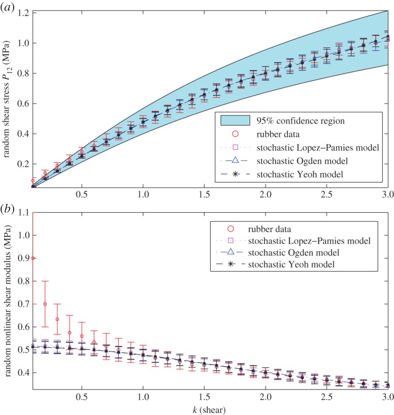
Calibrated stochastic models for rubber material subject to simple shear, with the parameters recorded in table 2, showing: (a) the random Piola–Kirchhoff shear stress P₁₂ (with the 95% confidence region for the Lopez–Pamies model, including the model mean values and standard deviations), and (b) the random nonlinear shear modulus $\hat{\mu }(k)$ of (2.12). (Online version in colour.)

(b). Brain mechanics

Example 5.2 mouse brainmouse brain —

In this example, we calibrate the random nonlinear shear modulus $\tilde{\mu }(a)$ of the stochastic one-term Ogden model (5.1) and of the stochastic multiple-term Ogden models of the form

$${\mathcal{W}}_n^{\mathrm{og}}=\sum _{p=1}^n[\frac{C_p}{2p^2}({\mathrm{\lambda }}_1^{2p}+{\mathrm{\lambda }}_2^{2p}+{\mathrm{\lambda }}_3^{2p}-3)+\frac{C_p}{2p^2}({\mathrm{\lambda }}_1^{-2p}+{\mathrm{\lambda }}_2^{-2p}+{\mathrm{\lambda }}_3^{-2p}-3)],$$ 5.4

with n=3,4,5, respectively, to mean values and standard deviation data for mouse brain tissue tested under 2% shear superposed on up to 40% tension or compression, in 10% increments. The nonlinear shear modulus of deterministic Ogden models with multiple terms was previously calibrated to similar mean values in [18]. Experimental tests on mouse brain tissue under small shear combined with axial deformations were reported on in [16]. The calibrated parameters and prior distribution hyperparameters of the stochastic models are recorded in table 3. For these models, the hyperparameters of the Gamma distribution for the random linear shear modulus $\overline{\mu }$ of (2.14) were obtained. Again, for multiple-term models, the choice of b is not unique. For a clear illustration, the random nonlinear shear modulus $\tilde{\mu }(a)$ of the one-term and four-term models are plotted in figure 2.

Then, for each model listed in table 3, we estimate the standard deviation that the mean shear modulus $\underset{\_}{\overline{\mu }}$ deviates from the mean data value D=0.1915 at 2% simple shear. Taking the models in the order of their complexity, from the simplest, one-term model, to the most complex, five-term model, we obtain:

$$\begin{array}{rl}\parallel D^{(1)}\parallel & =\frac{|0.2454-0.1915|}{2}=0.0270\text{for one-term (two-parameter) Ogden model},\\ \parallel D^{(2)}\parallel & =\frac{|0.2265-0.1915|}{2}=0.0175\text{for three-term (three-parameter) Ogden model},\\ \parallel D^{(3)}\parallel & =\frac{|0.2150-0.1915|}{2}=0.0117\text{for four-term (four-parameter) Ogden model},\\ \parallel D^{(4)}\parallel & =\frac{|0.2090-0.1915|}{2}=0.0087\text{for five-term (five-parameter) Ogden model}.\end{array}$$

When we compare each model to the next more complex one, by (4.4) and (4.5), the Bayes factors satisfy:

$$0.5143\le B_{12}\le 1.8806,0.5038\le B_{23}\le 1.9436,0.4983\le B_{34}\le \mathrm{1.9846.}$$

Assuming the prior odds of one model against another are all equal, the estimated bounds on the Bayes factors represent bounds on the posterior odds. From the above estimates, we first notice that the lower bounds appear to decrease, while the upper bounds tend to increase as the complexity of the models increases. However, as these changes are slow, we can only infer that the posterior odds for each model against another are approximately better than 1/2 (one to two) and worse than 2/1 (two to one), i.e. the posterior odds satisfy

$$\frac{1}{2}\le O_{ij}=\frac{P(D|M^{(i)})}{P(D|M^{(j)})}\le 2,i<j,\hspace{0.17em}i,j=1,2,3,4.$$

In this case, it is instructive to calculate also the approximate bounds on the corresponding posterior probabilities arising from these bounds. Taking P(D|M^(j))=1−P(D|M⁽ⁱ⁾), from the above double inequalities, we obtain 1/3≤P(D|M⁽ⁱ⁾)≤2/3, i=1,2,3,4. As these probabilities are close to 1/2, we conclude that the given data are equally probable according to the computations performed by the simplest or the more complicated models. Thus, given the accuracy of the approximations attained by different models, the explicit Bayesian approach cannot favour any particular model listed in table 3. Occam’s razor then implies that the simplest model should be chosen. In general, within a large set of possible models with no Bayesian favourite, it may not always be clear what ’the simplest model’ means. How do we quantify the notion of simplicity for different functions? However, in our case, we have a well-defined family of models with increasing number of terms. Therefore, we understand ’the simplest model’ as the one with the fewer number of terms, i.e. the one-term (two-parameter) stochastic Ogden model.

Table 3.

Calibrated parameters and prior distribution hyperparameters of stochastic Ogden-type models for mouse brain tissue, and the corresponding random linear shear modulus $\overline{\mu }$ of (2.14). The parameters are estimated by following the two-step strategy presented in §3.

stochastic model for mouse brain tissue	calibrated parameters (mean ± s.d.)	calibrated hyperparameters of prior probability distribution	random shear modulus (kPa) (mean ± s.d.)
one-term (two-parameter) Ogden (5.1)	c1=0.2454±0.0185	ρ1=175.6736	$\underset{\_}{\overline{\mu }}=0.2454\pm 0.0185$
	α1=−2.2111	ρ2=0.0014
three-term (three-parameter) Ogden (5.4)	c1=−1.1192±0.0255	ρ1=49.0153	$\underset{\_}{\overline{\mu }}=0.2265\pm 0.0324$
	c2=0.8167±0.0059	ρ2=0.0046
b=−3	c3=0.5291±0.0009	ξ1=7919
		ξ2=153 488
		ξ3=99 997
four-term (four-parameter) Ogden (5.4)	c1=−2.3043±0.3939	ρ1=57.7743	$\underset{\_}{\overline{\mu }}=0.2150\pm 0.0283$
	c2=1.7865±0.3491	ρ2=0.0037
b=−5	c3=1.1016±0.2035	ξ1=40
	c4=−0.3687±0.1305	ξ2=266
		ξ3=685
		ξ4=294
five-term (five-parameter) Ogden (5.4)	c1=−4.4681±0.0960	ρ1=51.4814	$\underset{\_}{\overline{\mu }}=0.2090\pm 0.0291$
	c2=2.5410±0.2452	ρ2=0.0041
b=−10	c3=3.4361±0.1178	ξ1=2771
	c4=−0.5959±0.0992	ξ2=2086
	c5=−0.7041±0.0969	ξ3=8388
		ξ4=6569
		ξ5=4502

Figure 2.

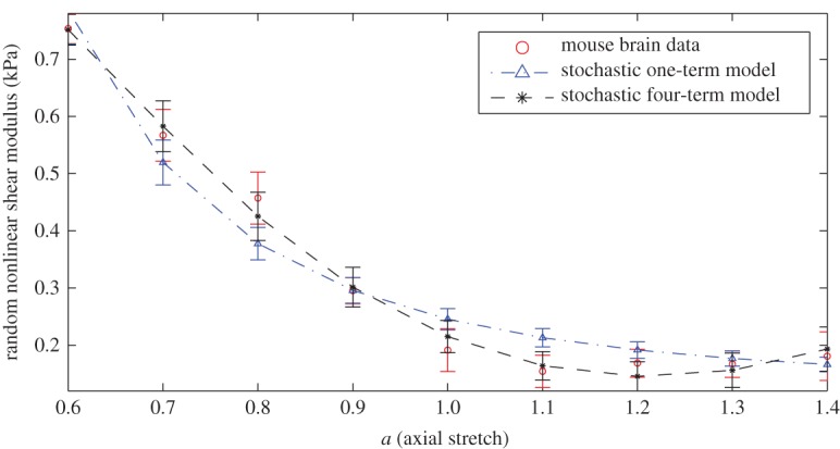
Calibrated stochastic Ogden models for mouse brain tissue under small shear superposed on finite axial stretch with the parameters listed in table 3, showing the random nonlinear shear modulus $\tilde{\mu }(a)$ of (2.13). (Online version in colour.)

Example 5.3 —

[human brain] Next, we calibrate the random nonlinear shear modulus $\tilde{\mu }(a)$ of the stochastic Ogden models (5.1) and (5.4), where n=3,4,5, to experimental data for human brain tissue under infinitesimal shear superposed on up to 25% tension or compression, in 5% increments. The nonlinear shear modulus of deterministic Ogden models with one or multiple terms was previously calibrated to the same mean values in [19]. Extensive experimental results for human brain tissue under combined shear and axial deformations were reported in [17], where the mean elastic responses were calculated as the average between the viscoelastic loading and unloading paths. The standard deviation considered here represents the range of viscoelastic responses. For the stochastic models, the calibrated parameters and prior distribution hyperparameters are given in table 4. For these models, the hyperparameters of the Gamma distribution for the random linear shear modulus $\overline{\mu }$ of (2.14) were identified. The random nonlinear shear modulus $\tilde{\mu }(a)$ of the one-term and four-term models are illustrated in figure 3.

As in the previous example, for each model recorded in table 4, we estimate the standard deviation that the mean linear shear modulus $\underset{\_}{\overline{\mu }}$ deviates from the known mean data value D=0.3379. We find:

$$\begin{array}{rl}\parallel D^{(1)}\parallel & =\frac{|0.3778-0.3379|}{2}=0.0200\text{for one-term (two-parameter) Ogden model},\\ \parallel D^{(2)}\parallel & =\frac{|0.3484-0.3379|}{2}=0.0053\text{for three-term (three-parameter) Ogden model},\\ \parallel D^{(3)}\parallel & =\frac{|0.3366-0.3379|}{2}=0.0006\text{for four-term (four-parameter) Ogden model},\\ \parallel D^{(4)}\parallel & =\frac{|0.3263-0.3379|}{2}=0.0058\text{for five-term (five-parameter) Ogden model}.\end{array}$$

By (4.4) and (4.5), the corresponding Bayes factors satisfy

$$0.4916\le B_{12}\le 1.9267,0.4830\le B_{23}\le 2.0336,0.4928\le B_{34}\le \mathrm{2.0702.}$$

Taking prior odds 1, the bounds on the Bayes factors represent bounds on posterior odds. Again, the above bounds are approximately at most 1/2 against the simpler model and at least 2/1 for the more complex one. Then, comparing one model with another, the posterior probability for each model satisfies 1/3<P(D|M⁽ⁱ⁾)<2/3, i=1,2,3,4, and is close to 1/2. Hence, by taking into account how well each model approximates the mean data, the explicit Bayesian approach does not favour any particular model listed in table 4. Applying Occam’s razor, the simplest model, i.e. the one-term (two-parameter) stochastic Ogden model, should be selected.

Table 4.

Calibrated parameters and prior distribution hyperparameters of stochastic Ogden-type models for human brain tissue, and the corresponding random linear shear modulus $\overline{\mu }$ of (2.14). The parameters are estimated by following the two-step strategy presented in §3.

stochastic model for human brain tissue	calibrated parameters (mean ± s.d.)	calibrated hyperparameters of prior probability distribution	random shear modulus (kPa) (mean ± s.d.)
one-term (two-parameter) Ogden (5.1)	c1=0.3778±0.0343	ρ1=121.3216	$\underset{\_}{\overline{\mu }}=0.3778\pm 0.0343$
	α1=−4.0250	ρ2=0.0031
three-term (three-parameter) Ogden (5.4)	c1=−5.5089±0.2859	ρ1=88.0208	$\underset{\_}{\overline{\mu }}=0.3484\pm 0.0371$
	c2=2.9269±0.2085	ρ2=0.0040
b=−10	c3=2.9305±0.1146	ξ1=203
		ξ2=2951
		ξ3=2074
four-term (four-parameter) Ogden (5.4)	c1=−13.5515±0.3164	ρ1=82.3576	$\underset{\_}{\overline{\mu }}=0.3366\pm 0.0371$
	c2=10.3735±0.2367	ρ2=0.0041
b=−15	c3=6.8913±0.1296	ξ1=20
	c4=−3.3767±0.0128	ξ2=7643
		ξ3=22 661
		ξ4=7236
five-term (five-parameter) Ogden (5.4)	c1=−35.9407±0.9719	ρ1=74.9717	$\underset{\_}{\overline{\mu }}=0.3263\pm 0.0377$
	c2=20.2082±0.3292	ρ2=0.0044
b=−50	c3=29.9337±1.1963	ξ1=198
	c4=−6.9335±0.1919	ξ2=30 726
	c5=−6.9413±0.3994	ξ3=2979
		ξ4=44 696
		ξ5=16 329

Figure 3.

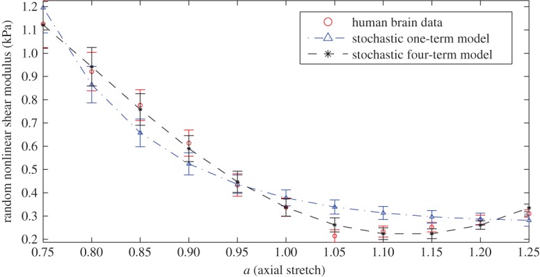
Calibrated stochastic Ogden-type models for human brain tissue under small shear superposed on finite axial stretch, with the parameters given in table 4, showing the random nonlinear shear modulus $\tilde{\mu }(a)$ of (2.13). (Online version in colour.)

Remark 5.4 —

It is important to remark here that the estimated bounds on the Bayes factors in the two examples involving brain tissue data [18,19] are very similar. Further numerical tests that are not included here also show that similar bounds, i.e. approximately 1/2 and 2, respectively, are found when simple shear superposed on the maximum compression or tension is considered, or when models with more terms are calibrated to the given datasets. By the likelihood principle, we infer that the two datasets have the same likelihood [76]. This is very striking, given that the respective data arise from different brain tissue types tested by different experimental procedures. In this case, the likelihood principle seems to play a unifying role for the experimental testing. A natural question is then: could this principle be further applied to guide experiments?

6. Conclusion

Homogeneous isotropic hyperelastic models can capture characteristic mechanical behaviours of many deformable solids and underpin their analyses and computer simulation. However, natural and bioinspired materials exhibit inherent variations in their elastic properties, which play important roles in their functional performance, and are not represented by a nonlinear elastic constitutive law. For these materials, stochastic representations accounting also for data dispersion contain additional information about the variability of material properties. We combine finite elasticity and information theories to construct homogeneous isotropic hyperelastic models with random field parameters calibrated to discrete mean values and standard deviations of either the stress–strain function or the nonlinear shear modulus, which is a function of the deformation, estimated from experimental tests. These quantities can take on different values, corresponding to possible outcomes of the experiments. In summary, we cast the model parameters as random variables and use the maximum entropy probability distribution to express the uncertainty of the data variability. In our approach, the mean values and standard deviations of the model parameters and the hyperparameters of the underlying probability distribution are calculated formally, although these quantities are not unique in general. As multiple models, which differ in form or number of parameters, can be derived that adequately represent the observed phenomena, we apply Occam’s razor by providing an explicit criterion for model selection, based on Bayesian statistics. We then employ this criterion to select a model among competing models calibrated to the available data for rubber and brain tissues under single or multiaxial loads. Our modelling strategy can further be used to study the variation in the elastic behaviour of solid materials in different applications. In medicine, this research enhances the current solid mechanics research as it will enable better predictions from ensemble data.

Data accessibility

The datasets for this article have been uploaded as supplementary material.

Authors' contributions

All authors contributed equally to all aspects of this article and gave their final approval for publication.

Competing interests

We declare we have no competing interests.

Funding

The support for L.A.M. by the Engineering and Physical Sciences Research Council of Great Britain under research grant no. EP/M011992/1 is gratefully acknowledged.

References

- 1.McCoy JJ. 1973. A statistical theory for predicting response of materials that possess a disordered structure. Technical Report ARPA 2181, AMCMS Code 5911.21.66022. Watertown, MA: Army Materials and Mechanics Research Center.
- 2.Huet C. 1990. Application of variational concepts to size effects in elastic heterogeneous bodies. J. Mech. Phys. Solids 38, 813–841. (doi:10.1016/0022-5096(90)90041-2) [Google Scholar]
- 3.Ostoja-Starzewski M. 2008. Microstructural randomness and scaling in mechanics of materials. New York, NY: Chapman and Hall/CRC. [Google Scholar]
- 4.Hauseux P, Hale JS, Bordas SPS. 2017. Accelerating Monte Carlo estimation with derivatives of high-level finite element models. Comput. Methods Appl. Mech. Eng. 318, 917–936. (doi:10.1016/j.cma.2017.01.041) [Google Scholar]
- 5.Madireddy S, Sista B, Vemaganti K. 2015. A Bayesian approach to selecting hyperelastic constitutive models of soft tissue. Comput. Methods Appl. Mech. Eng. 291, 102–122. (doi:10.1016/j.cma.2015.03.012) [Google Scholar]
- 6.Madireddy S, Sista B, Vemaganti K. 2016. Bayesian calibration of hyperelastic constitutive models of soft tissue. J. Mech. Behav. Biomed. Mater. 59, 108–127. (doi:10.1016/j.jmbbm.2015.10.025) [DOI] [PubMed] [Google Scholar]
- 7.Babuška I, Nobile F, Tempone R. 2007. Reliability of computational science. Numer. Methods Partial.Differ. Equ. 23, 753–784. (doi:10.1002/num.20263) [Google Scholar]
- 8.Babuška I, Nobile F, Tempone R. 2008. A systematic approach to model validation based on Bayesian updates and prediction related rejection criteria. Comput. Methods Appl. Mech. Eng. 197, 2517–2539. (doi:10.1016/j.cma.2007.08.031) [Google Scholar]
- 9.Oden JT, Moser R, Ghattas O. 2010. Computer predictions with quantified uncertainty, part I. SIAM News 43, 1–3. [Google Scholar]
- 10.Oden JT, Moser R, Ghattas O. 2010. Computer predictions with quantified uncertainty, part II. SIAM News 43, 1–4. [Google Scholar]
- 11.Oden JT, Prudencio EE, Hawkins-Daarud A. 2013. Selection and assessment of phenomenological models of tumor growth. Math. Models Methods Appl. Sci. 23, 1309–1338. (doi:10.1142/S0218202513500103) [Google Scholar]
- 12.Farmer CL. 2017. Uncertainty quantification and optimal decisions. Proc. R. Soc. A 473, 20170115 (doi:10.1098/rspa.2017.0115) [DOI] [PMC free article] [PubMed] [Google Scholar]
- 13.dell’Isola F, Giorgio I, Pawlikowski M, Rizzi NL. 2016. Large deformations of planar extensible beams and pantographic lattices: heuristic homogenization, experimental and numerical examples of equilibrium. Proc. R. Soc. A 472, 20150790 (doi:10.1098/rspa.2015.0790) [Google Scholar]
- 14.Placidi L, Barchiesi E, Turco E, Rizzi NL. 2016. A review on 2D models for the description of pantographic fabrics. Zeitschrift für angewandte Mathematik und Physik 67, 121 (doi:10.1007/s00033-016-0716-1) [Google Scholar]
- 15.Perepelyuk M, Chin LK, Cao X, van Oosten A, Shenoy VB, Janmey PA, Wells RG. 2016. Normal and fibrotic rat livers demonstrate shear strain softening and compression stiffening: a model for soft tissue mechanics. PLoS ONE 11, e0146588 (doi:10.1371/journal.pone.0146588) [DOI] [PMC free article] [PubMed] [Google Scholar]
- 16.Pogoda K. et al. 2014. Compression stiffening of brain and its effect on mechanosensing by glioma cells. New J. Phys. 16, 075002 (doi:10.1088/1367-2630/16/7/075002) [DOI] [PMC free article] [PubMed] [Google Scholar]
- 17.Budday S. et al. 2017. Mechanical characterization of human brain tissue. Acta Biomater. 48, 319–340. (doi:10.1016/j.actbio.2016.10.036) [DOI] [PubMed] [Google Scholar]
- 18.Mihai LA, Chin L, Janmey PA, Goriely A. 2015. A comparison of hyperelastic constitutive models applicable to brain and fat tissues. J. R. Soc. Interface 12, 20150486 (doi:10.1098/rsif.2015.0486) [DOI] [PMC free article] [PubMed] [Google Scholar]
- 19.Mihai LA, Budday S, Holzapfel GA, Kuhl E, Goriely A. 2017. A family of hyperelastic models for human brain tissue. J. Mech. Phys. Solids 106, 60–79. (doi:10.1016/j.jmps.2017.05.015) [Google Scholar]
- 20.Kloczkowski A. 2002. Application of statistical mechanics to the analysis of various physical properties of elastomeric networks–a review. Polymer 43, 1503–1525. (doi:10.1016/S0032-3861(01)00588-2) [Google Scholar]
- 21.Chagnon G, Rebouah M, Favier D. 2014. Hyperelastic energy densities for soft biological tissues: a review. J. Elast. 120, 129–160. (doi:10.1007/s10659-014-9508-z) [Google Scholar]
- 22.Fu YB, Chui CK, Teo CL. 2013. Liver tissue characterization from uniaxial stress-strain data using probabilistic and inverse finite element methods. J. Mech. Behav. Biomed. Mater. 20, 105–112. (doi:10.1016/j.jmbbm.2013.01.008) [DOI] [PubMed] [Google Scholar]
- 23.Staber B, Guilleminot J. 2015. Stochastic modeling of a class of stored energy functions for incompressible hyperelastic materials with uncertainties. C R Mécanique 343, 503–514. (doi:10.1016/j.crme.2015.07.008) [Google Scholar]
- 24.Staber B, Guilleminot J. 2016. Stochastic modeling of the Ogden class of stored energy functions for hyperelastic materials: the compressible case. J. Appl. Math. Mech. 97, 273–295. (doi:10.1002/zamm.201500255) [Google Scholar]
- 25.Staber B, Guilleminot J. 2017. Stochastic hyperelastic constitutive laws and identification procedure for soft biological tissues with intrinsic variability. J. Mech. Behav. Biomed. Mater. 65, 743–752. (doi:10.1016/j.jmbbm.2016.09.022) [DOI] [PubMed] [Google Scholar]
- 26.Guilleminot J, Soize C. 2012. Generalized stochastic approach for constitutive equation in linear elasticity: a random matrix model. Int. J. Numer. Methods Eng. 90, 613–635. (doi:10.1002/nme.3338) [Google Scholar]
- 27.Guilleminot J, Soize C. 2013. On the statistical dependence for the components of random elasticity tensors exhibiting material symmetry properties. J. Elast. 11, 109–130. [Google Scholar]
- 28.Jaynes ET. 1957. Information theory and statistical mechanics I. Phys. Rev. 108, 171–190. (doi:10.1103/PhysRev.108.171) [Google Scholar]
- 29.Jaynes ET. 1957. Information theory and statistical mechanics II. Phys. Rev. 106, 620–630. (doi:10.1103/PhysRev.106.620) [Google Scholar]
- 30.Jaynes ET. 2003. Probability theory: the logic of science. Cambridge, UK: Cambridge University Press. [Google Scholar]
- 31.Shannon CE. 1948. A mathematical theory of communication. Bell System Tech. J. 27, 379–423, 623–659 (doi:10.1002/j.1538-7305.1948.tb01338.x) [Google Scholar]
- 32.Soni J, Goodman R. 2017. A mind at play: how Claude Shannon invented the information age. New York, NY: Simon & Schuster. [Google Scholar]
- 33.Truesdell C, Noll W. 2004. The non-linear field theories of mechanics, 3rd edn New York, NY: Springer. [Google Scholar]
- 34.Ogden RW. 1997. Non-linear elastic deformations, 2nd edn New York, NY: Dover. [Google Scholar]
- 35.Goriely A. 2017. The mathematics and mechanics of biological growth. New York, NY: Springer. [Google Scholar]
- 36.Holzapfel GA. 2000. Nonlinear solid mechanics: a continuum approach for engineering. New York, NY: John Wiley & Sons. [Google Scholar]
- 37.Hadamard J. 1902. Sur les problémes aux dérivées partielles et leur signification physique. Princeton University Bulletin, pp. 49–52.
- 38.Ball JM. 1977. Convexity conditions and existence theorems in non-linear elasticity. Arch. Ration. Mech. Anal. 63, 337–403. (doi:10.1007/BF00279992) [Google Scholar]
- 39.Balzani D, Neff P, Schröder J, Holzapfel GA. 2006. A polyconvex framework for soft biological tissues. Adjustment to experimental data. Int. J. Solids Struct. 43, 6052–6070. (doi:10.1016/j.ijsolstr.2005.07.048) [Google Scholar]
- 40.Abramowitz M, Stegun IA. 1964. Handbook of mathematical functions with formulas, graphs, and mathematical tables, Applied Mathematics Series, vol. 55, Washington, DC: National Bureau of Standards.
- 41.Johnson NL, Kotz S, Balakrishnan N. 1994. Continuous univariate distributions, vol. 1, 2nd edn New York, NY: John Wiley & Sons. [Google Scholar]
- 42.Mihai LA, Goriely A. 2017. How to characterize a nonlinear elastic material? A review on nonlinear constitutive parameters in isotropic finite elasticity. Proc. R. Soc. A 473, 20170607 (doi:10.1098/rspa.2017.0607) [DOI] [PMC free article] [PubMed] [Google Scholar]
- 43.Baker M, Ericksen JL. 1954. Inequalities restricting the form of the stress-deformation relations for isotropic elastic solids and Reiner-Rivlin fluids. J. Wash. Acad. Sci. 44, 24–27. [Google Scholar]
- 44.Marzano M. 1983. An interpretation of Baker-Ericksen inequalities in uniaxial deformation and stress. Meccanica 18, 233–235. (doi:10.1007/BF02128248) [Google Scholar]
- 45.Destrade M, Saccomandi G, Sgura I. 2017. Methodical fitting for mathematical models of rubber-like materials. Proc. R. Soc. A 473, 20160811 (doi:10.1098/rspa.2016.0811) [Google Scholar]
- 46.Mihai LA, Neff P. 2017. Hyperelastic bodies under homogeneous Cauchy stress induced by non-homogeneous finite deformations. Int. J. Nonlinear Mech. 89, 93–100. (doi:10.1016/j.ijnonlinmec.2016.12.003) [Google Scholar]
- 47.Mihai LA, Neff P. 2017. Hyperelastic bodies under homogeneous Cauchy stress induced by three-dimensional non-homogeneous deformations. Math. Mech. Solids (doi:10.1177/1081286516682556) [Google Scholar]
- 48.Neff P, Mihai LA. 2016. Injectivity of the Cauchy-stress tensor along rank-one connected lines under strict rank-one convexity condition. J. Elast. 127, 309–315. (doi:10.1007/s10659-016-9609-y) [Google Scholar]
- 49.Truesdell C. 1956. Das ungelöste Hauptproblem der endlichen Elastizitätstheorie. J. Appl. Math. Mech. 36, 97–103. (doi:10.1002/zamm.19560360304) [Google Scholar]
- 50.Ball JM, James RD. 2002. The scientific life and influence of Clifford Ambrose Truesdell III. Arch. Ration. Mech. Anal. 161, 1–26. (doi:10.1007/s002050100178) [Google Scholar]
- 51.Ball JM. 2002. Some open problems in elasticity. In Geometry, mechanics, and dynamics (eds P Newton, P Holmes, A Weinstein), pp. 3–59. New York, NY: Springer.
- 52.Bayes T. 1763. An essay toward solving a problem in the doctrine of chances. Phil. Trans. R. Soc. Lond. 53, 370–418. (doi:10.1098/rstl.1763.0053) [PubMed] [Google Scholar]
- 53.Thorburn WM. 1918. The myth of Occam’s razor. Mind 27, 345–353. (doi:10.1093/mind/XXVII.3.345) [Google Scholar]
- 54.Jefferys WH, Berger JO. 1992. Ockham’s razor and Bayesian analysis. Am. Sci. 80, 64–72. [Google Scholar]
- 55.Jeffreys H. 1935. Some tests of significance, treated by the theory of probability. Math. Proc. Camb. Philos. Soc. 31, 203–222. (doi:10.1017/S030500410001330X) [Google Scholar]
- 56.Jeffreys H. 1961. Theory of probability, 3rd edn Oxford, UK: Oxford University Press. [Google Scholar]
- 57.Berger JO, Jefferys WH. 1992. The application of robust Bayesian analysis to hypothesis testing and Occam’s razor. J. Italian Stat. Soc. 1, 17–32. (doi:10.1007/BF02589047) [Google Scholar]
- 58.Rajagopal KR, Wineman AS. 1987. New universal relations for nonlinear isotropic elastic materials. J. Elast. 17, 75–83. (doi:10.1007/BF00042450) [Google Scholar]
- 59.Destrade M, Murphy JG, Saccomandi G. 2012. Simple shear is not so simple. Int. J. Nonlinear Mech. 47, 210–214. (doi:10.1016/j.ijnonlinmec.2011.05.008) [Google Scholar]
- 60.Mihai LA, Goriely A. 2011. Positive or negative Poynting effect? The role of adscititious inequalities in hyperelastic materials. Proc. R. Soc. A 467, 3633–3646. (doi:10.1098/rspa.2011.0281) [Google Scholar]
- 61.Mihai LA, Goriely A. 2013. Numerical simulation of shear and the Poynting effects by the finite element method: an application of the generalised empirical inequalities in non-linear elasticity. Int. J. Nonlinear Mech. 49, 1–14. (doi:10.1016/j.ijnonlinmec.2012.09.001) [Google Scholar]
- 62.Ericksen JL. 1954. Deformations possible in every isotropic, incompressible, perfectly elastic body. Z. Angew. Math. Phys. 5, 466–489. (doi:10.1007/BF01601214) [Google Scholar]
- 63.Ericksen JL. 1955. Deformation possible in every compressible isotropic perfectly elastic materials. J. Math. Phys. 34, 126–128. (doi:10.1002/sapm1955341126) [Google Scholar]
- 64.Shield RT. 1971. Deformations possible in every compressible, isotropic, perfectly elastic material. J. Elast. 1, 91–92. (doi:10.1007/BF00045703) [Google Scholar]
- 65.Singh M, Pipkin AC. 1965. Note on Ericksen’s problem. Z. Angew. Math. Phys. 16, 706–709. (doi:10.1007/BF01590971) [Google Scholar]
- 66.Ogden RW. 1972. Large deformation isotropic elasticity–on the correlation of theory and experiment for incompressible rubberlike solids. Proc. R. Soc. A 326, 565–584. (doi:10.1098/rspa.1972.0026) [Google Scholar]
- 67.Lopez-Pamies O. 2010. A new I1-based hyperelastic model for rubber elastic materials. C R Mécanique 338, 3–11. (doi:10.1016/j.crme.2009.12.007) [Google Scholar]
- 68.Arruda EM, Boyce MC. 1993. A three-dimensional constitutive model for the large stretch behavior of rubber elastic materials. J. Mech. Phys. Solids 41, 389–412. (doi:10.1016/0022-5096(93)90013-6) [Google Scholar]
- 69.Yeoh OH. 1990. Characterization of elastic properties of carbon-black-filled rubber vulcanizates. Rubber Chem. Technol. 63, 792–805. (doi:10.5254/1.3538289) [Google Scholar]
- 70.Yeoh OH. 1993. Some forms of the strain energy function for rubber. Rubber Chem. Technol. 66, 754–771. (doi:10.5254/1.3538343) [Google Scholar]
- 71.Ogden RW, Saccomandi G, Sgura I. 2004. Fitting hyperelastic models to experimental data. Comput. Mech. 34, 484–502. (doi:10.1007/s00466-004-0593-y) [Google Scholar]
- 72.Soize C. 2000. A nonparametric model of random uncertainties for reduced matrix models in structural dynamics. Probabilis. Eng. Mech. 15, 277–294. (doi:10.1016/S0266-8920(99)00028-4) [Google Scholar]
- 73.Soize C. 2001. Maximum entropy approach for modeling random uncertainties in transient elastodynamics. J. Acoust. Soc. Am. 109, 1979–1996. (doi:10.1121/1.1360716) [DOI] [PubMed] [Google Scholar]
- 74.Kotz S, Balakrishnan N, Johnson NL. 2000. Continuous multivariate distributions vol. 1: models and applications, 2nd edn. New York, NY: Wiley. [Google Scholar]
- 75.Nunes ICS, Moreira DC. 2013. Simple shear under large deformation: experimental and theoretical analyses. Eur. J. Mech. A, Solids 42, 315–322. (doi:10.1016/j.euromechsol.2013.07.002) [Google Scholar]
- 76.Edwards W, Lindman H, Savage LJ. 1863. Bayesian statistical inference for physiological research. Psychol. Rev. 70, 193–242. (doi:10.1037/h0044139) [Google Scholar]
Associated Data
This section collects any data citations, data availability statements, or supplementary materials included in this article.
Supplementary Materials
Data Availability Statement