Open-path dual comb spectroscopy to an airborne retroreflector

Abstract

We demonstrate a new technique for spatial mapping of multiple atmospheric gas species. This system is based on high-precision dual-comb spectroscopy to a retroreflector mounted on a flying multi-copter. We measure the atmospheric absorption over long open-air paths to the multi-copter with comb-tooth resolution over 1.57 to 1.66 pm, covering absorption bands of CO₂, Cm, H₂O and isotopologues. When combined with GPS-based path length measurements, a fit of the absorption spectra retrieves the dry mixing ratios versus position. Under well-mixed atmospheric conditions, retrievals from both horizontal and vertical paths show stable mixing ratios as expected. This approach can support future boundary layer studies as well as plume detection and source location.

Open-path dual frequency comb spectroscopy (DCS) has recently been shown to provide highly accurate and resolved broadband atmospheric spectra across kilometer-scale paths to fixed reflectors [1–3]. This makes DCS well suited to measurements and quantification of emissions of pollutants, hazardous gases, and greenhouse gases. In a recent direct intercomparison, two open-path DCS retrieved atmospheric traces gas mixing ratios to within 0.14% – 0.4% over weeks, well below the natural atmospheric variability [3]. Here we describe an advance in open-path DCS that enables measurements of the horizontal and vertical spatial profile of atmospheric gases in near real time. This technique, especially when extended to other spectral regions, has a variety of potential applications such as emissions quantification, boundary-layer profiling, and hazardous plume detection. For example, emissions from oil and gas facilities are important both for understanding global methane sources [4–6] and for understanding the impacts on ozone and aerosol formation [7–9]. By flying box type patterns around a distributed source and using a mass-balance approach [10,11], such a system could be used to quantify CH₄ as well as volatile organic compounds. In addition, the mixing of gases within the planetary boundary layer is currently a major source of uncertainty in atmospheric transport models [12–14], which results in errors in source quantification using point sensors or satellites. Finally, this technique could be used to rapidly scan an area for the presence of hazardous gases [15] and threat chemicals [16].

Unlike differential absorption LIDAR [17,18], which measures the atmospheric absorption at only a few laser frequencies, DCS measures the spectrum at many tens of thousands of individual frequencies with eye-safe near-infrared (or, in the future mid-infrared) laser light [19,20]. As a consequence of this massively broadband nature, open-path DCS requires a reflector at the far end of the path to provide sufficient signal-to-noise ratio. Here, we demonstrate DCS to a retroreflector that is mounted on a multi-copter, part of a small unmanned aircraft system (sUAS), as illustrated in Figure 1. This combined sUAS-DCS system is used to scan horizontal and vertical paths and retrieve the column-integrated mixing ratios of water, CO₂, and CH₄. With future extensions across even broader near-infrared bandwidths and into the mid-infrared, such a system could provide spatial mapping across multiple gas species at high precision and accuracy.

Figure 1.

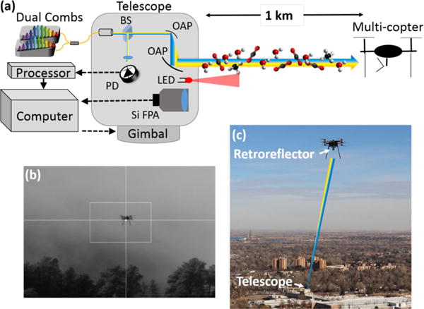
Setup for DCS to a sUAS. (a) The light from both combs is combined in fiber, then launched from a telescope to a retroreflector on a small multicopter. A co-aligned 850-nm LED and silicon focal plane array (Si FPA) camera are used in the tracking servo to control the azimuth-elevation gimbal. PD: photodetector: BS: beam splitter: OAP: off-axis parabolic mirror (b) Image from Si FPA showing the multi-copter above the tree line. The bright spot is the retroreflected 850 nm LED light. A software feedback loop to the telescope gimbal centers this spot on the cross hairs, which simultaneously maximizes the DCS signal on the photodetector, (c) Photo of the small commercial multi-copter. The dual-comb light is launched from the telescope located in the 1-km distant rooftop laboratory, as indicated.

The DCS system is described in detail in Ref. [21]. It is based on two near-infrared, self-referenced, optically coherent fiber frequency combs [22] with repetition rates of f_r ~ 200 MHz that differ by Δf_rep = 624 Hz. A portion of each frequency comb is amplified, spectrally broadened in highly nonlinear fiber, combined in fiber, and filtered to cover 1.57–1.66 pm (or 6000 cm⁻¹ to 6330 cm⁻¹) which allows simultaneous measurements of CO₂, CH₄, H₂O and isotopologues. The mutual comb linewidth was below 1 Hz and the absolute long-term linewidth was below 120 kHz, enabling ultra-high resolution sampling of the atmospheric spectrum at f_r ~200 MHz point spacing over ~50,000 comb teeth. The entire system is compact and portable [21], and has been operated in non-laboratory environments [3,23].

The telescope system, sketched in Fig. 1a, was designed for a large collection aperture while remaining relatively lightweight and compact for rapid scanning. About 5 mW of the filtered light is sent to the launch telescope system for the open-path measurements. This launched power is below 9.6 mW at the telescope aperture, which is the Class 1 ANSI accessible emission limit (AEL) [24]. Only reflective optics were used to enable broad spectral bandwidth operation. The telescope uses two off-axis parabolic mirrors with a 3″-diameter collection aperture, resulting in a launched beam diameter of ~45 mm with a nearly diffraction-limited beam divergence of ~30 prad (half-angle). This telescope was mounted on a gimbal to allow pointing and tracking to the retroreflector. The gimbal was capable of both elevation and azimuthal motion with a velocity of 80 deg/s and an acceleration of400 deg/s².

The multi-copter (xFold Cinema x8 [25]) with payload is shown flying in Figs. 1b and 1c. The primary payload is a commercially available, light-weight, 2.5″-diameter, 5-arcsecond angular-deviation hollow corner-cube retroreflector. The use of a corner-cube retroreflector on the multi-copter, rather than a plane mirror, drastically reduces the multi-copter pointing requirements. Since the retroreflector has a wide field-of-view (approximately ±15°), we can rely solely on yaw control of the multi-copter to maintain sufficient pointing back to the telescope. The payload included a radiosonde (i-Met RSB 1 [25]) for temperature, pressure, relative humidity, and realtime coarse GPS location. Finally, the payload also included a real-time kinematic GPS (RTK GPS, Swift Navigation Piksi [25]) for high-precision differential path length measurements.

The precision of the mixing ratios retrieved by the DCS depends on both received power and averaging time. Received powers range from a minimum of ~ 15 μW up to typical levels of a few hundred microwatts, above which the detector saturates. At typical average received power levels of ~50–100 pW, the measurement precision in ~10 seconds was 2 ppm of CO₂ and 16 ppb CH₄ and improved to 0.6 ppm of CO₂ and 6 ppb of CH4 in ~100 s (see [3] for a full Allan deviation. To support these averaging times, we used a “step scan” approach: the sUAS moves the retroreflector to a specific location where it hovers for a user-selected time before moving to a new location. The total flight time for a single battery charge was ~15 minutes under our flight conditions.

The telescope system must track the motion of the retroreflector as it moves and hovers in order to obtain sufficient return power of the DCS comb light. Ideally, this tracking is within the ~30-prad beam divergence but this requirement is reduced (at the cost of reduced return power by about a factor of two because of turbulence-induced fast angular jitter [26]. The telescope tracking was based on feedback from a focal plane array (FPA) that imaged the return from the retroreflector. Direct use of the near-infrared DCS light would require an expensive InGaAs camera and would not provide a large angular capture range. To circumvent these limitations, we launch a high-power, low-divergence 850 nm LED co-aligned with the DCS light. At this wavelength, the reflected LED light can be detected by a silicon FPA. The return LED light is bandpass filtered and imaged onto this FPA with a 500-mm-focal-length, 85-mm-diameter camera lens (typical image shown in Fig. 1b). The images are read out at 30-Hz into a computer, averaged over two frames, smoothed by a 3-pixel Gaussian filter, and then processed to find the retroreflector location via two-dimensional peak finding. The offset of the identified intensity maximum from the target location (shown as cross hairs in Fig. 1b) was input to a proportional plus double-integral loop whose output controlled the telescope pointing at 15 Hz with a ~2 Hz integration bandwidth, which was sufficient for these measurements. In the future, the feedback bandwidth could be improved by a higher frame rate camera and the tracking during movement could be improved with more sophisticated estimation algorithms (such as a Kalman filter). The retro-reflected dual comb light is collected by the off-axis telescope and focused onto a ~100-MHz-bandwidth amplified InGaAs photodetector using a non-polarizing beamsplitter, as shown in Fig. 1a. The total loss of the telescope system (collected return power compared to input power to the telescope) was typically ~8–20 dB depending on atmospheric conditions (e.g. turbulence-induced scintillation or wind gusts impacting sUAS yaw stability). We achieved ~ 5 dB higher overall collected light by use of a polarizing beamsplitter and quarter-wave plate to act as an optical circulator; however, this created additional etalons which negated the benefits of higher power.

For the analysis, we need the path length, air temperature, and air pressure. The path length is determined using either the radiosonde GPS and known GPS location of the telescope system, or preferably with the RTK GPS, which measures the differential path length between a receiver on the sUAS and a receiver located near the telescope system. The RTK-GPS provides the path length to < 6 cm accuracy at 10-Hz sampling rate, but requires signals from at least 7 GPS satellites and was available for only one of the two flight tests described below. We used an average temperature determined from the radiosonde on the sUAS and a sensor located near the telescope. The pressure is taken from the radiosonde.

The DCS signal is a series of interferograms that repeat at a rate of Δf_rep = 624 Hz, or once every 1.6 ms. We coherently sum 100 of these interferograms on a field-programmable gate array, and then further carrier-phase correct and sum N sets in software, yielding one interferogram (and thus spectrum) every 100 N/Δf_rep seconds (here N ranged from 60–200, resulting in one spectrum every10–30 s). Each spectrum is fit to an absorption model based on HITRAN 2008 [27] plus a piecewise-polynomial baseline to account for the comb spectral structure, as discussed in [3].

We flew two different flight patterns on December 1, 2016. The first flight pattern, shown by the yellow track in Fig. 2a, consisted primarily of horizontal movement with respect to the telescope. Near real-time results are shown as a movie in Visualization 1. In Visualization 1, the lower right quadrant shows the real-time updates of the measured atmospheric spectrum and the lower left quadrant shows the real-time mixing ratios retrieved under a simplified assumption of a fixed 2-km path length, fixed temperature, and fixed pressure. In post processing, we re-fit the raw spectra with the measured time-dependent path length, temperature, and pressure. Figure 2b shows the retrieved path-length-corrected mixing ratios as a function of time at 9.6-s averaging times along with the multi-copter location, and radiosonde GPS-measured path length. Prior to 13:07 local time the multi-copter was stationary on a platform. After take-off at ~13:07, it hovered for 1–3 minutes at five different locations, as indicated in the position graphs. During transit, the return power fluctuated, but it was generally well above the 15-μW minimum threshold during hovering. From 13:16 to 13:17, the sUAS did not maintain sufficient multi-copter yaw to point the retroreflector back to the telescope and signal was lost. Signal was regained at ~ 13:17, but subsequent loss of sUAS telemetry caused the multi-copter to then return to the platform. The mixing ratios are fairly constant over the flight pattern as expected over this ~100×60 m² area and prevailing ~1 m/s wind speed.

Figure 2.

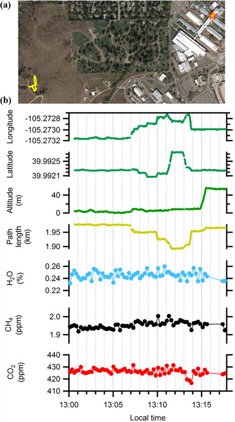
(a) Flight path (yellow) recorded by the radiosonde GPS for the first flight pattern. The orange star indicates the DCS and telescope location. Map data: Google, DigitalGlobe, U.S. Geological Survey, USDA Farm Service Agency. A video ofthe real-time data collection software for this flight is given in Visualization 1. (b) Mixing ratios for H₂O (blue), CH₄ (black), and CO₂ (red) obtained from the horizontal flight path shown in Fig. 2b. These data are from spectra acquired every 9.6 seconds and are corrected for measured path length, temperature and pressure. The upper four panels show the latitude, longitude, altitude, and path length derived from the radiosonde GPS.

The second flight pattern consisted of a series of slant-column measurements - as illustrated in Fig. 3 – from near ground level up to the 120-meter (400-foot) ceiling height imposed by current Federal Aviation Agency (FAA) regulations [28]. Higher flights are possible with FAA approval and will be pursued in the future to study boundary layer variations of the trace gas concentrations. As with the horizontal path measurements, a move-hover pattern was used; the multi-copter was flown to a specific altitude, where it hovered for ~4 minutes before ascending/descending to another altitude. From 14:33 to 14:36, the multi-copter returned to the platform to exchange batteries. The overall flight duration was ~25 minutes. The RTK-GPS was operational during the full flight. In addition, a fixed horizontal path was acquired simultaneously using a second output from the same DCS instrument directed by a second telescope to a fixed retroreflector located near the launch point of the multi-copter.

Figure 3.

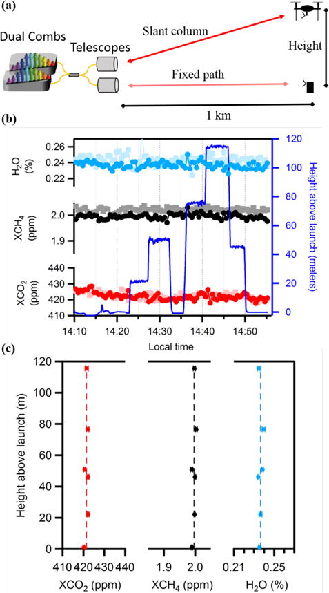
Results of a flight to obtain a vertical concentration profile. (a) Diagram showing simultaneous slant column and fixed path measurements. (b) The path-corrected H₂O (medium blue), dry CH₄ (black), and dry CO₂ (red) mixing ratios obtained for 32-s averaged data from the sUAS-DCS. The data in lighter colors were obtained along the fixed path. The corresponding retroreflector height above ground (from the RTK GPS) is also shown (right axis, dark blue). (c) Slant-column mixing ratio versus altitude from averaging approximately ten points over 4–5 minutes at each height in (b). The error bars are the standard error of the mean. Averaged over height (dashed line), the mixing ratios are 421.5 ± 0.9 ppm, 1.996 ± 0.006 ppm, and 0.236 ± 0.002 % for CO₂, CH₄, and H₂O, respectively. The scatter about the mean is attributed to temporal, rather than spatial, variations under these well-mixed conditions.

The fitted mixing ratios for both paths as well as corresponding sUAS height from the RTK GPS are shown in Fig. 3b. These data were acquired at wind speeds of ~0.5–5 m/s and with a forecast boundary layer height of ~2 km [29]; therefore, we also expect strong mixing of the atmosphere over the measured altitudes and relatively constant mixing ratios. We can determine the variation in slant column versus height by averaging all measurements at a given height bin, as is shown in Fig. 3c. The residual scatter of these binned data is ~0.87 ppmv CO₂, 5.7 ppbv CH₄, and 0.0021 % H₂O. As expected from the atmospheric conditions, there is no clear structure versus height. This lack of variability contrasts with the measurements of Ref. [3], acquired over longer timescale and sometimes at lower wind speed, where significant temporal variations are observed both on diurnal timescales and shorter timescales as plumes traverse the open-path beam. We do observe some temporal variability here, as seen for example in the ~ 5 ppm decrease in XCO₂ over the measurement time in Fig. 3b. However, this same XCO₂ decrease is observed simultaneously on the slant paths and fixed horizontal path, indicating it reflects a temporal rather than vertical variability, again reflecting the well-mixed conditions. (The ~25 ppb constant offset in CH₄ between the horizontal and slant path measurements is attributed to nonlinearities when combining the two combs in fiber and have been resolved [3]. In contrast, in less-well-mixed conditions or if the retroreflector height had exceeded the boundary layer, one would expect stronger variations. For example, photosynthesis can cause CO₂ gradients in the boundary layer of 1–10 ppm [30]. In regions with higher emissions, the variations in CO₂ or CH₄ between the boundary layer and free troposphere could be 20 ppm or more for CO₂ [31] and 100 ppb or more for CH₄ [32]. These changes are easily within our precision of <1 ppm for CO₂ and <6 ppb for CH₄; we intend to explore such vertical structures in future campaigns.

Here, we demonstrated simultaneous detection of CO₂, CH₄, and H₂O along a 2-km-roundtrip path using dual comb spectroscopy with a retroreflector located on a sUAS. In the future, additional species could be detected with broader wavelength coverage and extension into the mid-infrared. Longer flight times will be available with the continued strong development of UAS. Finally, we have already demonstrated much longer path lengths of up to 12-km round-trip [2] with similar launched optical power levels. Operation at the ANSI maximum permissible exposure level of 100 mW/cm² [24] would allow for still longer path lengths. As sUAS flight times improve and FAA regulations evolve, more applications will become possible.

References

- 1.Rieker GB, Giorgetta FR, Swann WC, Kofler J, Zolot AM, Sinclair LC, Baumann E, Cromer C, Petron G, Sweeney C, Tans PP, Coddington I, Newbury NR. Frequency-comb-based remote sensing of greenhouse gases over kilometer air paths. Optica. 2014;1:290. [Google Scholar]
- 2.Truong G-W, Waxman E, Cossel KC, Giorgetta FR, Swann WC, Coddington I, Newbury NR. CLEO. OSA; 2016. Dual-comb Spectroscopy for City-scale Open Path Greenhouse Gas Monitoring. [Google Scholar]
- 3.Waxman EM, Cossel KC, Truong G-W, Giorgetta FR, Swann WC, Coburn SC, Wright RJ, Rieker GB, Coddington I, Newbury NR. Comparison of Open-Path Dual Frequency Comb Spectroscopy for High-Precision Atmospheric Gas Measurements. Atmos Meas Tech Discuss in review. 2017 doi: 10.5194/amt-2017-62. [DOI] [PMC free article] [PubMed] [Google Scholar]
- 4.Brandt AR, Heath GA, Kort EA, O’Sullivan F, Pétron G, Jordaan SM, Tans P, Wilcox J, Gopstein AM, Arent D, Wofsy S, Brown NJ, Bradley R, Stucky GD, Eardley D, Harriss R. Methane Leaks from North American Natural Gas Systems. Science. 2014;343:733–735. doi: 10.1126/science.1247045. [DOI] [PubMed] [Google Scholar]
- 5.Pétron G, Karion A, Sweeney C, Miller BR, Montzka SA, Frost GJ, Trainer M, Tans P, Andrews A, Kofler J, Helmig D, Guenther D, Dlugokencky E, Lang P, Newberger T, Wolter S, Hall B, Novelli P, Brewer A, Conley S, Hardesty M, Banta R, White A, Noone D, Wolfe D, Schnell R. A new look at methane and nonmethane hydrocarbon emissions from oil and natural gas operations in the Colorado Denver-Julesburg Basin. J Geophys Res Atmospheres. 2014;119:6836–6852. [Google Scholar]
- 6.Zavala-Araiza D, Lyon DR, Alvarez RA, Davis KJ, Harriss R, Herndon SC, Karion A, Kort EA, Lamb BK, Lan X, Marchese AJ, Pacala SW, Robinson AL, Shepson PB, Sweeney C, Talbot R, Townsend-Small A, Yacovitch TI, Zimmerle DJ, Hamburg SP. Reconciling divergent estimates of oil and gas methane emissions. Proc Natl Acad Sci. 2015;112:15597–15602. doi: 10.1073/pnas.1522126112. [DOI] [PMC free article] [PubMed] [Google Scholar]
- 7.Edwards PM, Brown SS, Roberts JM, Ahmadov R, Banta RM, deGouw JA, Dubé WP, Field RA, Flynn JH, Gilman JB, Graus M, Helmig D, Koss A, Langford AO, Lefer BL, Lerner BM, Li R, Li S-M, McKeen SA, Murphy SM, Parrish DD, Senff CJ, Soltis J, Stutz J, Sweeney C, Thompson CR, Trainer MK, Tsai C, Veres PR, Washenfelder RA, Warneke C, Wild RJ, Young CJ, Yuan B, Zamora R. High winter ozone pollution from carbonyl photolysis in an oil and gas basin. Nature. 2014;514:351–354. doi: 10.1038/nature13767. [DOI] [PubMed] [Google Scholar]
- 8.McDuffie EE, Edwards PM, Gilman JB, Lerner BM, Dubé WP, Trainer M, Wolfe DE, Angevine WM, deGouw J, Williams EJ, Tevlin AG, Murphy JG, Fischer EV, McKeen S, Ryerson TB, Peischl J, Holloway JS, Aikin K, Langford AO, Senff CJ, Alvarez RJ, Hall SR, Ullmann K, Lantz KO, Brown SS. Influence of oil and gas emissions on summertime ozone in the Colorado Northern Front Range. J Geophys Res Atmospheres. 2016;121:8712–8729. [Google Scholar]
- 9.Prenni AJ, Day DE, Evanoski-Cole AR, Sive BC, Hecobian A, Zhou Y, Gebhart KA, Hand JL, Sullivan AP, Li Y, Schurman MI, Desyaterik Y, Malm WC, Collett JL, Jr, Schichtel BA. Oil and gas impacts on air quality in federal lands in the Bakken region: an overview of the Bakken Air Quality Study and first results. Atmos Chem Phys. 2016;16:1401–1416. [Google Scholar]
- 10.Ryerson TB, Trainer M, Holloway JS, Parrish DD, Huey LG, Sueper DT, Frost GJ, Donnelly SG, Schauffler S, Atlas EL, Kuster WC, Goldan PD, Hübler G, Meagher JF, Fehsenfeld FC. Observations of Ozone Formation in Power Plant Plumes and Implications for Ozone Control Strategies. Science. 2001;292:719–723. doi: 10.1126/science.1058113. [DOI] [PubMed] [Google Scholar]
- 11.Mays KL, Shepson PB, Stirm BH, Karion A, Sweeney C, Gurney KR. Aircraft-Based Measurements of the Carbon Footprint of Indianapolis. Environ Sci Technol. 2009;43:7816–7823. doi: 10.1021/es901326b. [DOI] [PubMed] [Google Scholar]
- 12.Ciais P, Rayner P, Chevallier F, Bousquet P, Logan M, Peylin P, Ramonet M. Atmospheric inversions for estimating CO2 fluxes: methods and perspectives. Clim Change. 2010;103:69–92. [Google Scholar]
- 13.Lauvaux T, Davis KJ. Planetary boundary layer errors in mesoscale inversions of column-integrated CO2 measurements. J Geophys Res Atmospheres. 2014;119:490–508. [Google Scholar]
- 14.Díaz Isaac LI, Lauvaux T, Davis KJ, Miles NL, Richardson SJ, Jacobson AR, Andrews AE. Model-data comparison of MCI field campaign atmospheric CO2 mole fractions. J Geophys Res Atmospheres. 2014;119:10536–10551. [Google Scholar]
- 15.Marshall TL, Chaffin CT, Hammaker RM, Fateley WG. An introduction to open-path FT-IR atmospheric monitoring. Environ Sci Technol. 1994;28:224A–232A. doi: 10.1021/es00054a715. [DOI] [PubMed] [Google Scholar]
- 16.Aharoni R, Ron I, Gilad N, Manor A, Arav Y, Kendler S. Real-time stand-off spatial detection and identification of gases and vapor using external-cavity quantum cascade laser open-path spectrometer. Opt Eng. 2015;54:067103. [Google Scholar]
- 17.Measures R. Laser Remote Sensing: Fundamentals and Applications. Krieger; 1984. [Google Scholar]
- 18.Fujii T, Fukuchi T. Laser Remote Sensing. CRC Press; 2005. [Google Scholar]
- 19.Coddington I, Newbury N, Swann W. Dual-comb spectroscopy. Optica. 2016;3:414–426. doi: 10.1364/optica.3.000414. [DOI] [PMC free article] [PubMed] [Google Scholar]
- 20.Ideguchi T. Dual-Comb Spectroscopy. Opt Photonics News. 2017;28:32–39. [Google Scholar]
- 21.Truong G-W, Waxman EM, Cossel KC, Baumann E, Klose A, Giorgetta FR, Swann WC, Newbury NR, Coddington I. Accurate frequency referencing for fieldable dual-comb spectroscopy. Opt Express. 2016;24:30495–30504. doi: 10.1364/OE.24.030495. [DOI] [PubMed] [Google Scholar]
- 22.Sinclair LC, Deschênes J-D, Sonderhouse L, Swann WC, Khader IH, Baumann E, Newbury NR, Coddington I. Invited Article: A compact optically coherent fiber frequency comb. Rev Sci Instrum. 2015;86:081301. doi: 10.1063/1.4928163. [DOI] [PubMed] [Google Scholar]
- 23.Schroeder PJ, Wright RJ, Coburn S, Sodergren B, Cossel KC, Droste S, Truong GW, Baumann E, Giorgetta FR, Coddington I, Newbury NR, Rieker GB. Dual frequency comb laser absorption spectroscopy in a 16 MW gas turbine exhaust. Proc Combust Inst. 2016;36:4565–4573. [Google Scholar]
- 24.ANSI Z136.6-2015. American National Standard for Safe Use of Lasers Outdoors. 2015 [Google Scholar]
- 25.The Use of Trade Names Is Necessary to Specify the Experimental Results and Cannot Imply Endorsement by the National Institute of Standards and Technology.
- 26.Andrews LC, Phillips RL. Laser Beam Propagation through Random Media. 2nd. SPIE; 2005. [Google Scholar]
- 27.Rothman LS, Gordon IE, Barbe A, Benner DC, Bernath PE, Birk M, Boudon V, Brown LR, Campargue A, Champion JP, Chance K, Coudert LH, Dana V, Devi VM, Fally S, Flaud JM, Gamache RR, Goldman A, Jacquemart D, Kleiner I, Lacome N, Lafferty WJ, Mandin JY, Massie ST, Mikhailenko SN, Miller CE, Moazzen-Ahmadi N, Naumenko OV, Nikitin AV, Orphal J, Perevalov VI, Perrin A, Predoi-Cross A, Rinsland CP, Rotger M, Simeckova M, Smith MAH, Sung K, Tashkun SA, Tennyson J, Toth RA, Vandaele AC, Vander Auwera J. The HITRAN 2008 molecular spectroscopic database. J Quant Spectrosc Radiat Transf. 2009;110:533–572. [Google Scholar]
- 28.Federal Aviation Administration. Unmanned Aircraft Systems. https://www.faa.gov/uas/
- 29.North American Mesoscale Forecast System (NAM) https://www.ncdc.noaa.gov/data-access/model-data/model-datasets/north-american-mesoscale-forecast-system-nam.
- 30.Martins DK, Sweeney C, Stirm BH, Shepson PB. Regional surface flux of CO2 inferred from changes in the advected CO2 column density. Agric For Meteorol. 2009;149:1674–1685. [Google Scholar]
- 31.Newman S, Jeong S, Fischer ML, Xu X, Haman CL, Lefer B, Alvarez S, Rappenglueck B, Kort EA, Andrews AE, Peischl J, Gurney KR, Miller CE, Yung YL. Diurnal tracking of anthropogenic CO2 emissions in the Los Angeles basin megacity during spring 2010. Atmos Chem Phys. 2013;13:4359–4372. [Google Scholar]
- 32.Oltmans SJ, Karion A, Schnell RC, Pétron G, Helmig D, Montzka SA, Wolter S, Neff D, Miller BR, Hueber J, Conley S, Johnson BJ, Sweeney C. O3, CH4, CO2, CO, NO2 and NMHC aircraft measurements in the Uinta Basin oil and gas region under low and high ozone conditions in winter 2012 and 2013. Elem Sci Anth. 2016;4:000132. [Google Scholar]