Mitigating the adverse impact of batch effects in sample pattern detection

Abstract

Motivation

It is well known that batch effects exist in RNA-seq data and other profiling data. Although some methods do a good job adjusting for batch effects by modifying the data matrices, it is still difficult to remove the batch effects entirely. The remaining batch effect can cause artifacts in the detection of patterns in the data.

Results

In this study, we consider the batch effect issue in the pattern detection among the samples, such as clustering, dimension reduction and construction of networks between subjects. Instead of adjusting the original data matrices, we design an adaptive method to directly adjust the dissimilarity matrix between samples. In simulation studies, the method achieved better results recovering true underlying clusters, compared to the leading batch effect adjustment method ComBat. In real data analysis, the method effectively corrected distance matrices and improved the performance of clustering algorithms.

Availability and implementation

The R package is available at: https://github.com/tengfei-emory/QuantNorm.

Supplementary information

Supplementary data are available at Bioinformatics online.

1 Introduction

Batch effect is a common issue in omics data analysis. The existence of batch effects increases the difficulty in comparing the data from different labs, platforms and processing times. In the setting of supervised learning, such as selecting biomarkers from a case-control study, batch effects can cause the loss of statistical power, or even bias in the selection of relevant genes. In the setting of unsupervised learning, such as cell type detection in cell mixtures, batch effects can cause substantial artifacts, making the resulting clusters unreliable.

When batch effects dominate the observed variation among subjects, data analysis that ignores batch effects can be misleading. In a cluster analysis on ENCODE human and mouse gene expression data (Lin et al., 2014), the researchers concluded that the data clustered more by the two species instead of the tissues. However, several re-analyses (Gilad and Mizrahi-Man, 2015; Sudmant et al., 2015) conducting batch effect adjustments have shown opposite results. In single-cell RNA sequencing (scRNA-seq) datasets, batch effects and real biological signal may simultaneously influence the observed variation among cells (Stephanie et al., 2015), which can also weaken the accuracy of clustering. Therefore, it is important to develop effective approaches to remove batch effects in order to improve the performance of cluster analysis.

Efforts have been made to correct batch effects. Benito et al. (2004) utilized the discrimination analysis to correct data by the distance-weighted discrimination algorithm. Johnson et al. (2007) proposed the empirical Bayes algorithm of ComBat, which removes the additive and multiplicative batch effects for each gene from each batch. Gagnon-Bartsch and Speed (2012) applied the removal of unwanted variation method to make adjustments according to the variations of the control genes, which are not differentially expressed (DE) among the batches. Review studies (Chen et al., 2011; Müller et al., 2016) have shown that ComBat is by far the benchmark approach to remove the batch effect.

Most existing approaches, including ComBat, attempt to modify the data matrix (N subjects × p genes) so that the measurements from different batches become comparable. However, ComBat appears to be more effective for the microarray data, which is less skewed than RNA-seq data. Moreover, real data may have high irregularity such that the additive and the multiplicative parameters are insufficient to capture all batch effects.

Thus, for the specific purpose of sample pattern detection, i.e. clustering, dimension reduction and network reconstruction between samples, ad hoc approaches based on quantile normalization are introduced in this manuscript. Only focusing on the N × N dissimilarity matrix calculated from the N × p raw data, the proposed approaches utilize a novel interpolating quantile normalization technique to normalize the dissimilarity matrix based on the distribution of dissimilarity within a reference batch. According to simulation results, clustering based on the normalized dissimilarity matrix obtained by our methods outperformed ComBat in recapturing the underlying cluster structure in the data, especially when the data were more challenging as the percentage of genes that differentiate the underlying clusters was small. In real data analysis, we analyzed two datasets with dominating batch effects (Gilad and Mizrahi-Man, 2015; Zhang et al., 2016) and two scRNA-seq datasets where the batch effects are relatively weak (Muraro et al., 2016; Usoskin et al., 2015). Our methods improved the clustering accuracy and outperformed ComBat in both situations.

2 Materials and methods

2.1 Problem setup

In a general framework, the total dataset (N × p) consists of m batches, where the ith batch is a $n_i\times p$ matrix with n_i subjects and p marker counts and $N={\sum }_{i=1}^m{n}_i$. Thus, the dissimilarity matrix of the total dataset is an N × N matrix, which consists of m within-batch blocks and $m^2-m$ between-batch blocks. Assuming that the proportion of subjects of different types is similar in different batches, it is possible to normalize the other within-batch and between-batch blocks with respect to a reference within-batch block by quantile normalization.

2.2 Preprocessing

Since the RNA-seq data can be regarded as count data, the data are usually right-skewed. Thus, several transformations were considered before conducting batch effect corrections in order to evaluate the performances of batch effect correction strategies under different transformation settings. log(1+$·$) transformation is performed to maintain all the zero entries in the original data, while log($·$) transformation is also conducted to ignore the zero entries. Moreover, standardization for each marker is also considered.

2.3 Interpolating quantile normalization for vectors of different lengths

In practice, the dimensions of different within-batch or between-batch blocks in the dissimilarity matrix are varied, so the quantile normalization needs to be conducted for vectors of different lengths. Thus, a modified quantile normalization with interpolation technique is introduced to normalize the vector with respect to another vector with different lengths.

Assuming there are two positive real vectors, ${\mathbf{v}}_1$ with length l₁ and ${\mathbf{v}}_2$ with length l₂, the quantile normalization for ${\mathbf{v}}_2$ with respect to ${\mathbf{v}}_1$ is conducted by the following.

1. Define new vectors ${\tilde{\mathbf{v}}}_{\mathbf{i}},i=1,2$ so that ${\tilde{\mathbf{v}}}_{\mathbf{i}}$ contains all non-zero entries of ${\mathbf{v}}_i$ in ascending order. The length of ${\tilde{\mathbf{v}}}_i$ is $\widetilde{l_i}$.

2. Define scaling vectors ${\mathbf{z}}_i,i=1,2$ with length $\widetilde{l_i}$ so that the k-th entry in ${\mathbf{z}}_i$ equals $\frac{k}{\widetilde{l_i}+1}$, where $k=0,1,2,\dots ,\widetilde{l_i}$.

3. Conduct linear interpolation for ${\tilde{\mathbf{v}}}_1$ with respect to the scaling vector ${\mathbf{z}}_1$, then use the predicted values at ${\mathbf{z}}_2$ to replace ${\tilde{\mathbf{v}}}_2$.

4. The ${\mathbf{v}}_2$ with all non-zero entries replaced by ${\tilde{\mathbf{v}}}_2$ is the normalized vector with respect to ${\mathbf{v}}_1$.

2.4 Dissimilarity matrix correction

After preprocessing, the N × N dissimilarity matrix is calculated by one minus correlation matrix. Since the correlation is bounded by one, the dissimilarity matrix has non-negative entries. As mentioned, the dissimilarity matrix of the total dataset can be regarded as a combination of m × m blocks, where the block (i, j) with size ($n_i\times n_j$) represents the dissimilarity between the i-th and the j-th batches. The largest within-batch block is chosen as the reference block in order to optimize the information usage, so that the interpolating quantile normalization is utilized to normalize all other blocks with respect to the reference block.

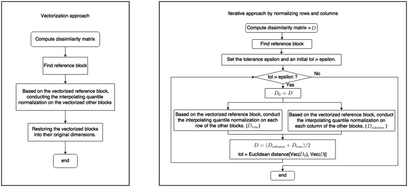
As Figure 1 displays, two normalization approaches have been developed based on the interpolating quantile normalization.

Fig. 1.

Flow charts for the two approaches of dissimilarity matrix correction by the interpolating quantile normalization

• Vectorization: The vectorized other blocks are normalized with respect to the vectorized reference block. Then the normalized vectors are restored as matrices of original dimensions.

• Iterative approach by normalizing rows and columns: In this strategy, the vectorized reference block is again used as the reference vector of the interpolating quantile normalization. In each iteration, denote the matrix before normalizing as D = D₀. Then obtain matrix D_row (D_column) by normalizing each row (column) in all non-reference blocks with respect to the reference vector. Then the dissimilarity matrix D is updated as $D=\frac{1}{2}\left(D_{\text{row}}+D_{\text{column}}\right)$. The iteration will continue until the Euclidean distance between the vectorizations of D and D₀ is smaller than a tolerance number ϵ.

2.5 Clustering and evaluation methods

Standard clustering approaches, such as hierarchical clustering and k-means clustering, are applied to group the subjects after the dissimilarity matrix correction. If the true classification is known, then we can use the adjusted rand index (ARI) to check the agreement between the predicted and the true classification (Hubert and Arabie, 1985). A value close to 1 indicates strong agreement, while a value close to zero indicates poor agreement.

In addition, the area under the receiver operating characteristic (ROC) curve (AUC) is computed for the normalized dissimilarity matrix to evaluate its robustness. It is based on the relations between all pairs of samples. If two samples belong to the same underlying cluster, the pair belongs to the ‘ +’ class. Otherwise, the pair belongs to the ‘−’ class. We then generate the ROC curve using the normalized distance between pairs as the predictor, and the relations between the pairs as outcome and compute the AUC of the ROC curve. This process generates a objective criterion of how well the normalization corrected the unwanted batch effects, without the use of any clustering algorithm. A value closer to 1 suggests better batch effect removal.

3 Results

3.1 Simulation study

Simulation study was conducted to compare the impact of the methods on the accuracy of recapturing true underlying clusters. We compared the two interpolating quantile normalization approaches with ComBat algorithm, which is implemented by Bioconductor package sva (Leek et al., 2012). The interpolating quantile normalization algorithms were implemented by R-package QuantNorm, which is available at https://github.com/tengfei-emory/QuantNorm.

Simulated RNA-seq data that contain six true clusters and three batches were generated by the Bioconductor package PROPER (Wu et al., 2015). The PROPER package generates simulated RNA-seq data based on parameters estimated from true datasets. We generate DE genes to separate the simulated clusters. The three batches have the same sample size but different proportions for each cluster, which were generated from multinomial distribution. In order to produce batch effect, moreover, log over-dispersion and log expression parameters for each gene count in the batches 2 and 3 were assigned fluctuations with respect to the original parameters in the batch 1.

For each combination of parameters, i.e. proportion of DE genes (p.DE), log over-dispersion fluctuations (lOD), log expression fluctuations (lexp) and observed sample size, 40 trials were conducted to compare the ARI obtained by ComBat and the interpolating quantile normalization approaches.

In each of the 40 trials under one set of parameters, a data matrix with three batches was simulated as described. Each batch contributed to one-third of the observed sample size. Then the batch effect correction approaches were performed before the hierarchical clustering. Finally, the ARIs were calculated and the boxplots of the indices were produced to display the performance of various methods.

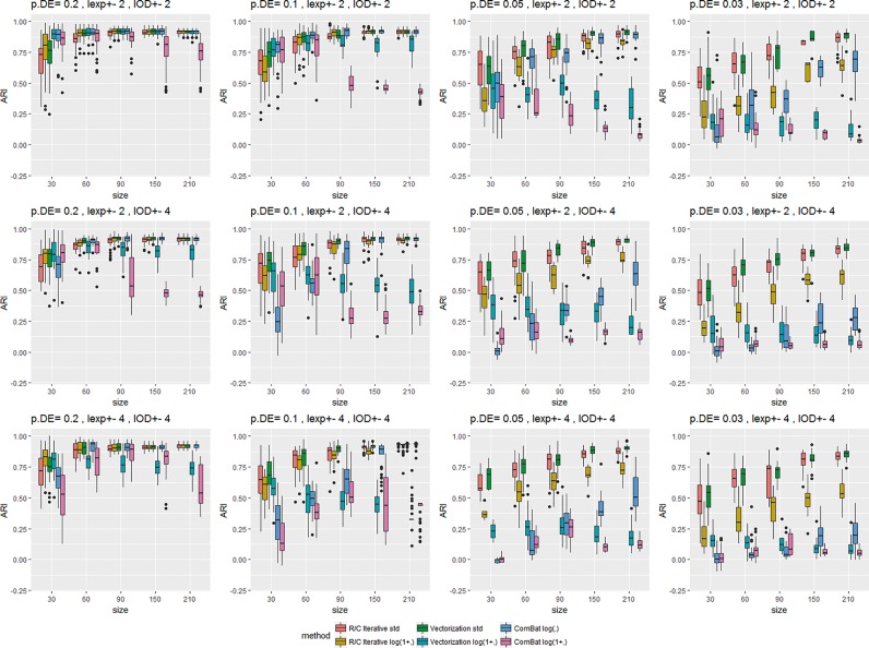
As Figure 2 shows, the performances of most methods improved as the observed sample size increased. Moreover, all methods suffered reduced performances as p.DE decreased and lOD was more fluctuated, where the overlapping between different clusters increased. Compared to quantile normalization methods, ComBat struggled more under difficult situations. In the most difficult case where p.DE = 0.03 and lOD fluctuation = 4 (Fig. 2, lower-right panel), ComBat mostly failed to recapture the true cluster membership, while the interpolating quantile normalization methods could still reach ARIs above 0.5 with reasonably small standard errors. Moreover, when the fluctuation of lexp became larger (Fig. 2, bottom row), ComBat’s performance appeared to be worse but the quantile normalization approaches displayed similar performances as under smaller lexp fluctuations.

Fig. 2.

Simulation results for interpolating quantile normalization methods and ComBat approach based on ARI with respect to different sample sizes, log over-dispersion fluctuations and log expression fluctuations. Std stands for the standardization preprocessing and log($·$) or log(1+$·$) stands for the log-transformation preprocessing

Due to the characteristics of the simulated dataset, the standardization preprocessing boosted the performance of the quantile normalization in most cases, while the log transformation worked better when p.DE was large. However, ComBat was incompatible with the standardization preprocessing so only log transformation was applied for ComBat.

The two quantile normalization methods also displayed different characteristics for different data. When the observed sample size was small (size = 30) and p.DE was large (p.DE = 0.2), i.e. larger number of genes differentiate the clusters, the quantile normalization algorithm with vectorization appeared to perform better than the other two approaches. On the other hand, when the sample size became larger and the p.DE became small, the iterative quantile normalization algorithm showed better performances. Overall, compared to ComBat, the new methods based on dissimilarity matrix quantile normalization achieves better performance in correct re-capturing the true clusters.

In addition, simulations under similar settings were conducted in order to compare our methods and ComBat in terms of the AUC index (Supplementary Fig. S1). The results were similar to the ARI results shown in Figure 2. We further simulated situations where batch effect was non-existent. When the sample size was very small, our methods showed some side effect of over-adjustment. However, the over-adjustment went away when sample size becomes moderate or larger (Supplementary Fig. S2). While there was slightly stronger over-adjustment when the batch effect does not exist and the sample size was very small, our methods were more reliable and robust in most situations where the batch effects were present, which is a more realistic scenario, making it overall a better choice.

In RNA-seq data, sequencing depth can impact the performance of algorithms substantially. We compared the performance by simulating different sequencing depths. Our methods showed consistent advantage at various sequencing depth settings (Supplementary Fig. S3).

We also examined the computing time in the simulation setting. Our method is reasonably fast. As shown in Supplementary Figure S4, the computing time is a few seconds for the vectorization approach and tens of seconds or a few minutes for the iterative approach. More details can be found in the Supplementary Materials.

3.2 ENCODE data for human and mouse tissues

Real data analysis was conducted to evaluate the effectiveness of the proposed methods. 3D principal component analysis (PCA) plots, heatmaps and connection graphs created by R package rgl (Adler et al., 2017), pheatmap (Kolde, 2015), network (Butts, 2015) and ggnetwork (Tyner, 2017) were used to display cluster structures. Package receiver operating characteristic surface (ROCS) (Yu, 2012) was used to compute AUC.

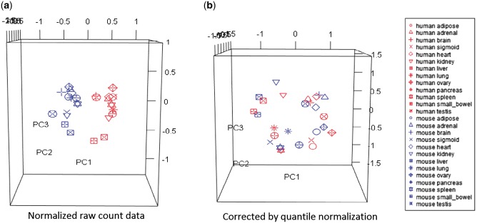
We first re-analyzed the dataset used by Lin et al. (2014) using our methods. We conducted the quantile normalization on the normalized ENCODE raw counts matrix reproduced according to Gilad and Mizrahi-Man (2015), consisting of 10 309 × 26 normalized counts among 13 types of tissues in both human and mouse. As can be seen from the PCA plot before batch effect removal (Fig. 3a), subjects from human (red) were separated from those from mouse (blue). Thus, Lin et al. (2014)’s paper, which ignored the batch effect, concluded that the subjects were clustered by species instead of tissues.

Fig. 3.

3D PCA plots based on (a) the dissimilarity matrix of the normalized ENCODE raw counts data (Gilad and Mizrahi-Man, 2015) and (b) the dissimilarity matrix corrected by the iterative interpolating quantile normalization

In order to correct the batch effect, we applied the iterative quantile normalization approach toward the dissimilarity matrix of the standardized count dataset. It took eight iterations to reach convergence ($\mathrm{ϵ}={10}^{-4}$). As the PCA plot (Fig. 3b) shows, the 26 samples are mainly clustered by tissues. For 12 out of 13 tissues, the closest neighbor after dissimilarity correction was the same tissue in the other organism (Fig. 4). Interestingly, sigmoid still shows big separation based on their organism origin.

Fig. 4.

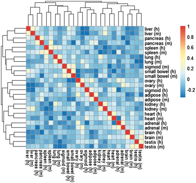
Heatmap for the corrected correlation (1 − dissimilarity) matrix for the normalized ENCODE raw counts data

Compared to the heatmap obtained by ComBat from the same dataset (Fig. 3 in Gilad and Mizrahi-Man, 2015), our method correctly clustered three more pairs of tissues. Hierarchical clustering ARI and the AUC index further confirmed the advantage of our method (ARI = 0.884, AUC = 0.993) over ComBat (ARI = 0.489, AUC = 0.990).

3.3 Human–mouse brain RNA-seq data

Another FPKM matrix dataset of human and mouse brain cells was obtained from Zhang et al. (2016). The data consist of the counts of 15 041 genes in 41 human brain cell samples and 21 mouse brain cell samples. All cell classifications were known, including multiple types of astrocytes, neurons, oligodendrocytes, endothelial and microglia.

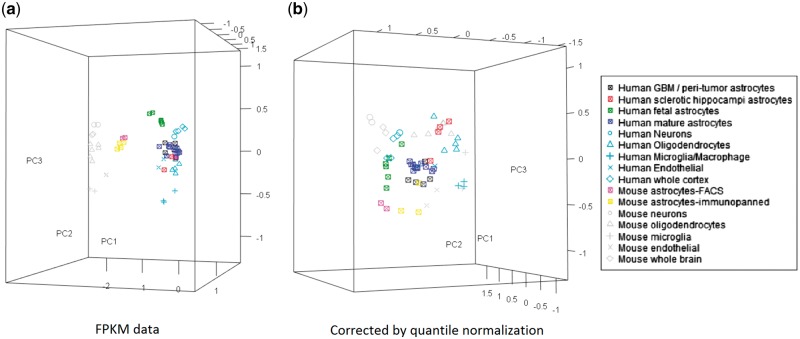
As can be seen from the 3 D PCA plot (Fig. 5a), before correction, the human cells and the mouse cells were separated as two batches. It is of interest whether the same type of cells in human and mouse brain are more similar compared to two different types of cells of human or mouse. Thus, we used the quantile normalization approach to correct the dissimilarity matrix of all 62 subjects in the data, then we used PCA plots to display the similarity of the brain cells in human and mouse.

Fig. 5.

3D PCA plots based on (a) the dissimilarity matrix of the FPKM data (Zhang et al., 2016) and (b) the dissimilarity matrix corrected by the iterative interpolating quantile normalization

The 3 D PCA plot based on the dissimilarity matrices obtained by the iterative quantile normalization approach is shown in Figure 5b. It took 24 iterations to reach the convergence of the Euclidean distance of the dissimilarity matrices between iterations ($\mathrm{ϵ}={10}^{-4}$). After batch effect correction, it can be observed that the oligodendrocytes (triangles), microglia (crosses), whole brain or cortex (diamonds) in human are close to their counterparts in mouse. As expected, the astrocytes (squares with x mark inside) in human brain and mouse brain shows strong diversity based on their origin. The human mature astrocytes and glioblastoma multiforme (GBM) astrocytes form a tight cluster. The six mouse astrocyte samples are distant from the main human astrocyte cluster. The human fetal astrocytes, moreover, form their own cluster, which is closer to the mouse astrocytes. The human sclerotic hippocampi astrocytes are more similar to the oligodendrocytes.

We further constructed a network connection graph between the cell types (Fig. 6). Based on the corrected dissimilarity matrix, the dissimilarity between any pair of cell types was defined as the average dissimilarity between samples belonging to the two types. Then if the dissimilarity between any two cell types was less than 0.2 (25% percentile of the dissimilarity between all pairs), we established a link between them. The graph shows a more complete picture of cell type relations. As shown in Figure 6, the astrocytes from both human and mouse form a tight community in the graph centered around human mature astrocytes, except the human fetal astrocytes. On the other hand, oligodentrocytes from both human and mouse appear to be close to various types of astrocytes. The human and mouse cells tend to connect with their counterparts, which agree with the PCA plots.

Fig. 6.

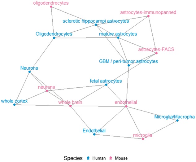
Network connection graph for the brain cells of human and mouse

Correction of the dissimilarity matrix, compared with most existing correction approaches on the raw data, appears to be more reflective of the true connection between cells of different species. One explanation could be that the regulatory networks between genes are more conserved than the expression level of specific genes in evolution. When it comes to different species, the degree of increase or decrease level of a particular downstream gene may differ, but they do play the same biological role. That might be why cells tend to cluster by tissues when we correct the dissimilarity matrix.

3.4 Mouse neuron scRNA-seq data

The mouse neuron RNA-seq dataset GSE59739 (Usoskin et al., 2015) consists of 25 334 features for 622 single mouse neurons. Four groups of cells, namely peptidergic nociceptors (PEP), non-peptidergic nociceptors (NP), neurofilament containing (NF) and tyrosine hydroxylase containing (TH), are evenly distributed among 10 libraries. The libraries could introduce batch effects (Head et al., 2014).

As shown in Figure 7a, using genes that are nonzero in more than 50% of samples, the real biological signal of cell groups was roughly maintained. However, it was insufficient to directly obtain reasonable clustering performance. On the other hand, the distribution of cells among libraries (Fig. 7b) suggests slight variations by libraries. To adjust these small variations, we applied our methods. Figure 7c displays the 3 D PCA plot of the dissimilarity matrix corrected by the iterative approach. As can be seen, our method displayed a clearer pattern of the cell groups in more condensed scales.

Fig. 7.

3D PCA plots based on (a) the dissimilarity matrix of the normalized RPM data (Usoskin et al, 2015) colored by cell groups, (b) the dissimilarity matrix of the normalized RPM data colored by libraries and (c) the dissimilarity matrix corrected by the iterative interpolating quantile normalization

We further calculated the AUC of dissimilarity matrices and average ARI from 100 times of K-means clustering (k = 4) for different methods. Compared to the original normalized RPM data ($\overline{\text{ARI}}$ = 0.312, AUC = 0.847), iterative approach ($\overline{\text{ARI}}$ = 0.726, AUC = 0.867) showed significant improvement. In contrast, ComBat ($\overline{\text{ARI}}$ = 0.289, AUC = 0.796) performed at a similar level as the original data. We note the AUC doesn’t depend on the clustering procedure.

3.5 Human pancreas scRNA-seq data

We applied our method to another scRNA-seq data, GSE85241, of human pancreas (Muraro et al., 2016). The dataset contains 2126 cells, with 19 140 features, from four donors. Similar to the mouse neuron data mentioned above, the samples for this dataset are evenly distributed in eight libraries.

The situation was similar to the mouse neuron data, as the biology variation could be observed from the original data (Fig. 8a). Here again genes that are nonzero in more than 50% of samples were retained. After applying our algorithm, the biological pattern became better separated in more normalized scales (Fig. 8b). Using the same k-means approach as in the previous subsection, the iterative approach ($\overline{\text{ARI}}$ = 0.553, AUC = 0.840) again made reasonable improvement compared to the raw data ($\overline{\text{ARI}}$ = 0.368, AUC = 0.714) and ComBat ($\overline{\text{ARI}}$ = 0.344, AUC = 0.692).

Fig. 8.

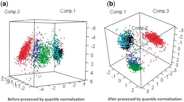
PCA plots based on (a) raw data (Muraro et al., 2016) and (b) dissimilarity matrix obtained by the interpolating quantile normalization. Colors refer to the cell types

4 Discussion

Adjusting for batch effect is important when conducting clustering analysis for the RNA-seq data. In this paper, we proposed novel approaches based on the interpolating quantile normalization. As the data become challenging, i.e. true clusters are closer to each other, and the batch effect is heterogeneous on different clusters, our methods outperform ComBat. However, we should point out that ComBat is a more general method, which adjusts the data matrix for many kinds of down-stream analysis, while our method focuses on adjusting the dissimilarity matrix between samples, mainly serving the purpose of pattern detection in the samples. It does not correct the raw count matrix to adjust for batch effects.

Our method provides a bridge, the corrected dissimilarity matrix, between raw data and clustering and other pattern detection techniques. Instead of directly conducting clustering, our method modifies the dissimilarity matrix so that various clustering approaches can achieve better performance. Although we mainly used hierarchical clustering and k-means clustering to illustrate the performances, our method can also be combined with other clustering approaches. For instance, using the dissimilarity matrix corrected by our method, the powerful SC3 method (Kiselev et al., 2017) achieves average ARIs of 0.933 (SD = 0.003) and 0.926 (SD = 0.020) for the mouse neuron data (Usoskin et al., 2015) and the human pancreas data (Muraro et al., 2016) respectively, among 100 repeated runs. Notice that the corrected dissimilarity stayed the same, as our method is deterministic. The stochastic aspect of the results came from SC3. As shown in Supplementary Figure S5, these results were better and more robust compared to the results obtained by SC3 using the uncorrected distance matrices [$\overline{\text{ARI}}$ = 0.872 (SD = 0.020); $\overline{\text{ARI}}$ = 0.833 (SD = 0.100)].

There are some limitations in our methods. Because the interpolating quantile normalization will map the full range of the reference vector to the target vector, a vector with very small variance can be normalized into a polarized vector. Although the polarization can magnify the decreased pattern signal in the between-batch blocks, it may also produce extreme patterns which do not exist. This characteristic of quantile normalization has side effects for both our methods. On the one hand, the vectorization approach may suffer from insufficient discrimination due to the lack of extreme values. On the other hand, the row/column iterative approach is more easily affected by the wrong extreme values since each column and each row are polarized. Therefore, the vectorization approach performed better on data with high similarity between batches, such as the ENCODE data, while the iterative approach was more suitable for more irregular and imbalanced data, such as the human–mouse brain data.

In addition, the preprocessing method can affect the result of the clustering analysis. The dissimilarity matrix can be different after standardization or log-transformation, especially in the sense of the relative orders of the entries. So the final product of matrix correction will also be different. Both simulation and real data analysis have shown that the choice of the two preprocessing strategies may depend on data, as we utilized standardization for the ENCODE data and log-transformation for the human–mouse brain RNA-seq data.

Although the iterative approach seems to have limitations explained earlier, we generally recommend this approach. This is because there are saddle-point-like entries existing in the dissimilarity matrices, which may cause confusing interpretations in terms of the distance between samples. Compared to the vectorization approach, which retains the order of entries within each block, the iterative approach reallocates the extreme values to the ’hidden’ local extremes instead of the false saddle points. This mechanism can improve the robustness of the algorithm and restore the hidden patterns in the dissimilarity matrix.

Funding

This work was partially funded by NIH [grant numbers R01GM124061, R37AI051231 and U19AI057266] and Natural Science Foundation of China [grant numbers NSFC41476120 and NSFC41676119].

Conflict of Interest: none declared.

References

- Adler D. et al. (2017) Rgl: A r-library for 3d visualization with opengl. Proceedings of the 35th Symposium of the Interface: Computing Science and Statistics, Salt Lake City. Vol. 35. 2003.
- Benito M. et al. (2004) Adjustment of systematic microarray data biases. Bioinformatics, 20, 105–114. [DOI] [PubMed] [Google Scholar]
- Butts C.T. (2015) network: a Package for Managing Relational Data in R. Journal of Statistical Software, 24.2, 1–36. [Google Scholar]
- Chen C. et al. (2011) Removing batch effects in analysis of expression microarray data: an evaluation of six batch adjustment methods. PLoS One, 6, e17238. [DOI] [PMC free article] [PubMed] [Google Scholar]
- Gagnon-Bartsch J.A., Speed T.P. (2012) Using control genes to correct for unwanted variation in microarray data. Biostatistics, 13, 539–552. [DOI] [PMC free article] [PubMed] [Google Scholar]
- Gilad Y., Mizrahi-Man O. (2015) A reanalysis of mouse ENCODE comparative gene expression data. F1000Res., 4:121. [DOI] [PMC free article] [PubMed] [Google Scholar]
- Head S.R. et al. (2014) Library construction for next-generation sequencing: overviews and challenges. Biotechniques, 56, 61. [DOI] [PMC free article] [PubMed] [Google Scholar]
- Hubert L., Arabie P. (1985) Comparing partitions. J. Classification, 2, 193–218. [Google Scholar]
- Johnson W.E. et al. (2007) Adjusting batch effects in microarray expression data using empirical Bayes methods. Biostatistics, 8, 118–127. [DOI] [PubMed] [Google Scholar]
- Kiselev V.Y. et al. (2017) SC3: consensus clustering of single-cell RNA-seq data. Nat. Methods, 14: 483–486. [DOI] [PMC free article] [PubMed] [Google Scholar]
- Kolde R. (2015) Pheatmap: pretty heatmaps. R package version 1.0.8. https://cran.r-project.org/web/packages/pheatmap/pheatmap.pdf.
- Leek J.T. et al. (2012) The sva package for removing batch effects and other unwanted variation in high-throughput experiments. Bioinformatics, 28, 882–883. [DOI] [PMC free article] [PubMed] [Google Scholar]
- Lin S. et al. (2014) Comparison of the transcriptional landscapes between human and mouse tissues. Proc. Natl. Acad. Sci. USA, 111, 17224–17229. [DOI] [PMC free article] [PubMed] [Google Scholar]
- Müller C. et al. (2016) Removing batch effects from longitudinal gene expression-quantile normalization plus combat as best approach for microarray transcriptome data. PLoS One, 11, e0156594. [DOI] [PMC free article] [PubMed] [Google Scholar]
- Muraro M.J. et al. (2016) A single-cell transcriptome atlas of the human pancreas. Cell Syst., 3, 385–394. [DOI] [PMC free article] [PubMed] [Google Scholar]
- Stephanie C. et al. (2015) Missing data and technical variability in single-cell RNA-sequencing experiments, Biostatistics, kxx053, https://doi.org/10.1093/biostatistics/kxx053. [DOI] [PMC free article] [PubMed]
- Sudmant P.H. et al. (2015) Meta-analysis of RNA-seq expression data across species, tissues and studies. Genome Biol., 16, 287. [DOI] [PMC free article] [PubMed] [Google Scholar]
- Tyner S. (2017) Network Visualization with ggplot2. R Journal, 9.1.
- Usoskin D. et al. (2015) Unbiased classification of sensory neuron types by large-scale single-cell RNA sequencing. Nat. Neurosci., 18, 145–153. [DOI] [PubMed] [Google Scholar]
- Wu H. et al. (2015) PROPER: comprehensive power evaluation for differential expression using RNA-seq. Bioinformatics, 31, 233–241. [DOI] [PMC free article] [PubMed] [Google Scholar]
- Yu T. (2012) ROCS: receiver operating characteristic surface for class-skewed high-throughput data. PLoS One, 7.7, e40598.. [DOI] [PMC free article] [PubMed] [Google Scholar]
- Zhang Y. et al. (2016) Purification and characterization of progenitor and mature human astrocytes reveals transcriptional and functional differences with mouse. Neuron, 89, 37–53. [DOI] [PMC free article] [PubMed] [Google Scholar]
Associated Data
This section collects any data citations, data availability statements, or supplementary materials included in this article.