The use of matched molecular series networks for cross target structure activity relationship translation and potency prediction

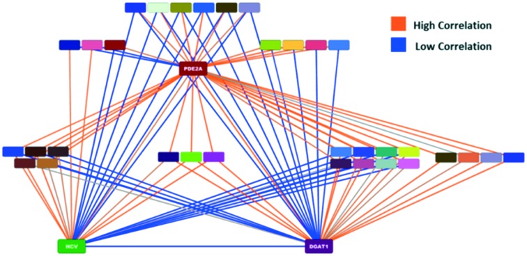
Matched molecular series (MMS) network for PDE2A, DGAT1, and HCV showing the relationships between shared MMS/target combinations.

Abstract

Matched molecular series (MMS) analysis is an extension of matched molecular pair (MMP) analysis where all of the MMPs belong to the same chemical series. An MMS within a biological assay is able to capture specific structure activity relationships resulting from chemical substitution at a single location in the molecule. Under this convention, an MMS has the ability to capture one specific interaction vector between the compounds in a series and their therapeutic target. MMS analysis has the potential to translate the SAR from one series to another even across different protein targets or assays. A significant limitation of this approach is the lack of chemical series with a sufficient number of overlapping fragments to establish a statistically strong SAR in most databases. This results in either an inability to perform MMS analysis altogether or a potentially high proportion of spurious matches from chance correlations when the MMS compound count is low. This paper presents the novel concept of an MMS Network, which captures the SAR relationships between a set of related MMSs and significantly enhances the performance of MMS analysis by reducing the number of spurious matches leading to the identification of unexpected and potentially transferable SAR across assays. The results of a full retrospective leave-one-out analysis and randomization simulation are provided, and examples of pharmaceutically relevant programs will be presented to demonstrate the potential of this method.

Introduction

The pursuit of compounds with a desired activity profile is the essence of medicinal chemistry and is the motivation for building structure activity relationships (SARs). Oftentimes, the SAR reflects an association between a small and structurally similar series of compounds and their pharmacological activity against one particular therapeutic target (i.e. a local SAR). The goal of the local SAR is to reveal critical interaction properties that aid in the rational design of analogs that improve potency.

Given the vast amount of available SAR information across many targets spanning many years, especially within large pharmaceutical companies, there has been considerable effort to extract knowledge from this data for compound design across series within a target, and even across targets. In recent years, matched molecular pair (MMP) analysis has been extensively evaluated and has shown some success in predicting physicochemical properties.1,2

Unfortunately, success in predicting biological activity has been far more limited. When an MMP transformation includes activity from multiple targets, the potency change is, generally, normally distributed around zero.3 Limiting the transformation to data from a single target may overcome this issue, however, the number of underlying compounds is reduced and potentially weakens the conclusions one can draw. Furthermore, limiting an analysis to data for a single target focuses on a narrow chemistry space and will ultimately limit the breadth of MMP transformations that will be generated. Another issue with MMP analysis is the need to define the appropriate structural context for a transformation.4 This can be difficult to do a priori and can result in too few pairs for analysis.

Recently, MMP analysis has been logically extended to the concept of matched molecular series (MMS) analysis, a term introduced by Wawer and Bajorath.5 An MMS is a series of compounds in which all members share the same core and differ by changes at a single position. By definition, any two compounds within an MMS are MMPs of one another. Furthermore, an MMS can be connected to changes in the activity of its constituent compounds for a particular assay. The approach of using MMS for biological SAR transfer has been reported6–11 and is the basis for methods such as Matsy,12 which begins to address the question of “what to make next?”. The attraction of MMS as an approach for compound design is its intuitively familiar concept of extracting trends and knowledge from prior series and applying them to the design of novel analogs during a lead optimization process.

The premise of the MMS approach is this: given a sufficiently strong activity correlation, analogs present in one MMS series that are not present in a second MMS series may contain candidate fragments worthy of evaluating in the second series. This parallel SAR approach is analogous to the concept of “sub-pocket fingerprints”13,14 where, despite comparing two distinct biological targets, there are regions in their respective binding pockets that are similar. The underlying assumption is that the fragments of the two MMSs bind to their respective sub-pockets via similar binding interactions. An early success of this approach was reported by Mills et al. for the design of TRPA1 antagonists.15

On the surface, conducting an MMS analysis is fairly straightforward. Start with a congeneric series of compounds (Query MMS) and search for other series that possesses an overlapping set of fragments to the query (Match MMS). If the activities of the overlapping fragments common to a Match MMS and the Query MMS are correlated, then we call that an MMS pair. It is important to note that the two MMS series could have activity from the same or different assays and an MMS could correlate with multiple MMS series from different assays or targets.

While this concept is simplistic in its approach, in practice, many details need to be managed. Given the large amount of biological data with many possible MMS series, the potential of finding a highly correlated MMS pair by chance alone is high, and the likelihood of this chance correlation increases with decreasing number of corresponding fragments. Clearly, an MMS pair with many corresponding analogs (i.e. >10 fragments) is desirable as it decreases the potential for chance correlation and increases the potential of a true parallel SAR. However, MMS pairs with many overlapping fragments are not common and pragmatism leads to the analysis of MMS pairs with a small number of fragments. Relaxing the required number of corresponding analogs for the MMS pair (i.e. 5–10 corresponding fragments) greatly increases the number of MMS pairs and subsequent predictions; however many of these MMS pairs are likely spurious matches, correlated by chance, where a true parallel SAR may not exist. Kramer et al.16 have performed an analysis of metrics for determining MMS similarity in order to identify those that result in the best activity prediction.

In this paper, we describe how an MMS pair can be used for activity prediction and assess performance on the Pfizer MMP database. We also assess the likelihood of chance correlations in a typical analysis via a random shuffle experiment. Finally, we introduce the concept of a network representing the SAR between an interrelated group of matched molecular series (MMS Network) and show how this concept can be used to address the issue of chance correlations and identify unexpected and potentially transferable SAR across assays.

Methods

Data set

The data used in this analysis are Pfizer's in-house IC₅₀, K_i, and EC₅₀ potency endpoints, with some basic filters applied. All data were transformed to pActivity values (–Log₁₀ (Activity)). Individual measurements outside the pActivity range 3–12 were removed from the analysis, as were assays having less than 10 data points and a pActivity range less than 1.0. This resulted in 5 350 628 data points spanning 7759 assays.

Identification of MMSs

Matched molecular series were identified from the Pfizer matched molecular pair (MMP) database described previously.17 An MMS is defined as a congeneric series with a minimum of 5 compounds that are all MMPs of one another. The variable fragment must have 10 or fewer non-halogen heavy atoms if it is a substituent (1 bond break) and 12 or fewer non-halogen heavy atoms if it is a core (2 or 3 bond-breaks).

Identification of correlated MMS SAR

MMS pairs were identified by a systematic comparison of MMSs. To ensure robustness of the MMS pairs, each candidate MMS was required to have a range of pActivity ≥ 0.5 and a skew ≤3.0. These filters reduce the risk of chance correlations and linear relationships driven by extreme outliers. The linear relationship between MMS pairs was computed using orthogonal regression. This method is also called Deming regression, where δ = 1,18 and is a form of total least squares (TLS) regression.19 An advantage of orthogonal regression is that it accounts for assay variability in both the x and y regression dimensions. MMS pairs with an orthogonal regression slope outside the range of 0.2–5.0 and a squared Pearson correlation coefficient <0.16 were removed from further analysis. It is important to note that these are preliminary filters applied before additional consideration of the MMS pairs.

QSAR predictions

To make predictions from one MMS to another, the orthogonal regression relationship is used. Consider, for example, a query series Q and a matching series M. Given a fragment i in M, with activity M_i, its predicted activity in Q, Q[combining circumflex]_i, can be computed from the equation:Q[combining circumflex]_i = slope × M_i + interceptwhere the slope and intercept are computed from the orthogonal regression of all activity data for the fragments Q and M have in common.

Graph DB

The MMS pair graph database was constructed using Neo4J.20 In this graph database, the nodes represent individual MMSs, and the edges between nodes represent the correlation statistics of the MMS pair. Note that not all pairs of nodes have an edge due to inadequate overlap of fragments or the filtering of MMSs described previously. The edge correlation statistics stored are the squared Pearson's correlation coefficient (R²) and the p-value of the correlation. The p-values are based upon the null hypothesis that the true correlation coefficient is 0.0, meaning that smaller p-values represent correlations that are statistically different from 0.0. The final database contained ∼281 000 nodes and ∼36 million edges.

MMS network analytics

The support for an individual match (edge) was computed from the graph database by analyzing all sets of 3 nodes and edges where two of the nodes (N1 and N2) represent the MMS pair being analyzed and the third node (N3) represents a different MMS that is correlated to at least one of N1 and N2. For this analysis, a pair of nodes is considered to be correlated if the square of their Pearson correlation coefficient (R²) ≥ 0.49. This is an arbitrary value that was chosen based on empirical observations from our data sets. Cases where the third node is not correlated (R² < 0.49) to either of the first two were not included since they do not add any support for or against the original SAR correlation. The MMS network graph scores computed for an MMS pair are the average N1–N3 and N2–N3 R² over all sets, and the average N1–N3 and N2–N3 p-value over all sets. Note that these average values are MMS network support scores and no longer represent actual correlations or p-values.

Leave-one-out (LOO) analysis

To evaluate prediction performance, a leave-one-out analysis was performed by removing every pair of compounds with the same fragment within a MMS pair one at a time. Correlation metrics and linear regression parameters were then recomputed on the N-1 remaining fragments and a prediction made for each of the left out compounds. For the network metrics, the compound being predicted was left out of all MMS network metric calculations.

Results & discussion

Single MMS pair predictions

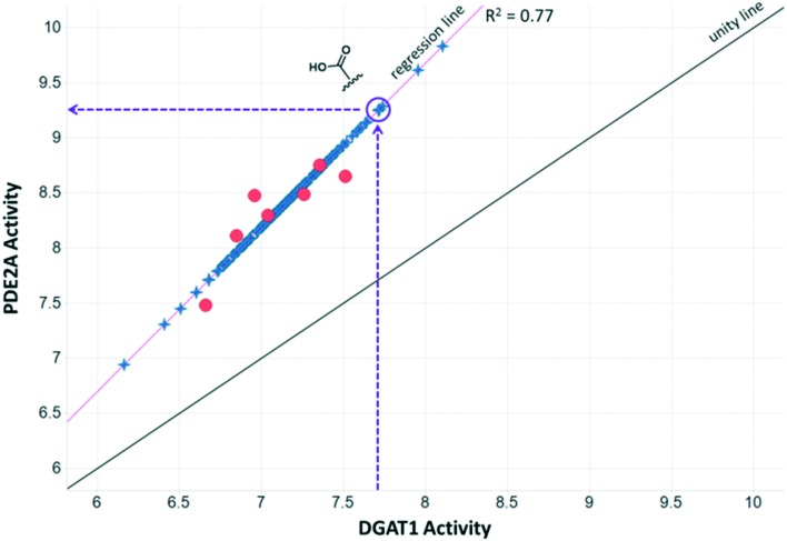
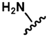
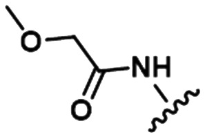
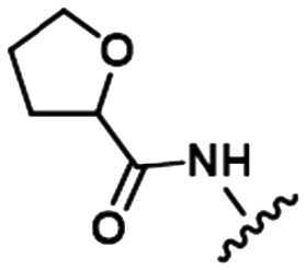
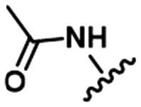
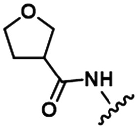
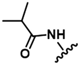
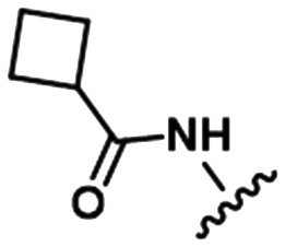
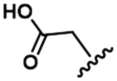
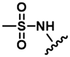
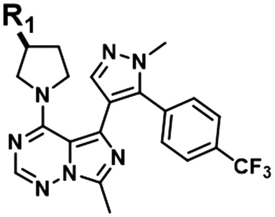
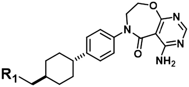
To illustrate the utility of MMS pair analysis for prospective potency prediction, we first present an example from a comprehensive leave-one-out (LOO) analysis performed on the Pfizer database. The first row of Table 1 contains the SAR of our query MMS, a series of nine, structurally-diverse phosphodiesterase 2A (PDE2A) inhibitors.21,22 A search of the Pfizer database identified a series of acyl-CoA:diacylglycerol acyltransferase-1 (DGAT1) compounds23–25 as an MMS match, shown in the second row of Table 1. Note that although the scaffold of the two MMSs is quite different, seven of the nine fragment substitutions are the same. To investigate the relationship between these two MMSs, their respective activities were plotted. Each point in Fig. 1 represents the activity data for a pair of compounds bearing the same fragment; DGAT1 activity on the x-axis and PDE2A activity on the y-axis. The similarity of the two SARs can be quantified using the square of the Pearson's correlation coefficient (R²), which in this case is 0.77 and indicates a strong agreement for this MMS pair. The linear fit between the two MMSs is computed using orthogonal regression (magenta line). The unity line in Fig. 1 highlights the absolute activity differences of the two assays, PDE2 activity being higher than DGAT activity across the board. Both the slope and relative range of potencies can be different, however this has no bearing on the correlation of the respective SARs.

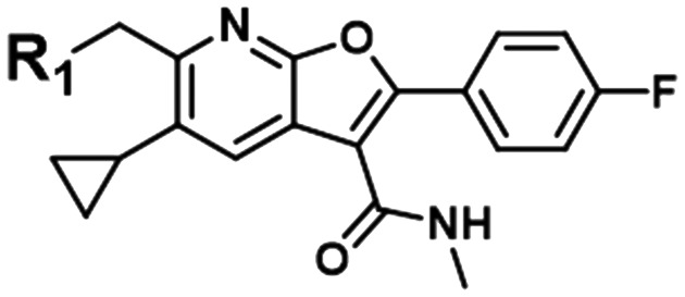
Table 1. Examples of matched molecular series (MMS) with associated pIC₅₀ data in PDE2A (1), DGAT1 (2), and HCV (3).

	Core	Assay
1		PDE2A	7.5	8.0	8.1	8.3	8.4	8.5	8.5	8.7	8.8
2		DGAT1	6.7		6.9	7.0		7.0	7.3	7.5	7.4
3		HCV	5.2	5.5		6.2	5.6				6.3

Fig. 1. Plot of PDE2A pIC₅₀ values vs. DGAT1 pIC₅₀ values where each orange circle represents the data for a particular fragment in the MMSs. The line of unity is shown in black and the orthogonal regression line is shown in magenta. Compounds with additional data in the DGAT1 MMS are shown as blue stars and plotted on the regression line. The regression line can be used to make predictions of PDE2A activity for fragments that were screened in the DGAT1 assay as shown for the carboxylic acid fragment.

To leverage the DGAT1 MMS match and identify novel fragments for the PDE2A MMS, we must first identify additional compounds from the DGAT1 series that have measured activity data. These compounds are shown as blue stars in Fig. 1, plotted on the orthogonal regression line. To predict the PDE2A activity for these fragments, the linear orthogonal regression fit can be used. Take, for example, the highlighted carboxylic acid group as our first LOO fragment. The DGAT1 analog bearing this fragment has a pIC₅₀ of 7.7 (vertical, purple dashed arrow), which corresponds to a predicted PDE2A pIC₅₀ of 9.2 (horizontal, purple dashed arrow). The experimentally measured PDE2A pIC₅₀ for this compound is 9.0. This is an example of an MMS pair with good correlation and apparent translatable SAR. Fig. 1 also shows many other compounds, with varying degrees of DGAT1 activity, which were never made or tested in the PDE2A series. All of these represent potential ideas that could be made for PDE2A depending on the needs of the project.

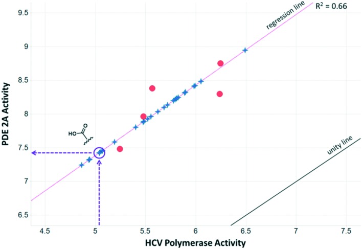
The PDE2A-DGAT1 example represents only one potential match for the PDE2A MMS. A second example is the MMS shown in the third row of Table 1, a series of Hepatitis C virus RNA polymerase (HCV) data26 with five fragments matching the PDE query MMS. Fig. 2 shows the data for the matching fragment compounds (orange circles) and all other compounds (blue stars) with measured pIC₅₀ values in the HCV assay. This MMS pair also has good statistics with a correlation R² of 0.66 and a good range and distribution of activities in both assays. In the HCV assay, the carboxylic acid analog had a measured pIC₅₀ of 5.1, well below the pIC₅₀ of the five matching fragments. This corresponds to a predicted pIC₅₀ of 7.4 in PDE2A, which is significantly lower than the experimental pIC₅₀ of 9.0. For this particular match, the activity data for the carboxylic acid compound does not appear to align with the rest of the SAR in these series. This could occur for a couple of reasons. One explanation is that the experimental measurements from one or both series are suspect, leading to a false correlation or a false prediction. Another possibility is that the data is correct, but that the underlying SARs are not a true match. This can happen when there are a limited number of common fragments used to calculate the correlation. Both of these scenarios can lead to chance (non-causal) correlations.

Fig. 2. Plot of PDE2A pIC₅₀ values vs. HCV pIC₅₀ values where each orange circle represents the data for a particular fragment in the MMSs. The line of unity is shown in black and the orthogonal regression line is shown in magenta. Compounds with additional data in the HCV MMS are shown as blue stars and plotted on the orthogonal regression line. The location of the carboxylic acid fragment and its prediction in PDE2A is shown.

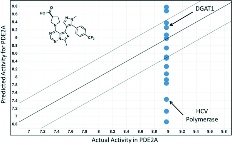
A closer examination of the full set of 16 predictions made for the PDE2A carboxylic acid compound highlights a potential issue with this approach. Fig. 3 shows a plot of the predicted vs. experimental pIC₅₀ values for the PDE2A carboxylic acid compound resulting from the 16 matching MMSs. The predicted pIC₅₀ values range from 6.9 to 9.8 and 10 of 16 fall outside of 3-fold error – our definition of an acceptable prediction. For a project team hoping to use this approach prospectively, there would be no means to know which, if any, of the predictions are accurate.

Fig. 3. MMS predicted vs. actual pIC₅₀ values for the carboxylic acid analog in PDE2A. Note the large range of predictions (6.8–9.8).

Overall MMS match prediction performance

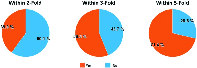
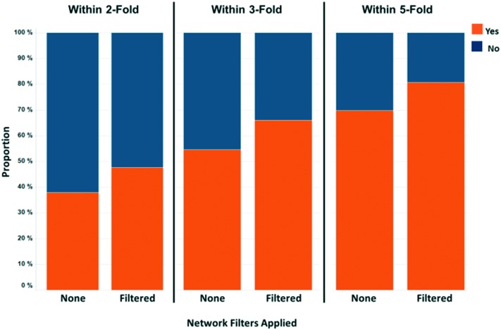
To assess the overall performance of predictions using this simple MMS matching scheme, we performed a full leave-one-out (LOO) analysis of the MMS pairs in the Pfizer database. We restricted MMS pair matches to those with 6 or more fragments, then left out one fragment at a time and computed the correlation statistics for the remaining fragments. The number 6 was arbitrarily chosen to ensure that there were enough fragments to detect an SAR relationship while ensuring that there were enough MMS pairs to analyze in the overall data set. We used the orthogonal regression line to predict the activity for the leave-out fragment compound in each of the MMS pair assays. This resulted in 569 million LOO predictions. 214 million of those predictions met a set of minimal filtering criteria, defined as: 1) an MMS pair squared Pearson's correlation (R²) ≥ 0.16, 2) an activity range ≥0.5 for both assays, 3) an absolute orthogonal regression slope between 0.2 and 5.0, and 4) an absolute skew ≤3.0 for the compound activities in both assays. These filters represent our minimum requirements for a match to be considered potentially biologically meaningful. To analyze overall performance, we selected a random 1 million results from the 214m predictions and then further filtered this set to those predictions with an R² ≥ 0.49 to identify those generated from a strongly correlated match. This filtering resulted in 363k predictions, or 36.3% of the 1 million randomly selected predictions, which we will call the ‘Analysis Set’. Fig. 4 shows the proportion of the Analysis Set within 2-fold (39.9%), 3-fold (56.3%), and 5-fold (71.4%) of the experimental values.

Fig. 4. Analysis set prediction performance where orange segments show the proportion of predictions within 2, 3, and 5-fold of their actual value.

Likelihood of chance correlations

To assess the likelihood of chance correlations, we performed a randomization experiment to determine the random probability of finding matches with a high correlation. The activity values for each MMS in an MMS pair were randomly shuffled prior to computing the leave-one-out correlation statistics and the minimal filtering criteria were applied, leaving 166m of the 569m total LOO predictions. As with the non-random case, we sampled 1m of these predictions and applied the R² ≥ 0.49 criteria to select only those having a strongly correlated match. This filtering resulted in 291k predictions, or 29.1% of the 1 million randomly selected predictions, which we will call the ‘Random Analysis Set’.

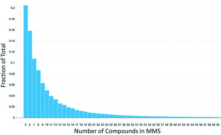
One striking observation is that the non-random experiment had 36.3% strongly correlated MMS pairs and the random experiment had 29.1% strongly correlated MMS pairs. This suggests that as many as 80% could be due to chance alone. This result is not entirely unexpected considering the limited number of matching compounds and data underlying a majority of the correlation calculations, as well as the total number of calculations being performed. A distribution of the number of fragments (minimum of 5) per MMS found in the full Pfizer database is shown in Fig. 5. 57.5% of the MMSs contain 7 or fewer fragments which limits the number of MMSs that can be used with high confidence to a smaller number of series.

Fig. 5. Distribution of MMS compound counts for all MMS with 5–50 compounds in the Pfizer database.

MMS network analysis

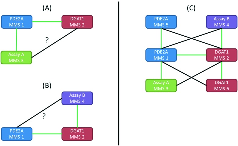
To better discriminate predictions originating from truly correlated SAR from predictions resulting from chance correlation, we returned to the underlying hypothesis of the approach: correlations exist between series that share the same underlying SAR at the position where the change is occurring. This led us to consider what additional information could we learn from other correlations that the MMSs in the MMS pair being analyzed have in common since they should also represent the same or similar SAR? This relational concept is depicted in greater detail in Fig. 6. In the case of the PDE2A-DGAT1 MMS pair (MMS 1 and MMS 2 respectively), consider the hypothetical MMS containing a third chemical series, MMS 3, with activity from Assay A, which is correlated to MMS 1 of PDE2A. If that correlation is due to truly shared SAR, then MMS 3 of Assay A should also be correlated to MMS 2 of DGAT1, assuming they share overlapping fragments. This relationship is represented graphically in Fig. 6A. If MMS 3 is also correlated to MMS 2, one could argue that strengthens the validity of the PDE2A-DGAT1 SAR correlation since there are now three different MMSs that appear to share an SAR. If MMS 3 is not correlated to MMS 2, then support for the PDE2A-DGAT1 match is weakened. Similarly, if a hypothetical MMS with a fourth chemical series, MMS 4 of Assay B, is correlated to MMS 2 of DGAT1, then it should also be correlated to MMS 1 of PDE2A (Fig. 6B). If this is the case, the PDE2A-DGAT1 match is further strengthened, and if not, the match is further weakened. Note that Assay A and/or Assay B could be different biological systems relative to PDE2A or DGAT1. Alternatively, the MMSs correlated to PDE2A or DGAT1 (MMS 5 and MMS 6) could also be different structural cores screened within the same PDE2A or DGAT1 assay (Fig. 6C).

Fig. 6. MMS sets where the strength of the relationships shown in black can be used to determine the support for the initial SAR relationship. If the black edges represent strong SAR correlations, then it supports the original hypothesis, if they represent poor SAR correlations then they detract from the original hypothesis. (A) Case where there is another MMS (MMS 3) correlated to the PDE2A MMS (MMS 1). (B) Case where there is another MMS (MMS 4) correlated to the DGAT1 MMS (MMS 2). (C) Overall MMS network generated from combining all instances of (A) and (B). Note that additional MMSs can be from different (MMS 3 and 4) or the same (MMS 5 and 6) assay as the original MMSs.

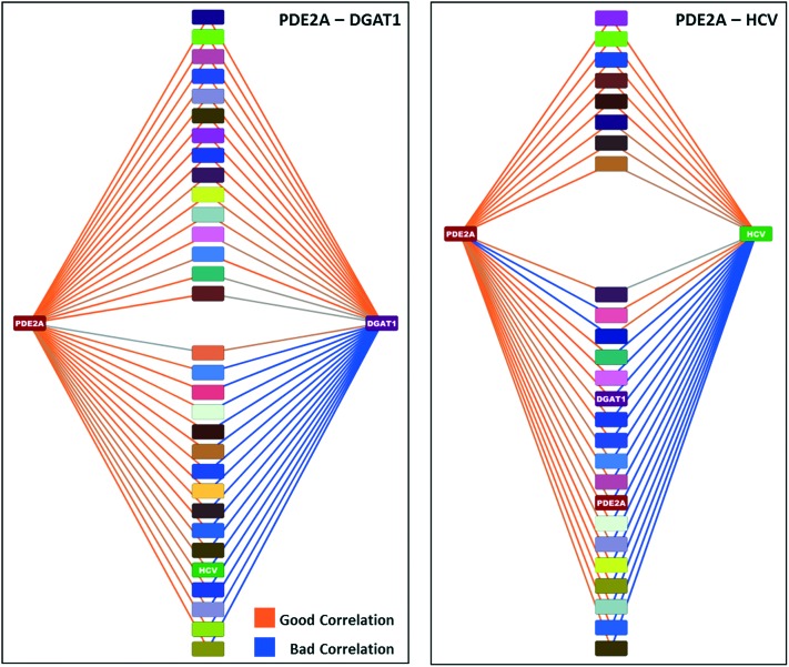
The network graph for the PDE2A-DGAT1 match is shown in the left side of Fig. 7. In this network, the nodes are colored by assay and the edges are colored by the p-value of the correlation between the nodes (null hypothesis that correlation is zero). Orange colored lines represent edges with a low p-value (good correlation), while blue colored lines represent edges with a high p-value (bad correlation). There are 15 MMSs with activities in other assays that are correlated to both the PDE2A and DGAT1 MMSs, as shown in the upper half of the plot. In addition, there are 16 MMSs that are correlated to either the PDE2A or DGAT1 MMSs, but not both. These are shown in the bottom half of the plot. If we compare the PDE2A-DGAT1 network graph to the PDE2A-HCV network graph, shown in the right side of Fig. 7, we observe a striking difference. Only 8 MMSs are highly correlated to both the PDE2A and HCV MMSs and 18 MMSs are highly correlated to only one. For these 2 cases, we would qualitatively argue that the MMS network support for the PDE2A-DGAT1 match is stronger than the MMS network support for the PDE2A-HCV match.

Fig. 7. MMS network for the PDE2A-DGAT1 (left) and PDE2A-HCV (right) examples. The nodes in the center of each plot represent MMSs that are correlated to either PDE2A and/or DGAT1/HCV.

To quantify this difference, we can compute a set of MMS network scores. For this, we use the mean R² and p-value for all of the edges between the original MMS pair and additional matching MMSs as scores for the match. Note that these values can no longer be interpreted as correlation coefficients or p-values, but simply as MMS network support scores for the edge being analyzed.

Scoring predictions

Using the MMS network approach, we can now score the set of predictions for the carboxylic acid analog in the PDE2A example. For the DGAT1 prediction, the MMS network average p-value and R² are 0.18 and 0.50, respectively. For the HCV prediction, the MMS network average p-value is higher at 0.23 and the average R² is lower at 0.46, which is consistent with the qualitative interpretation of the MMS network images in Fig. 7.

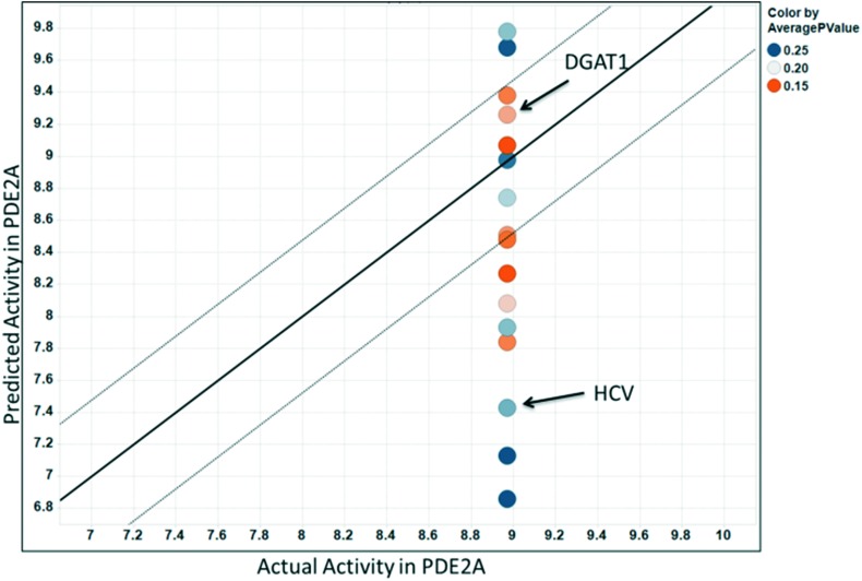
Fig. 8 shows all of the predictions shown in Fig. 3, now colored by their average MMS network p-value scores. This shows that most of the predictions with greater than 3-fold error have higher scores (lower network support) than the predictions with lower than 3-fold error. In practice, to identify the predictions with the highest likelihood of success, one could filter the predictions using the network scores, chose the prediction with the best network score, or perform a weighted average prediction where each prediction is weighted by its MMS network support.

Fig. 8. Predicted vs. actual pIC₅₀ values for the carboxylic acid analog in PDE2A. Each point is colored by its MMS network average p-value score. Predictions with greater network support are colored in orange while predictions with lower support are blue.

Overall network match performance

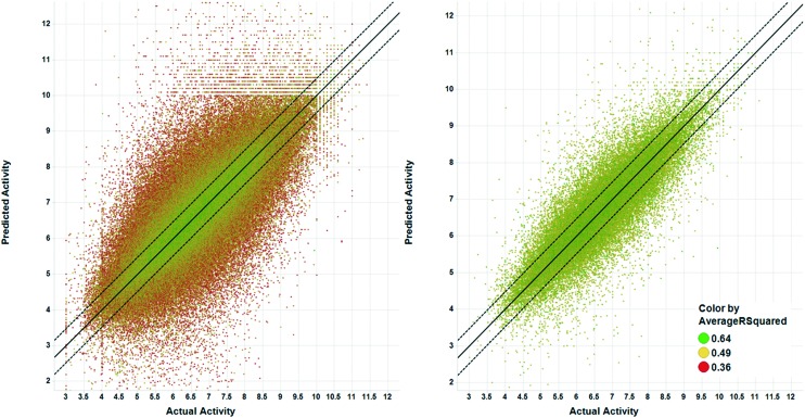
To assess the overall prediction performance when taking MMS network scores into account, we filtered the original Analysis Set by removing predictions with an average network p-value score > 0.2 and an average network R² < 0.49. After filtering, 58k (16%) of the original 363k predictions with a high R² remained. Fig. 9 shows the proportion of predictions within 2, 3, and 5 fold of the actual values. For all cases, the proportions increased compared to the full set: from 38.0% to 47.7% for 2-fold, 54.6% to 66.1% for 3-fold and 69.9% to 80.8% for 5-fold. It is clear that removal of predictions with no or poor MMS network support results in significantly increased prediction accuracy. Fig. 10 shows the predicted vs. actual plots before and after network filtering. The points are colored by their average MMS network R² value.

Fig. 9. Analysis set prediction performance comparison before and after filtering to predictions with MMS network average p-value scores ≤ 0.2 and average R² scores ≥ 0.49.

Fig. 10. Predicted vs. actual values for analysis set predictions. Right plot shows the results after filtering to predictions with MMS network average p-value scores ≤ 0.2 and average R² scores ≥ 0.49. Points are colored by the MMS network average R² score. Solid line is line of unity and dashed lines represent ±3 fold error.

False discovery rate using MMS network approach

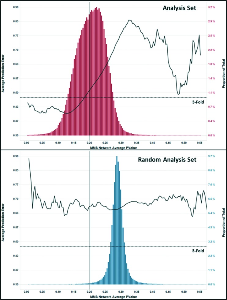
To confirm that the use of MMS network scoring helps to discriminate between real and chance correlations, we built an MMS network for the randomly shuffled data set that showed a high number of good correlations even after shuffling the activities. We then computed MMS network average p-value and R² scores for the predictions in the Random Analysis Set. Fig. 11 shows a comparison of the MMS network p-value score distributions for the Analysis Set and Random Analysis Set. There is a significant right shift of the p-value score distribution for the Random Analysis Set with only 0.97% of predictions falling below the 0.20 threshold, compared to 45.8% of predictions falling below that same threshold for the Analysis Set. This demonstrates that although a large proportion (29%) of chance correlations was found in the full random analysis data set, they are almost completely eliminated (0.28%) by the MMS network filtering.

Fig. 11. Plots of MMS network average p-value distributions (bar chart) and average prediction error vs. MMS network average p-value (black curve) for the analysis (top) and random analysis (bottom) predictions with a match correlation R² ≥ 0.49.

Fig. 11 also shows a plot of the average prediction error vs. MMS network p-value score for both analysis sets (black line). For the Analysis Set, there is a strong positive relationship between the average prediction error and p-value score, whereas, for the Random Analysis Set, there is essentially no relationship between the MMS network prediction error and p-value scores. It is also apparent in Fig. 11 that for predictions in the analysis set with MMS network average p-value scores below 0.2, the average prediction error quickly falls below 3-fold (horizontal dashed line).

Conclusion

MMS pair analysis is a powerful approach to find meaningful SAR correlations between chemical series and, potentially, across different therapeutic targets. A serious limitation with MMS analysis is a scarcity of overlapping chemical series with an adequate number of fragments to derive meaningful statistical relationships, resulting in a high probability of spurious matches due to chance correlation. An approach to overcome this limitation has been developed to account for all of the possible matched chemical series shared by any MMS pair. This concept, the MMS Network, can be analyzed to identify those MMS pairs that have strong supporting SAR across a number of network relationships. In our case, we were able to reduce the proportion of spurious matches from 29.1% to 0.28% in our random shuffle simulation, a 98.8% reduction.

The use of MMS network analysis is not limited to cross assay SAR inference, but can also be utilized within a single assay endpoint to identify series with substitution vectors that are interacting in a similar way with the same target protein. This would facilitate series alignment for scaffold replacement and design prioritization. MMS analysis is also a data-driven alternative to traditional QSAR methods and more costly computational approaches for potency prediction. MMS network analysis can be applied to ADMET endpoints as well, eliminating the need to identify the appropriate context for structural changes in MMP analysis.

This work further extends the application of pairwise data in the pharmaceutical setting from the averaging of MMPs changes with limited contextualization, to attempts to add appropriate fragment contextualization in MMPs, to the use of MMS analysis where the context of multiple changes within the same series is considered, to this work which describes the use of an MMS network that takes into account not just a single MMS pair, but considers the full set of SAR relationships that exist around a correlated SAR. Each advancement in this field has incorporated an increasing amount of data, adding to the contextualization of fragment-based SAR. We believe that the MMS network approach introduced in this paper opens new avenues of thinking about the use of pairwise data analysis in drug discovery.

Conflicts of interest

There are no conflicts to declare.

References

- Leach A. G., Jones H. D., Cosgrove D. A., Kenny P. W., Ruston L., MacFaul P., Wood J. M., Colclough N., Law B. J. Med. Chem. 2006;49:6672–6682. doi: 10.1021/jm0605233. [DOI] [PubMed] [Google Scholar]
- Tyrchan C., Evertsson E. Comput. Struct. Biotechnol. J. 2017;15:86–90. doi: 10.1016/j.csbj.2016.12.003. [DOI] [PMC free article] [PubMed] [Google Scholar]
- Hajduk P. J., Sauer D. R. J. Med. Chem. 2008;51:553–564. doi: 10.1021/jm070838y. [DOI] [PubMed] [Google Scholar]
- Papadatos G., Alkarouri M., Gillet V. J., Willett P., Kadirkamanathan V., Luscombe C. N., Bravi G., Richmond N. J., Pickett S. D., Hussain J., Pritchard J. M., Cooper A. W., Macdonald S. J. J. Chem. Inf. Model. 2010;50:1872–1886. doi: 10.1021/ci100258p. [DOI] [PubMed] [Google Scholar]
- Wawer M., Bajorath J. J. Med. Chem. 2011;54:2944–2951. doi: 10.1021/jm200026b. [DOI] [PubMed] [Google Scholar]
- Mills J. E. J., Brown A. D., Ryckmans T., Miller D. C., Skerratt S. E., Barker C. M., Bunnage M. E. MedChemComm. 2012;3:174–178. [Google Scholar]
- Zhang B., Wassermann A. M., Vogt M., Bajorath J. J. Chem. Inf. Model. 2012;52:3138–3143. doi: 10.1021/ci300481d. [DOI] [PubMed] [Google Scholar]
- Zhang B., Hu Y., Bajorath J. J. Chem. Inf. Model. 2013;53:1589–1594. doi: 10.1021/ci400265b. [DOI] [PubMed] [Google Scholar]
- Hunt P., Segall M., O'Boyle N., Sayle R. Future Med. Chem. 2017;9:153–168. doi: 10.4155/fmc-2016-0203. [DOI] [PubMed] [Google Scholar]
- Ghosh A., Dimova D., Bajorath J. MedChemComm. 2016;7:237–246. [Google Scholar]
- de la Vega de Leon A., Hu Y., Bajorath J. Mol. Inf. 2014;33:257–263. doi: 10.1002/minf.201400017. [DOI] [PubMed] [Google Scholar]
- O'Boyle N. M., Bostrom J., Sayle R. A., Gill A. J. Med. Chem. 2014;57:2704–2713. doi: 10.1021/jm500022q. [DOI] [PMC free article] [PubMed] [Google Scholar]
- Bartolowits M., Davisson V. J. Chem. Biol. Drug Des. 2016;87:5–20. doi: 10.1111/cbdd.12631. [DOI] [PMC free article] [PubMed] [Google Scholar]
- Kramer C., Fuchs J. E., Liedl K. R. J. Chem. Inf. Model. 2015;55:483–494. doi: 10.1021/acs.jcim.5b00018. [DOI] [PMC free article] [PubMed] [Google Scholar]
- Mills J. E., Brown A. D., Ryckmans T., Miller D. C., Skerratt S. E., Barker C. M., Bunnage M. E. MedChemComm. 2012;3:174–178. [Google Scholar]
- Ehmki E. S. R., Kramer C. J. Chem. Inf. Model. 2017;57:1187–1196. doi: 10.1021/acs.jcim.6b00709. [DOI] [PubMed] [Google Scholar]
- Keefer C. E., Chang G., Kauffman G. W. Bioorg. Med. Chem. 2011;19:3739–3749. doi: 10.1016/j.bmc.2011.05.003. [DOI] [PubMed] [Google Scholar]
- Deming W. E., Statistical adjustment of data, John Wiley & Sons, New York, 1943. [Google Scholar]
- Golub G. H., Van Loan C. F. SIAM J. Numer. Anal. 1980;17:883–893. [Google Scholar]
- Neo4j Graph Database (Community Edition 3.1.1), Neo4J Inc., San Mateo, CA 94401.
- Helal C. J., Chappie T. A. and Humphrey J. M., US Pat., 8829010, 2014.
- Helal C. J., Arnold E. P., Boyden T. L., Chang C., Chappie T. A., Fennell K. F., Forman M. D., Hajos M., Harms J. F., Hoffman W. E., Humphrey J. M., Kang Z., Kleiman R. J., Kormos B. L., Lee C. W., Lu J., Maklad N., McDowell L., Mente S., O'Connor R. E., Pandit J., Piotrowski M., Schmidt A. W., Schmidt C. J., Ueno H., Verhoest P. R., Yang E. X. J. Med. Chem. 2017;60:5673–5698. doi: 10.1021/acs.jmedchem.7b00397. [DOI] [PubMed] [Google Scholar]
- Dow R. L., Li J. C., Pence M. P., Gibbs E. M., LaPerle J. L., Litchfield J., Piotrowski D. W., Munchhof M. J., Manion T. B., Zavadoski W. J., Walker G. S., McPherson R. K., Tapley S., Sugarman E., Guzman-Perez A., DaSilva-Jardine P. ACS Med. Chem. Lett. 2011;2:407–412. doi: 10.1021/ml200051p. [DOI] [PMC free article] [PubMed] [Google Scholar]
- Dow R. L., Andrews M. P., Li J. C., Michael Gibbs E., Guzman-Perez A., Laperle J. L., Li Q., Mather D., Munchhof M. J., Niosi M., Patel L., Perreault C., Tapley S., Zavadoski W. J. Bioorg. Med. Chem. 2013;21:5081–5097. doi: 10.1016/j.bmc.2013.06.045. [DOI] [PubMed] [Google Scholar]
- Dow R. L., Andrews M. P., Li J.-C., Gibbs E. M., Guzman-Perez A., LaPerle J. L., Li Q., Mather D., Munchhof M. J., Niosi M. Bioorg. Med. Chem. 2013;21:6855. doi: 10.1016/j.bmc.2013.06.045. [DOI] [PubMed] [Google Scholar]
- Pracitto R., Kadow J. F., Bender J. A., Beno B. R., Grant-Young K. A., Han Y., Hewawasam P., Nickel A., Parcella K. E. and Yeung K. S., US Pat., 8198449, 2012.