

Abstract
Myxococcus xanthus is a soil bacterium that serves as a model system for biological self-organization. Cells form distinct, dynamic patterns depending on environmental conditions. An agent-based model was used to understand how M. xanthus cells aggregate into multicellular mounds in response to starvation. In this model, each cell is modeled as an agent represented by a point particle and characterized by its position and moving direction. At low agent density, the model recapitulates the dynamic patterns observed by experiments and a previous biophysical model. To study aggregation at high cell density, we extended the model based on the recent experimental observation that cells exhibit biased movement toward aggregates. We tested two possible mechanisms for this biased movement and demonstrate that a chemotaxis model with adaptation can reproduce the observed experimental results leading to the formation of stable aggregates. Furthermore, our model reproduces the experimentally observed patterns of cell alignment around aggregates.
Introduction
Multicellular self-organization is widely studied because of its biological significance across all kingdoms of life (1, 2, 3, 4). For example, the dynamic organization of biofilms formed by the Gram-negative bacterium Myxococcus xanthus depends on the ability of these cells to sense, integrate, and respond to a variety of intercellular and environmental cues that coordinate motility (5, 6, 7, 8, 9, 10, 11, 12). In response to nutritional stress, M. xanthus initiates a developmental program that stimulates cells to aggregate into multicellular mounds that later fill with spores to become fruiting bodies (13, 14). Despite decades of research, the mechanistic basis of aggregation in M. xanthus is not fully understood.
M. xanthus is a rod-shaped bacterium that moves along its long axis with periodic reversals of direction (15). When moving in groups, cells align parallel to one another because of steric interactions among cells and their ability to secrete and follow trails (13). Notably, mutations that abolish direction reversals affect collective motility and alignment patterns (16). Coordination of cellular reversals and collective cell alignment are crucial for multicellular self-organization behaviors (17, 18, 19).
M. xanthus produces both contact-dependent signals and chemoattractants. An example of a contact-dependent stimulus is the stimulation of pilus retraction upon the interaction of a pilus on the surface of one cell with polysaccharide on the surface of another cell. This interaction is required for one of the two motility systems deployed by M. xanthus (20). Endogenous chemoattractants are also produced and are known to cause a biased walk similar to that observed during aggregate development (6, 21). The chemoattractants may be lipids because M. xanthus has a chemosensory system that allows directed movement toward phosphatidylethanolamine and diacylglycerol (22).
Mathematical and computational modeling efforts have long complemented the experimental studies to test various hypotheses about how aggregation occurs (23, 24, 25, 26, 27). However, most modeling research has focused on the formation of large, terminal aggregates rather than the dynamics of aggregation. Furthermore, they have been aimed at elucidating a single, dominant mechanism that drives aggregation. In contrast, our recent work employed a combination of fluorescence microscopy and data-driven modeling to uncover behaviors that drive self-organization (1). These mechanisms were quantified as correlations between the coarse-grained behaviors of individual cells and the dynamics of the population (1). For example, the tendency of cells to slow down inside aggregates can be quantified as a correlation between cell movement speed and local cell density. Thereafter, nonparametric, data-driven, agent-based models (ABMs) were used to identify correlations that are critical for the observed aggregation dynamics. Agent behaviors, such as reversal frequency and run speed, were directly sampled from a recorded data set conditional on certain population-level variables, such as cell density and distance to the nearest aggregate. These models demonstrated that the following observed behaviors are critical for the observed aggregation dynamics: decreased cell motility inside the aggregates, a biased walk due to extended run times toward aggregate centroids, alignment among neighboring cells, and alignment of cell runs in a radial direction to the nearest aggregate (1). Despite the success of these approaches, the mechanistic bases of these behaviors remain unclear. For example, it is not clear how cells detect the aggregate to align in a radial direction or how they extend the length of runs when moving toward the aggregates.
Mechanistic ABMs usually allow one to determine whether a postulated biophysical mechanism of intercellular interactions is sufficient to reproduce the observed emergent population-level patterns. With these approaches, researchers formulate equations or rules describing the postulated interactions and adjust these to a handful of experimental measurements. For example, such mechanistic models were used to uncover the mechanism of collective cell alignment (13) and of cells moving in traveling waves (28). Similar approaches have been used to study aggregation (29, 30). Unfortunately, these models suffer from a large number of unsubstantiated assumptions and a large number of parameters that cannot be directly measured.
Here, we combine mechanistic and data-driven ABM approaches to test possible mechanisms for the observed cell behaviors. In particular, we examine whether contact-based signaling or chemotaxis can explain the longer reversal times for cells moving toward the aggregates as compared to cells moving away from the aggregates. To this end, we used a data set from Cotter et al. (1) and data-driven ABMs to parametrize postulated interaction mechanisms and then compare the mechanistic ABM predictions to experimental observations. Furthermore, we explore whether a previously developed cell alignment model (13) can be scaled up to the proper cell density during aggregation and whether mechanisms postulated in that model—specifically, local alignment and trail following—are sufficient to explain observed patterns of cell alignment.
Materials and Methods
Cell motility and alignment
We developed our model based on the well-known Vicsek model (11). In our model, each cell is represented as an agent—a self-propelled particle moving on a two-dimensional (2D) surface. It is characterized by its center position of and orientation angle θ: −π < θ < π. Time is updated in the simulation by constant increment Δt = 0.05 min. The simulations are conducted on a rectangular 2D area with periodic boundary conditions. The agent’s position is updated at every time step:
| (1) |
Here, is the agent velocity along its direction, The agent’s speed depends on the local cell density ρcell, which is calculated by counting agents within a 5 μm radius:
| (2) |
Here, v0 is cell speed at low cell density, sr is a dimensionless parameter that defines the speed reduction fraction at high cell density, qv is the exponent that controls the curve, and ρv is the density threshold.
Term is the cell velocity component perpendicular to agents’ orientation vector and phenomenologically accounts for the steric repulsion between cells. In our model, each agent does not have any excluded volume and therefore can overlap with other agents. However, in the experiments at low cell density, cells do not overlap. To mimic this behavior in our modeling framework, we introduced repulsive interactions between nearby agents. First, we defined the perpendicular distance between cell i and its neighbor cell j as the shortest distance between cell j and the line though cell i in the direction of (cos(θi), sin(θi)). It can be computed by projecting the vector connecting two agent positions to :
| (3) |
We then use this distance to define a repulsive force that serves to move cells apart from one another and to prevent overlap at lower densities. At higher cell densities, i.e., when cells are in multiple layers, this force will prevent unreasonably high local cell densities. We express this repulsion force acting on cell i as follows:
| (4) |
| (5) |
Here, w is the maximal interaction range—which is set to be 0.5 μm, approximately equal to the cell width—and α is an effective spring constant with the value set as described below.
At every time step, we compute the perpendicular distance dij for all cells j near the target cell i (within a 3 μm radius, which is half the cell length) and then compute the corresponding. Thereafter, we sum up all the repulsion force of cell i and calculate proportional to the force (assuming an overdamped limit, very low Reynolds number):
| (6) |
Here, γ is the viscous drag coefficient. The parameter εrpl therefore controls the effective speed of associated with the volume exclusion repulsion. The average value of this speed is ∼, and we chose to set that εrpl to make this speed approximately match the cell speed.
Orientation of the agent (θ) changes because of three factors: stochastic fluctuations (noise, stochastic turning), alignment to its neighbors, and the cell’s tendency to follow trails:
| (7) |
Here, Δθnoise is the noise term estimated from experimental data (14), Δθalign is the local cell alignment, and Δθsli is the trail-following effect as introduced in the following subsections.
Local cell alignment
We model nematic (i.e., modulo 180°) cell alignment to neighboring cells based on the equations of Sliusarenko et al. (29). The alignment of cell i in one time step Δt is calculated as
| (8) |
Here, θi is the orientation of the ith cell, and θj is the orientation of the jth cell, which is one of the ith cell’s neighbors. εa is the parameter that controls the strength of cell alignment. The summation is done over N cells within a 5 μm radius of the ith cell.
Trail following
M. xanthus cells tend to follow trails left by pioneer cells at low cell density (31), and three-dimensional tunnels within the biofilm are observed at high cell density (32). The exact mechanism for this trail following by M. xanthus cells is currently unknown. As in our previous model (13), we assume that cells actively seek trail-rich regions on the substrate.
We employed the same phenomenological approach as in Balagam et al. (13) to build a trail field (S(x, y, t) recording the trail material density at position (x, y) at time step t) covering the entire simulation region. We keep track of its time evolution using a square lattice grid with grid size equal to the cell width (0.5 μm). During each time step Δt, every agent deposits Spr × Δt trail material at the grid point closest to its location; Spr is the trail production rate. Trail material decays exponentially over time with a constant degradation rate βm:
| (9) |
As in Balagam et al. (13), to determine the preferred trail direction (θtrl), we let each agent detect the trail in a semicircle in front of the agent. θtrl points to the area with least deviation for agent’s orientation θ(t) and with more than 80% of the maximal trail field density. However, in our ABM, alignment to the preferred trail direction is implemented somewhat differently from Balagam et al. (13). The implementation we have chosen uses a phenomenological approach similar to Eq. 8 to gradually change the orientation of agent i toward to the preferred direction:
| (10) |
Here, εs controls how fast agents align to θtrl; in other words, it controls the strength of the trail-following effect.
Periodic reversal of cells
M. xanthus cells periodically reverse their travel direction (33). Following previous work, we let the reversing period length τ obey gamma distribution (34), and the probability density function of reversal period τ can be written as follows:
| (11) |
Here, τ0 is the average period length, and σ is the SD of period length. To track the time between cell reversals, we introduced an internal timer (tc) to record how many time steps the cell has been in this reversal period. In simulation, the probability of reversing at tc = K(K ∈ N) time step is calculated from a probability density function p(t), written as
| (12) |
The numerator is the probability of reversing at time step K; the denominator is the probability of not reverseding in the preceding time step from 0 to (K − 1).
Chemotaxis with an adaptation model
Previous studies with Escherichia coli (9) have proposed a mechanism for robust adaptation in simple signal-transduction networks. The adaptation property is a consequence of the network’s connectivity and does not require the “fine-tuning” of parameters. Based on this robust adaptation model, Yi et al. (35) give a standard solution that can achieve perfect adaptation: integral feedback control, in which the time integral of the system error—the difference between the actual output and the desired steady state output—is fed back into the system. This feedback control can be achieved by simple differential equations (35):
| (13) |
| (14) |
where x is the time integral of system error and y1 represents the error, which is the difference between the actual output y and the steady-state output y0. y0 is a constant determined by the enzyme level of the system. I is the input signal, and k is a parameter that determines the adaptation rate, i.e., inverse of adaptation timescale. In the steady state, y1 = 0, x = y0 − I. Therefore, y1 does not depend on the input signal I.
To remove the constant y0 from our model, we set y2 = y0 − x. Then we have
| (15) |
| (16) |
where ta is the adaptation time. We note that for an agent to effectively detect change in the signal during a run, ta cannot be much longer than the persistent run duration.
For input signal I, we let I = f(ρ), where f:[0, ∞) → [0,∞) models the first step of signal transduction and ρ is the signal in the environment. For function f, we employ the same function as in (8).
| (17) |
where ρe is a parameter controlling the signal.
Therefore, for any constant chemotactic signal ρ, we have the property that and .
Chemotactic signal diffusion and autoregulated dependent production
In our model, we assume cells produce a chemotactic signal to aid aggregation that can diffuse and decay with time. Thus, we have a diffusion-reaction equation for the concentration of signal:
| (18) |
Here, D is the diffusion coefficient, and β is the decay rate. The last term is the production of the signal by cells. Ncell(x, t) is the number of cells at position x and time t; each cell produces α(ρ) × Δt amount of signal every time step at its location. The dependence of α(ρ) on the chemotactic signal ρ constitutes a positive feedback that improves the model’s ability to match the experimental data.
| (19) |
Parameter α0 controls the production rate; ap ∈ (0, 1) controls the feedback strength, i.e., dependence of α(ρ) on ρ.
To solve this equation numerically, we use a 5 × 5 μm square lattice covering the whole simulation region and implement the alternating-direction-implicit method (36) to solve the equation numerically. The diffusion equation can be written as follows:
| (20) |
and
| (21) |
At odd-numbered time steps, we use the first equation; at even-numbered time steps, we use the second equation.
For most of the simulations, we set our diffusion coefficient based on the experiment of lipid diffusion (37) and fitted β to match the spatial scale of the bias around the aggregates. In addition, we also performed simulations of different diffusion rates (Fig. S6). To keep the chemotactic signal gradient the same, we also scaled the decay rate and production rate with the diffusion coefficient. We see that when the diffusion coefficient is too large (3000 μm2/min), fewer agents accumulate in aggregates because it is harder to accumulate a chemotactic signal in the environment. Therefore, the positive feedback is not obvious, and chemotactic signal production is insufficient. However, for a diffusion coefficient of 300 or 30 μm2/min, aggregation rates are similar.
Persistent to nonpersistent state transition
Previous work has defined coarse-grained M. xanthus cell trajectories into the persistent and nonpersistent states (1). Trajectory segments, in which cells actively move along their long axis, were assigned into persistent states. Trajectory segments for which cell speed was too small (less than ∼1 μm/min) or the reversal period too high (greater than ∼1 reversal per minute) were assigned to nonpersistent states. The probability of cells transitioning from a persistent state to a nonpersistent state was measured as a function of distance to aggregate (1). In our model, we reduce agent’s speed , which is calculated in Eq. 2, by 75% for the nonpersistent state. When agents enter or exit the nonpersistent state, they randomly pick a new moving direction. In our contact-based model, we let the transitioning probability depend on local cell density ρcell:
| (22) |
Here, p0, ρc, qc, and a0 are parameters chosen to fit experiment data. Note that we use the same transition probability regardless of cell direction for two reasons: 1) the difference in transition probability is small between cells entering and leaving aggregates (1) and 2) the difference in transition probability does not have a big impact on motility bias. We fit the experimental data based on our one-dimensional (1D) open-loop simulation used in Fig. 3 A. We acquire the cell density distribution at the end of simulation and use it to fit the transition probability.
Figure 3.
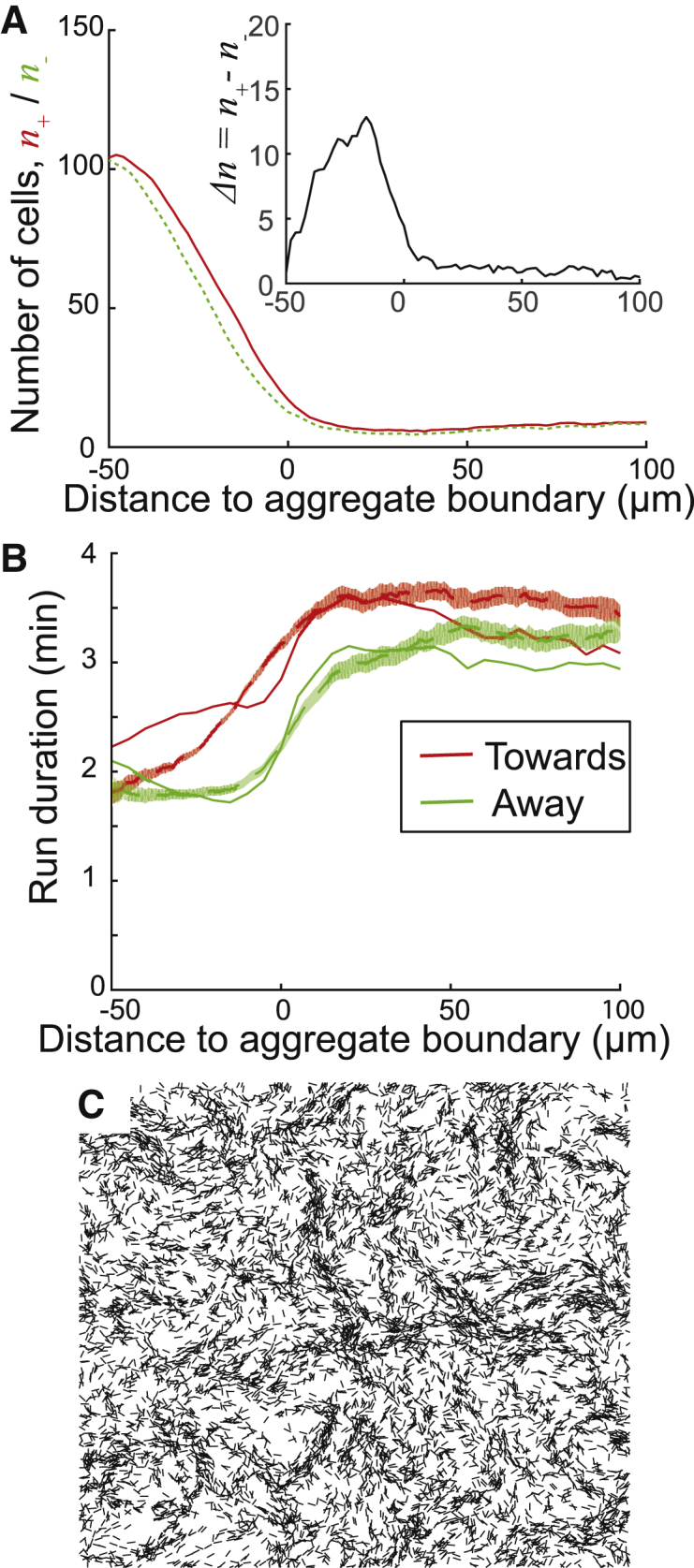
Results of the contact signal model simulations. (A) Agent density (i.e., number of neighbor agents within 3 μm of each agent) around the aggregate in 1D, open-loop simulation as a function of distance to aggregate boundary. The number of agents that move toward the aggregate center (n+) is shown by the red solid line, whereas the number of agents moving away from the aggregate center (n−) is shown by the green dashed line. The inset shows the difference between the two, Δn = n+ − n−. Results are averaged over 23 h time. (B) Experimental run duration data fitted to the proposed contact-signaling model. Red lines indicate run durations of cell moving toward aggregates. Green lines indicate run durations of cells moving away from aggregates. Solid lines are fitted run durations, and dashed lines are experimental results. Red and green shaded areas are bootstrapped 95% confidence intervals calculated from experimental results. Experimental data are from (1). (C) Closed-loop simulation of ABM with contact-dependent signal at 10 h. Run duration of agents is computed using the fitted parameters from (B). Initially, agents are randomly distributed across the simulation domain with a density of 0.3 agent/μm2. As in Fig. 2, the simulation area is 400 × 400 μm, and only 20% of agents are plotted. To see this figure in color, go online.
In our chemotaxis model, we let the probability directly depend on chemotactic signal ρ. We use the following equation to calculate this probability.
| (23) |
Here, ρ is the signal level, and p0, ρ2, and qp are parameters chosen to fit experimental data. Same as above, we did not differentiate cells’ moving direction.
We performed simulations on a 400 × 400 μm area to fit Eq. 23 to mimic the signal produced by an aggregate placed in the center. We let the signal be produced in a circle that is located in the center of the simulation domain with a 50 μm radius. The signal also diffuses and decays with time. We used the steady state of signal level to fit Eq. 23. Because the signal ρ is centrosymmetric, we fit Eq. 23 in one dimension at y = 200 μm.
For nonpersistent state duration, we did not differentiate the moving directions of cells because in this state, cells have very low direct motility. We think the direction during a nonpersistent run is not important.
In the contact-based model, we let the nonpersistent state duration depend on local cell density, ρcell. We use the following equation to fit the mean nonpersistent state duration.
| (24) |
Here, tn is the nonpersistent state duration of cells at low cell density, and cc, ρc2 are parameters to fit the curve. We use the cell density distribution from a 1D, open-loop simulation to fit the experimental data.
In the chemotaxis model, we let the nonpersistent state duration depend on chemotactic signal level ρ. We use the following equation to fit the mean nonpersistent state duration.
| (25) |
Here, tn is the nonpersistent state duration of cells at low chemotactic signal area. qn, ρn, and cn are parameters to fit the curve. We fit the duration in one dimension, using the same signal level used to fit Eq. 23.
The source code of the chemotaxis simulation can be downloaded at https://github.com/zzyustcrice/chemotaxis2.
Results
A phenomenological model matches the patterns of cell alignment
Our recently developed collective-alignment model is based on a biophysically realistic model of flexible M. xanthus cells. The model includes excluded-volume repulsion that prohibits overlap between cells in physical space and also incorporates trail-following behavior (13, 14). This model can explain experimentally observed alignment patterns for wild-type cells and nonreversing mutants at low cell density (0.08 cell/μm2, i.e., the packing fraction is ∼25%) (16). However, the model formalism is too complex to efficiently simulate large numbers of cells. Furthermore, although this model does not allow overlap between cells, at high cell densities, overlap becomes unavoidable. To overcome these shortcomings, we developed a mechanistic ABM that can phenomenologically describe cell alignment dynamics. The model details are given in Materials and Methods and briefly summarized below.
In our ABM, each agent represents a cell as a self-propelled particle on a 2D surface with a center position of (x(t), y(t)) and orientation −π < θ < π. The simulations are conducted on a rectangular 2D area with periodic boundary conditions. At each time step, agents move in the direction of their orientation and turn to align with their neighbors and any trails in the area. No hard-core, excluded-volume repulsion between agents is explicitly modeled (agents are essentially zero volume). However, to avoid biologically unrealistic agent densities, repulsion between agents in a direction perpendicular to their long axis is introduced. To model alignment with neighbors, we used a phenomenological approach based on Sliusarenko et al. (29): each agent changes its orientation to align with neighboring cells at every time step. To model alignment with trails, we used the same approach as in Balagam et al. (13), in which cells turn their long axes to nearby areas with a maximal density of trail matrix.
To compare the phenomenological model with a detailed biophysical model (13), we first simulated reversing and nonreversing agents at low density (0.08 agent/μm2, i.e., ∼25% packing fraction) with our ABM in a 400 × 400 μm domain with periodic boundary conditions and other parameters set according to (13). We found that our model captures the differences in patterns of aligned agent groups (clusters) between reversing and nonreversing agents (Fig. 1). For nonreversing agents, the previous biophysical model (13) shows that agents form isolated clusters (Fig. 1 A). Our model shows a similar pattern (Fig. 1 B). For reversing agents, the previous model (13) shows that agents form an interconnected, mesh-like structure (Fig. 1 C). Our model also shows this pattern for reversing cells (Fig. 1 D). These clustering patterns are also observed in experiments for reversing and nonreversing cells (16). To quantitatively compare the results of the new, to our knowledge, model with the previous biophysical model, we computed the average number of agents in a cluster (defined by a cell density above the threshold; see Fig. S1 caption) as a function of overall agent density (Fig. S1). The two models are in agreement: higher cell densities lead to more agents in a cluster, and trail following is critical for explaining cluster formation for reversing cells. Therefore, our model quantitatively matches the detailed biophysical model but is computationally efficient enough to simulate very high cell densities.
Figure 1.

Comparison of the collective alignment patterns. (A and B) Simulation snapshots of the cell patterns formed by nonreversing agents of the Balagam et al. biophysical model (A) and of our new model (B). (C) An experimental snapshot of the cell patterns of a nonreversing mutant (A+S−Frz−). (D and E) Simulation snapshots of reversing agents of the Balagam et al. model (D) and of our new model (E). (F) An experimental snapshot of alignment patterns of wild-type cells (A+S+Frz+). Experimental pictures are from Fig. 1 of (16), used with permission. For simulations, the area shown is 400 × 400 μm, with an agent density of 0.08 agent/μm2 (packing fraction 0.25). Simulation time is 1 h. For experiments, scale bars, 100 μm.
Cell-density-dependent motility decrease and cell alignment are not sufficient for aggregate formation
Several previously published models of aggregation were based on the hypothesized “traffic-jam mechanism,” in which cells slow down in regions of high density (29, 30). This slowdown further increases local cell density, leading to a positive feedback loop that drives cell aggregation. Cell-tracking experiments by Sliusarenko et al. reported an ∼80% reduction of cell speeds in high-cell-density areas and used these measurements in the model to reproduce aggregation patterns (29). In addition to this slowdown, Sliusarenko et al. postulated that cells sense and align toward a cell-density gradient. The mechanism of such alignment was not explained, and such behavior is unlikely to be realistic unless it emerges from local alignment interactions. Furthermore, subsequent comparison of aggregation dynamics between this traffic-jam model and the experimental results revealed that a traffic jam alone is insufficient to drive aggregation. In particular, although the traffic-jam model can produce aggregates of similar size compared with experiments (30), it fails to display the observed (38) dynamic properties of aggregates such as moving, merging, and splitting, nor does it reproduce the correct time dynamics and extent of aggregation.
Here, to investigate how different mechanisms of cell alignment would affect the aggregation dynamics, we performed multiple simulations of different mechanistic traffic-jam ABMs. Following up on the results of (29), agents reduce their speed by 80% if the local cell density is above 0.6 agent/μm2. Initially, agents are randomly distributed with density 0.3 agent/μm2.
In the first model, we consider no local alignment: all the agents choose random orientations. Running the simulations of this model for 10 h, the natural timescale of aggregation in (1), we observed the emergence of very small aggregates (Fig. 2 A; Video S1). If we continue the simulations for longer times, the aggregation process becomes unrealistically long: even after 50 h, some aggregates are still growing (Fig. S2 A).
Figure 2.

Comparison of the collective behaviors of different models. (A) The traffic-jam model simulation result at 10 h. (B) The traffic-jam model with local alignment simulation result at 10 h. (C) The traffic-jam model with local alignment and trail following simulation result at 10 h. All simulations have agent density 0.3 agent/μm2 and 400 × 400 μm area. To make aggregates more visible, only 20% of randomly selected agents are plotted.
Simulation area is . Initially, agents are randomly distributed across the simulation domain with density 0.3 agent/μm2. Simulation is prerun for 5 hours without chemotactic signal production to align agents. Simulation ends 10 hours after chemotactic signal production. For clarity reason, only 20% of agents are plotted.
In the second model, we also consider local alignment: agents now actively align their long axis with nearby agents. There are more aggregates in Fig. 2 B, and their size is larger than in the simulation in Fig. 2 A. Therefore, in agreement with the results of (2, 29), local alignment helps with aggregation. However, examining the patterns of aggregation dynamics (Fig. S2 B), we note that aggregation is still slower than experimentally observed (1). Moreover, most of the aggregates do not have the circular shape observed in experiments (1, 38), and aggregates do not move, merge, or split.
The results of (3, 13) indicated that trail following further aids aggregation. To test the effect of trail following on the aggregation, we include these effects into our second model. As shown Fig. 2 C, by 10 h, cells converge into streams and form small aggregates at the intersections of streams. However, these aggregates are unusually small and do not grow in size given more simulation time (Fig. S2 C).
From these results, we conclude that a traffic-jam model is not sufficient to form aggregates even when proper alignment mechanisms are included in the model. Moreover, recent results from Cotter et al. showed that cell motility reduction at high cell densities is only ∼60% (1), further impeding the traffic-jam model. Therefore, we can conclude that the motility reduction is insufficient to drive aggregation. This agrees with the conclusion of Cotter et al. (1), who demonstrated that biased walk toward the aggregate center is essential to match experimentally observed aggregation dynamics. However, the biochemical mechanism of the bias has not been identified. In what follows, we test two alternative mechanisms for this biased walk.
The contact-dependent signal model does not lead to stable aggregation. Many previous studies suggest that the reversal frequency is affected by contact with other cells (4, 5, 18, 39, 40). For example, Mauriello et al. demonstrated that when M. xanthus cells make transient side-to-side contact, they exhibit increased cellular reversals (4). Earlier studies also postulated control of reversals during M. xanthus development by cell contact due to C-signal exchange (5, 18, 39, 40). Moreover, mathematical models based on contact-dependent reversal induction successfully reproduce traveling wave patterns formed by M. xanthus cells during development (28). Despite all the work postulating reversal control via C-signal exchange, no molecular mechanism has been identified.
We begin by testing the hypothesis that M. xanthus cells employ a contact-based mechanism to perform a biased walk. To test this hypothesis using our ABM, we assume that an agent’s run duration can be affected by nearby agents’ run directions. If nearby agents are moving in the opposite direction, the target agent will have a shorter run duration. If nearby agents are moving in the same direction, the target agent will have a longer run duration. In this way, when cells form a stream, it is likely that more cells will run in one direction to produce a net flow of cells. When the streams of cells intersect, an aggregate can form at the intersection.
To decide how reversal period is influenced by the direction of nearby cells, we follow the data-driven modeling approaches of Cotter et al. (1). For simplicity, we first run a simple 1D, open-loop simulation, i.e., focus only on cell motility in the radial direction near an aggregate. In this simulation, we assume there is an aggregate in the middle of the simulation domain. This model is completely data driven; agents choose their behaviors from an experimental data set from Cotter et al. (1), which shows cell behaviors at different distances from the aggregate and moving in different directions relative to the aggregate. As in (1), agent behavior is sampled from the recorded data set of cell behaviors conditional on how far the agent is from the aggregate and the agent’s direction relative to the aggregate. To properly account for cellular slowdown inside the aggregates, we follow Cotter et al. (1) to introduce persistent and nonpersistent states into the model. In the persistent state, cells actively move along their long axis, whereas in the nonpersistent state, cells cease movement altogether or jiggle as if pushed by moving cells. These states, and transitions between them, were quantified in the Cotter et al. (1) data set. As a result, decreased cell motility inside aggregates has two components: decreased cell speed in the persistent state compared with cells outside of aggregates and a higher probability of transitioning into a nonpersistent state.
As expected, the biased walk toward aggregates and decreased motility inside aggregates led to agents accumulating in the region of the postulated aggregate. As a result, the density of agents moving toward the aggregates is slightly higher than the density of agents moving away from the aggregates (Fig. 3 A, upper right). Thus, we asked whether the run bias can result from contact-based signaling that relies on an agent sensing nearby agents that move in the same (n+) or opposite (n−) directions. Given the relatively small difference between n+ and n−, we argue that the cell’s reversal period must be sensitive to the sign and the magnitude of the difference in the two. Therefore, we define the signal Δn = n+ − n−. In addition to this signal, the reversal period must also depend on the total cell density ρcell = n+ + n− to ensure a shorter reversal period inside the aggregates regardless of the direction. Therefore, we look for a fit to bias data using
| (26) |
Here, the first term will be a decreasing function of , e.g.,
| (27) |
where τ0 is the mean reversal period at low cell density. Parameters c1, q1, and ρc0 are chosen to fit the experimental data showing more frequent reversals inside the aggregates in which cell density is high. The factor f1 is responsible for the bias in runs, i.e., the difference in reversal periods for cells going toward or away from the aggregates. We use
| (28) |
where c2, q2, and Δn0 are parameters chosen to provide the best fit to experimental data. Using Eqs. 26, 27, and 28, we can fit the reversal period bias (Fig. 3 B). From the results, we can conclude that within the framework of this open-loop, 1D model, this contact-signal mechanism can approximate the run duration data acquired from experiments. To test whether the small deviation between the observed and fitted reversal period bias in Fig. 3 B does not hinder aggregation, we ran a data-driven, open-loop simulation using fitted bias data. In the same fashion, we assume that the aggregate is in the middle of the simulation domain, and agent behaviors are sampled from the experimental data sets, except for run duration data, which are sampled from the fitted data. Fig. S3 A demonstrated that aggregation proceeds in a similar fashion. However, it is not clear whether this mechanism will work in the more rigorous 2D, closed-loop model.
To investigate whether contact-dependent reversal period modulation will aid aggregation, we performed 2D simulations using the model with the directional sensing mechanism. In two dimensions, we use cell orientation angle θ to decide whether two cells are moving in the same direction or the opposite direction: if cell i and cell j satisfy cos(θi − θj) > 0, we assume that cell i and cell j are moving in the same direction; otherwise, the opposite direction. In this model, each agent’s reversal period is given by Eqs. 26, 27, and 28, and the probability of transitioning to a nonpersistent state is dependent on local agent density. In Fig. 3 C, we see that after 10 h of simulation, this model does not produce any aggregates. Moreover, no stable aggregates form even at longer simulation times (Fig. S3 C). In addition, we added this contact signal into the traffic-jam model in Fig. 2 C and compared the aggregation behaviors (Fig. S3 B). The results show that the contact signal improves aggregation somewhat, but the aggregation rate is still much slower than the experiments. Therefore, we conclude that the contact-based signal mechanism is not sufficient for aggregation, and an alternative mechanism for the biased walk of M. xanthus cells is needed.
A chemotaxis model produces biased movement similar to that observed in experiments and improves aggregation
Previous experiments have shown that M. xanthus cells can move up a gradient of lipid extracted from starving cells by increasing their reversal period (6). At any given concentration, the increase is temporary because cells eventually adapt to the chemotactic signal (6). This process is dependent on chemosensory systems similar to those found in other bacteria (7). We propose that the movement bias during aggregation is caused by chemotaxis toward a chemotactic signal produced by cells. In our model, a large number of cells in an aggregate produce a concentration gradient of a chemotactic signal that deceases with distance from the aggregate. Cells outside the aggregate are then attracted to the aggregate though a biased walk typical of bacterial chemotaxis systems (41).
Based on previous models of chemotaxis with adaptation (8, 9, 10), we developed our phenomenological model using integral feedback control (Fig. 4 A; see Materials and Methods for details). We let agents produce and detect a signaling molecule (concentration denoted as ρ in Fig. 4 A), which diffuses and decays with time. At the high cell densities inside aggregates, a gradient of ρ surrounding the aggregate can bias cell movement toward aggregation centers. Signal ρ excites an internal signal of the agents y1, which corresponds to the activation of receptors in cells. y2 is the integral of y1 and feeds back to the system to inhibit y1 and deactivate the chemoreceptors (e.g., via demethylation). Therefore, y1 and y2 form an integral feedback loop for adaptation. Next, we let the reversal period depend on y1 and y2:
| (29) |
where F, G: R → (0, ∞). Based on the experimental data (1), agents have shorter run durations inside aggregates. Because inside aggregates, the signal ρ is higher, the steady state of y2 is also larger for agents inside aggregates than agents outside aggregates. Therefore, G decreases as a function of y2. For F(y1), when agents move up the chemotactic signal gradient, ρ increases, and the excitation from ρ is stronger than the inhibition, y1 > 0. Similarly, when agents move down the chemotactic signal gradient aggregates, y1 < 0. Therefore, to make agents bias to longer reversal times as they move up the chemotactic signal gradient, F needs to be increasing as a function of y1. Note that given that y1 is proportional to the time derivative of y2, we can interpret Eq. 29 as the reversal period decreasing as a function of signal but increasing as a function of time derivative of a signal. As a result, agents moving up the gradient of signal will increase their run periods. Thus, the implemented chemotaxis model with adaptation is the simplest mechanistic way to enable agents to distinguish between going into and out of aggregates.
Figure 4.

Results of a chemotaxis model. (A) The adaptation network with an integral feedback loop used in our chemotaxis model. (B) An example of a chemotactic signal distribution. The chemotactic signal is produced in a circle in the center with fixed decay and diffusion rates. Upper right inset shows chemotactic signal in the simulation region at steady state. The main panel shows chemotactic signal as a function of distance to aggregate center at steady state. The dashed line marks the boundary of the assumed aggregate. (C) A comparison of run duration biases produced by simulation (solid lines) and experimental data (dashed lines). Red lines (black lines in grayscale figure) are runs pointing toward the aggregate centroid, whereas green lines (gray lines in grayscale figure) are runs pointed away from the aggregate centroid. Shaded areas are bootstrapped 95% confidence intervals of experiment data. (D) Aggregate size distribution in multiple simulations. Blue is simulations of fixed chemotactic signal production rate, and black is simulations of chemotactic signal production with positive feedback. (E) Simulation of the chemotaxis model. Run duration is acquired from the fitted duration in (C). (F) Same as (E), plus positive feedback in signal production. Initially, agents are randomly distributed across the simulation domain with density 0.3 agent/μm2. ABMs are run for 5 h without chemotaxis so that agents become aligned. The snapshot is taken after 10 h of simulation with chemotaxis. The simulation area is 400 × 400 μm, and only 20% of agents are plotted. To see this figure in color, go online.
Considering F, G > 0 for all possible inputs, we chose
| (30) |
where a, b are chosen to fit the experiment data. We note that the exponential form of the function is phenomenological but should not matter as long as a reasonable fit to the experimental data set is obtained, as in Fig. 3 C. To model slowdown of cells in high-density areas as with the experimental data (1), we make agents switch to a nonpersistent motility state with the rate dependent on ρ (see Materials and Methods for details).
The gradient profile around the aggregate is determined by the diffusion and degradation of the signaling molecule. We use the diffusion coefficient of lipids (37) and fit the value of the degradation constant to match the range of bias around the aggregates. To determine values for the parameters in our model that match the bias observed in (1), we performed several 2D simulations. In each simulation, the chemotactic signal is produced in a circle at the center of the simulation domain assumed to be an aggregate. The sizes of the circle are different in each simulation and are determined by the distribution of aggregates measured in experiments (1). Fig. 4 B shows a chemotactic signal profile produced in one of these simulations. To measure the biased walk of agents, we average the run durations based on run direction and distance to aggregate boundary for all simulations. The results in Fig. 4 C show that this mechanism produces bias that matches the experimental observations.
To investigate whether the chemotaxis model aids aggregation, we performed 2D simulations using the mechanistic ABM with chemotaxis. Following the approaches of (1), agents were allowed to align before the onset of aggregation, i.e., ABM simulations were run for 5 h with the terms responsible for producing the chemotactic signal set to 0. After 5 h alignment, agents begin to produce the chemotactic signal and perform biased movement. After 10 h of chemotaxis simulation, agents form aggregates with clear boundaries (Fig. 4 E). However, we note that the average size of the aggregates in such simulations (mean area ≈ 4000 μm2) is somewhat smaller than those in the experiment (mean area ≈ 6000 μm2). Moreover, the run durations computed from closed-loop simulations did not quite match the experimental data (Fig. S4 A). To correct this issue, we increased agent bias toward larger aggregates with positive feedback in chemotactic signal production: agents produce more chemotactic signal when in an environment with high signal concentration (see Materials and Methods for detailed implementation). We find that this positive feedback in signal production can produce larger aggregates (Fig. 4, D and F) and further matches the experimentally observed trends (Fig. S4 B). Thus, we conclude that this chemotaxis model can produce biased movement and stable aggregates. We then performed larger-scale simulations that quantitatively compare the results of this model with the experimental observations of Cotter et al. (1).
A chemotaxis model qualitatively reproduces cell alignment patterns
One of the most unexpected results of Cotter et al. (1) was a finding that M. xanthus cells away from aggregates align their moving direction in a radial direction with respect to the nearest aggregate and that the alignment aids aggregation. On the other hand, cells inside aggregates and near the aggregate boundary align in the tangential direction, i.e., rotate around the aggregate (1). To see if our mechanistic ABM with alignment, trail following, and chemotaxis can reproduce this alignment pattern, we performed simulations using the chemotaxis model described in last section. Because the microscope field of view in the experiment is 986 × 740 μm, we increased our simulation domain to 1 × 1 mm to better compare with the experiment.
First, we compared the alignment patterns of our model and experiment (Fig. 5, A–D). We follow the definitions of Cotter et al. (1) and for each agent define a run vector that corresponds to the agent’s displacement between changes in agent’s state, i.e., between reversals and/or switching to between persistent state. Alignment of agent runs to aggregate centroids is quantified by measuring the alignment coefficient, defined as an average value of , where is the direction of a run vector i and is the angle of a vector pointing from the position at the beginning of the run to the centroid of the nearest aggregate. Averaging is done over all agent runs in the simulation. Negative alignment coefficient to aggregates indicates that agents are aligned tangentially, i.e., rotating around the aggregate; positive alignment coefficient indicates that agents are aligned radially relative to the aggregate. Our results (Fig. 5 A) show that in agreement with the experimental observations of Cotter et al (1), alignment coefficient is negative near aggregate boundaries but is positive further away from the aggregates. This result shows that our model is sufficient to explain cell alignment within and around aggregates. To further compare observed and simulated orientation pattern dynamics, we quantified alignment coefficient at different times in the simulation (Fig. 5 C). The results indicate that the alignment coefficient near aggregate boundaries decreases with time, i.e., making the tangential orientation of agents more pronounced. Thus, as the aggregates grow, there are more cells near the boundary circulating around the center, and the alignment coefficient becomes more negative as time increases. We test this prediction by reprocessing the data from Cotter et al. (1) in different time windows. The results demonstrate the same trend as predicted in the model (Fig. 5 D). Furthermore, we show (Fig. 5 B) comparable values in experiment and simulation in the local alignment coefficient defined (1) as an average value of cos(2(θi − θj)) over all runs i and j that started within certain time and distance from one another. We note that in our simulations, the local alignment of cells is slightly weaker than the experiment, and perhaps more parameter fitting is needed for quantitative agreement.
Figure 5.

Comparison between simulation and experimental results. The simulation area is 1 × 1 mm. The simulation is prerun for 5 h without chemotactic signal production to align agents. (A) The alignment strength of run vectors with vector pointing toward nearest aggregate centroid. The red line (gray line in grayscale figure) is the experimental result, the solid line is the mean, and the dashed line marks the 95% confidence intervals. The black line is the simulation result. Negative distances indicate that the run began inside an aggregate. Values may span (−1, 1), where 1 indicates vectors are parallel. Likewise, −1 indicates vectors are perpendicular. (B) The run vector alignment strength with neighboring run vectors that occurred within ±5 min and 15 μm of different run durations. Values may span (−1, 1) as in (A). (C) The alignment strength of run vectors with vector pointing toward nearest aggregate centroid at different times in simulation. Results are averaged for run vectors within a 1 h time window. (D) The alignment strength of run vectors with vector pointing toward nearest aggregate centroid at different times in experiment. Results are averaged for run vectors within the 1 h time window. (E) The fraction of cells in aggregate in experiment (red) and simulation (black). (F) Aggregate size distribution at 5 h in experiment (red) and at 8 h in simulation (black). The measurement time point in simulation is chosen when the fraction of cells inside aggregate reaches 60%. The aggregate size distribution is measured for multiple simulations with more than 100 aggregates. To see this figure in color, go online.
Comparison of aggregation dynamics in our model to the experimental observations in (1) indicates similar aggregation rates. (Fig. 5 E). We note that the quantitative agreement between the model and the experiments can be further improved by the offset between the time point of 0 h between the two. We assumed that in the model, t = 0 h is the time when agents start chemotactic signal production. In the experiment, the timing is set by the imaging protocol, and we do not know when the chemotaxis starts. Nonetheless, the rate of aggregation in simulations is a bit slower: it takes ∼8 h for the fraction of cells inside aggregates to reach ∼60%, as compared to 5 h in the experiments. However, continuing the simulation for longer, we observe that by 10 h, over 65% of the agents will end up in the aggregates. The distribution of aggregate sizes (Fig. 5 F) further demonstrates quantitative agreement between the simulations (black bars) and experiments of (1) (red bars). However, the agreement is not perfect because the model produces slightly more large aggregates over 5000 μm2 and fewer small aggregates below 5000 μm2. This agreement may be improved by further tuning the positive feedback in the chemotactic signal production but is beyond the scope of this work. Nevertheless, the model shows remarkable agreement with most of the features of aggregation dynamics quantified by Cotter et al. (1).
Discussion
In this work, we developed a mechanistic ABM that matches many dynamic features observed during aggregation and provides plausible mechanistic explanations for these cell behaviors (1). Given the importance of cell alignment in aggregation, we started by developing a phenomenological framework that approximates interactions of the previous biophysical model (13). The framework can reproduce the different cell alignment behaviors of reversing and nonreversing M. xanthus cells at low cell densities (16) and can be scaled to much higher aggregation cell densities with multiple cell layers. Next, we explored possible mechanisms of the biased walk toward the aggregates (1). We showed that a chemotaxis model, but not a contact-based signal model, produces stable aggregates and the biased movement in our model. Remarkably, the resulting model also matches the experimentally observed cell alignment patterns.
Why would the chemotaxis but not the contact-signaling model reproduce aggregation patterns? We argue that the failure of a contact-based signal model to produce stable aggregates is due to its high sensitivity to noise. As seen in Fig. 3 A, differences between the densities of cells going toward versus away from the aggregates are much smaller in comparison with the local cell density. Therefore, when this difference is used as an input signal biasing cell reversal, the fluctuations in local cell density could significantly affect its value. On the other hand, the production of chemoattractant is directly proportional to the total cell density, but its concentration changes gradually over time. The ability of cells to detect both the value and time derivative (via adaptive network) of the signal allows cells time to aggregate in high chemotactic signal areas.
We note that the question of whether chemotaxis is required for formation of stable aggregates in M. xanthus has been subject to numerous prior investigations (42, 43, 44). Depending on the implementation mechanisms, contact-based chemokinesis may or may not be sufficient to form aggregates. Notably, these studies did not constrain the parameters of the signaling mechanism with experimental measurements of cellular behaviors and did not compare the dynamics of aggregate growth in the models with the experiments. In our work, we demonstrate that only chemotaxis-based signaling mechanisms are compatible with the constraints imposed by the data set of Cotter et al. (1).
Our simulations match the observations from Cotter et al. (1) that away from the aggregate boundaries, cells tend to align radially to aggregate centers (Fig. 5 A), whereas closer to the aggregate boundaries, tangential (circumferential) orientation patterns are observed (Fig. 5 A). We note that in the model, the orientation of agents is not directly affected by aggregate positions or agent density or chemotactic signal gradients. Therefore, our model predicts that the observed alignment patterns are the result of the two major factors affecting collective cellular alignment dynamics: alignment to nearby cells and to the secreted trails. As a result of these factors, cells align and form streams before the initiation of aggregation. Once aggregation initiates, cells predominately move along the streams, and as a result, aggregates tend to form in the regions where these streams intersect. Because cells tend to move toward aggregates, aggregate size and cell density inside aggregates increase. At the high cell densities that exist inside an aggregate, cells may not be able to move any closer to the aggregate center (because of local repulsion) but instead start moving in the tangential direction. Further away from the aggregates, cells continue to move along the streams toward or away from the aggregate, which leads to radial orientation patterns with respect to aggregates. The radial orientation patterns become weaker as the density of cells outside the aggregate decreases.
Although we focused mainly on qualitative agreement between our model and experimental aggregation patterns, we nevertheless achieved quantitative agreement with multiple aggregate properties. We believe that this agreement can be further improved in future work because our models ignore certain aspects of cell behaviors observed by Cotter et al. (1). For example, the amount of stochasticity in the individual cell behaviors will undoubtedly affect the aggregation dynamics. The results of Cotter et al. showed wide variation in the persistent run durations of cells (1). In our simulations, we set the noise to be somewhat smaller and did not investigate its effect on aggregation. Investigating the effect of noise on aggregation will be an interesting direction for future work. Furthermore, during our aggregation simulations, we assumed time-independent cell behavior, but the results of Cotter et al. showed dynamical changes in cell speed and run durations. The effect of this variability will also be systematically investigated in future studies. Notably, the cells display longer reversal periods in the beginning of aggregation (1), and long reversal periods combined with steric interactions and trail following have been shown (13) to enable formation of circular aggregates—cell streams that close on themselves. It remains to be seen if these aggregates can serve as nucleation centers for mature aggregates. Nevertheless, our model makes important predictions about the cellular interactions that drive multicellular aggregation and can serve as a basis to investigate a wider range of developmental mutant strains.
Author Contributions
Designed research, Z.Z. and O.A.I.; performed research, Z.Z.; analyzed data, Z.Z., contributed analytic tools, C.C.; wrote the manuscript, Z.Z., C.C., L.J.S., and O.A.I.
Acknowledgments
The research reported here was supported by the National Science Foundation under awards PHY-1427654 (for Center for Theoretical Biological Physics), MCB-1411780 (to O.A.I.), and MCB-1411891 (to L.J.S.).
Editor: Ruth Baker.
Footnotes
Six figures, one table, and one video are available at http://www.biophysj.org/biophysj/supplemental/S0006-3495(18)31226-8.
Supporting Material
References
- 1.Cotter C.R., Schüttler H.B., Shimkets L.J. Data-driven modeling reveals cell behaviors controlling self-organization during Myxococcus xanthus development. Proc. Natl. Acad. Sci. USA. 2017;114:E4592–E4601. doi: 10.1073/pnas.1620981114. [DOI] [PMC free article] [PubMed] [Google Scholar]
- 2.Kiskowski M.A., Jiang Y., Alber M.S. Role of streams in myxobacteria aggregate formation. Phys. Biol. 2004;1:173–183. doi: 10.1088/1478-3967/1/3/005. [DOI] [PubMed] [Google Scholar]
- 3.Stevens A. A stochastic cellular automaton modeling gliding and aggregation of myxobacteria. SIAM J. Appl. Math. 2000;61:172–182. [Google Scholar]
- 4.Mauriello E.M., Astling D.P., Zusman D.R. Localization of a bacterial cytoplasmic receptor is dynamic and changes with cell-cell contacts. Proc. Natl. Acad. Sci. USA. 2009;106:4852–4857. doi: 10.1073/pnas.0810583106. [DOI] [PMC free article] [PubMed] [Google Scholar]
- 5.Sliusarenko O., Neu J., Oster G. Accordion waves in Myxococcus xanthus. Proc. Natl. Acad. Sci. USA. 2006;103:1534–1539. doi: 10.1073/pnas.0507720103. [DOI] [PMC free article] [PubMed] [Google Scholar]
- 6.Kearns D.B., Shimkets L.J. Chemotaxis in a gliding bacterium. Proc. Natl. Acad. Sci. USA. 1998;95:11957–11962. doi: 10.1073/pnas.95.20.11957. [DOI] [PMC free article] [PubMed] [Google Scholar]
- 7.Xu Q., Black W.P., Yang Z. Independence and interdependence of Dif and Frz chemosensory pathways in Myxococcus xanthus chemotaxis. Mol. Microbiol. 2008;69:714–723. doi: 10.1111/j.1365-2958.2008.06322.x. [DOI] [PMC free article] [PubMed] [Google Scholar]
- 8.Erban R., Othmer H.G. From individual to collective behavior in bacterial chemotaxis. SIAM J. Appl. Math. 2004;65:361–391. [Google Scholar]
- 9.Barkai N., Leibler S. Robustness in simple biochemical networks. Nature. 1997;387:913–917. doi: 10.1038/43199. [DOI] [PubMed] [Google Scholar]
- 10.Kollmann M., Løvdok L., Sourjik V. Design principles of a bacterial signalling network. Nature. 2005;438:504–507. doi: 10.1038/nature04228. [DOI] [PubMed] [Google Scholar]
- 11.Csahók Z., Vicsek T. Lattice-gas model for collective biological motion. Phys. Rev. E Stat. Phys. Plasmas Fluids Relat. Interdiscip. Topics. 1995;52:5297–5303. doi: 10.1103/physreve.52.5297. [DOI] [PubMed] [Google Scholar]
- 12.Kim S.K., Kaiser D. Cell alignment required in differentiation of Myxococcus xanthus. Science. 1990;249:926–928. doi: 10.1126/science.2118274. [DOI] [PubMed] [Google Scholar]
- 13.Balagam R., Igoshin O.A. Mechanism for collective cell alignment in Myxococcus xanthus bacteria. PLoS Comput. Biol. 2015;11:e1004474. doi: 10.1371/journal.pcbi.1004474. [DOI] [PMC free article] [PubMed] [Google Scholar]
- 14.Balagam R., Litwin D.B., Igoshin O.A. Myxococcus xanthus gliding motors are elastically coupled to the substrate as predicted by the focal adhesion model of gliding motility. PLoS Comput. Biol. 2014;10:e1003619. doi: 10.1371/journal.pcbi.1003619. [DOI] [PMC free article] [PubMed] [Google Scholar]
- 15.Spormann A.M. Gliding motility in bacteria: insights from studies of Myxococcus xanthus. Microbiol. Mol. Biol. Rev. 1999;63:621–641. doi: 10.1128/mmbr.63.3.621-641.1999. [DOI] [PMC free article] [PubMed] [Google Scholar]
- 16.Starruß J., Peruani F., Bär M. Pattern-formation mechanisms in motility mutants of Myxococcus xanthus. Interface Focus. 2012;2:774–785. doi: 10.1098/rsfs.2012.0034. [DOI] [PMC free article] [PubMed] [Google Scholar]
- 17.Wall D., Kaiser D. Alignment enhances the cell-to-cell transfer of pilus phenotype. Proc. Natl. Acad. Sci. USA. 1998;95:3054–3058. doi: 10.1073/pnas.95.6.3054. [DOI] [PMC free article] [PubMed] [Google Scholar]
- 18.Welch R., Kaiser D. Cell behavior in traveling wave patterns of myxobacteria. Proc. Natl. Acad. Sci. USA. 2001;98:14907–14912. doi: 10.1073/pnas.261574598. [DOI] [PMC free article] [PubMed] [Google Scholar]
- 19.Pelling A.E., Li Y., Gimzewski J.K. Self-organized and highly ordered domain structures within swarms of Myxococcus xanthus. Cell Motil. Cytoskeleton. 2006;63:141–148. doi: 10.1002/cm.20112. [DOI] [PubMed] [Google Scholar]
- 20.Li Y., Sun H., Shi W. Extracellular polysaccharides mediate pilus retraction during social motility of Myxococcus xanthus. Proc. Natl. Acad. Sci. USA. 2003;100:5443–5448. doi: 10.1073/pnas.0836639100. [DOI] [PMC free article] [PubMed] [Google Scholar]
- 21.Kearns D.B., Venot A., Shimkets L.J. Identification of a developmental chemoattractant in Myxococcus xanthus through metabolic engineering. Proc. Natl. Acad. Sci. USA. 2001;98:13990–13994. doi: 10.1073/pnas.251484598. [DOI] [PMC free article] [PubMed] [Google Scholar]
- 22.Bonner P.J., Shimkets L.J. Phospholipid directed motility of surface-motile bacteria. Mol. Microbiol. 2006;61:1101–1109. doi: 10.1111/j.1365-2958.2006.05314.x. [DOI] [PubMed] [Google Scholar]
- 23.Wu Y., Jiang Y., Alber M. Social interactions in myxobacterial swarming. PLoS Comput. Biol. 2007;3:e253. doi: 10.1371/journal.pcbi.0030253. [DOI] [PMC free article] [PubMed] [Google Scholar]
- 24.Velicer G.J., Yu Y.T. Evolution of novel cooperative swarming in the bacterium Myxococcus xanthus. Nature. 2003;425:75–78. doi: 10.1038/nature01908. [DOI] [PubMed] [Google Scholar]
- 25.Xiao Y., Wei X., Wall D. Antibiotic production by myxobacteria plays a role in predation. J. Bacteriol. 2011;193:4626–4633. doi: 10.1128/JB.05052-11. [DOI] [PMC free article] [PubMed] [Google Scholar]
- 26.Pérez J., Muñoz-Dorado J., Santamaría R.I. Myxococcus xanthus induces actinorhodin overproduction and aerial mycelium formation by Streptomyces coelicolor. Microb. Biotechnol. 2011;4:175–183. doi: 10.1111/j.1751-7915.2010.00208.x. [DOI] [PMC free article] [PubMed] [Google Scholar]
- 27.Igoshin O.A., Goldbeter A., Oster G. A biochemical oscillator explains several aspects of Myxococcus xanthus behavior during development. Proc. Natl. Acad. Sci. USA. 2004;101:15760–15765. doi: 10.1073/pnas.0407111101. [DOI] [PMC free article] [PubMed] [Google Scholar]
- 28.Zhang H., Vaksman Z., Igoshin O.A. The mechanistic basis of Myxococcus xanthus rippling behavior and its physiological role during predation. PLoS Comput. Biol. 2012;8:e1002715. doi: 10.1371/journal.pcbi.1002715. [DOI] [PMC free article] [PubMed] [Google Scholar]
- 29.Sliusarenko O., Zusman D.R., Oster G. Aggregation during fruiting body formation in Myxococcus xanthus is driven by reducing cell movement. J. Bacteriol. 2007;189:611–619. doi: 10.1128/JB.01206-06. [DOI] [PMC free article] [PubMed] [Google Scholar]
- 30.Zhang H., Angus S., Welch R.D. Quantifying aggregation dynamics during Myxococcus xanthus development. J. Bacteriol. 2011;193:5164–5170. doi: 10.1128/JB.05188-11. [DOI] [PMC free article] [PubMed] [Google Scholar]
- 31.Burchard R.P. Trail following by gliding bacteria. J. Bacteriol. 1982;152:495–501. doi: 10.1128/jb.152.1.495-501.1982. [DOI] [PMC free article] [PubMed] [Google Scholar]
- 32.Berleman J.E., Zemla M., Auer M. Exopolysaccharide microchannels direct bacterial motility and organize multicellular behavior. ISME J. 2016;10:2620–2632. doi: 10.1038/ismej.2016.60. [DOI] [PMC free article] [PubMed] [Google Scholar]
- 33.Zusman D.R., Scott A.E., Kirby J.R. Chemosensory pathways, motility and development in Myxococcus xanthus. Nat. Rev. Microbiol. 2007;5:862–872. doi: 10.1038/nrmicro1770. [DOI] [PubMed] [Google Scholar]
- 34.Großmann R., Peruani F., Bär M. Diffusion properties of active particles with directional reversal. New J. Phys. 2016;18:043009. [Google Scholar]
- 35.Yi T.M., Huang Y., Doyle J. Robust perfect adaptation in bacterial chemotaxis through integral feedback control. Proc. Natl. Acad. Sci. USA. 2000;97:4649–4653. doi: 10.1073/pnas.97.9.4649. [DOI] [PMC free article] [PubMed] [Google Scholar]
- 36.Rao S.S. Prentice Hall Professional Technical Reference; Upper Saddle River, NJ: 2001. Applied Numerical Methods for Engineers and Scientists. [Google Scholar]
- 37.Kearns D.B., Shimkets L.J. Directed movement and surface-borne motility of Myxococcus and Pseudomonas. Methods Enzymol. 2001;336:94–102. doi: 10.1016/s0076-6879(01)36582-5. [DOI] [PubMed] [Google Scholar]
- 38.Xie C., Zhang H., Igoshin O.A. Statistical image analysis reveals features affecting fates of Myxococcus xanthus developmental aggregates. Proc. Natl. Acad. Sci. USA. 2011;108:5915–5920. doi: 10.1073/pnas.1018383108. [DOI] [PMC free article] [PubMed] [Google Scholar]
- 39.Igoshin O.A., Mogilner A., Oster G. Pattern formation and traveling waves in myxobacteria: theory and modeling. Proc. Natl. Acad. Sci. USA. 2001;98:14913–14918. doi: 10.1073/pnas.221579598. [DOI] [PMC free article] [PubMed] [Google Scholar]
- 40.Igoshin O.A., Neu J., Oster G. Developmental waves in myxobacteria: a distinctive pattern formation mechanism. Phys. Rev. E Stat. Nonlin. Soft Matter Phys. 2004;70:041911. doi: 10.1103/PhysRevE.70.041911. [DOI] [PubMed] [Google Scholar]
- 41.Macnab R.M., Koshland D.E., Jr. The gradient-sensing mechanism in bacterial chemotaxis. Proc. Natl. Acad. Sci. USA. 1972;69:2509–2512. doi: 10.1073/pnas.69.9.2509. [DOI] [PMC free article] [PubMed] [Google Scholar]
- 42.Stevens A., Othmer H.G. Aggregation, blowup, and collapse: the ABC’s of taxis in reinforced random walks. SIAM J. Appl. Math. 1997;57:1044–1081. [Google Scholar]
- 43.D’Orsogna M.R., Suchard M.A., Chou T. Interplay of chemotaxis and chemokinesis mechanisms in bacterial dynamics. Phys. Rev. E Stat. Nonlin. Soft Matter Phys. 2003;68:021925. doi: 10.1103/PhysRevE.68.021925. [DOI] [PubMed] [Google Scholar]
- 44.Sozinova O., Jiang Y., Alber M. A three-dimensional model of myxobacterial aggregation by contact-mediated interactions. Proc. Natl. Acad. Sci. USA. 2005;102:11308–11312. doi: 10.1073/pnas.0504259102. [DOI] [PMC free article] [PubMed] [Google Scholar]
Associated Data
This section collects any data citations, data availability statements, or supplementary materials included in this article.
Supplementary Materials
Simulation area is . Initially, agents are randomly distributed across the simulation domain with density 0.3 agent/μm2. Simulation is prerun for 5 hours without chemotactic signal production to align agents. Simulation ends 10 hours after chemotactic signal production. For clarity reason, only 20% of agents are plotted.