Linear and Differential Ion Mobility Separations of Middle-Down Proteoforms

Abstract

Comprehensive characterization of proteomes comprising the same proteins with distinct post-translational modifications (PTMs) is a staggering challenge. Many such proteoforms are isomers (localization variants) that require separation followed by top-down or middle-down mass-spectrometric analyses, but condensed-phase separations are ineffective in those size ranges. The variants for “middle-down” peptides were resolved by differential ion mobility spectrometry (FAIMS) relying on the mobility increment at high electric fields, but not previously by linear IMS based on absolute mobility. We now use complete histone tails with diverse PTMs on alternative sites to demonstrate that high-resolution linear IMS, here trapped IMS (TIMS), broadly resolves the variants of ~50 residues fully or into binary mixtures quantifiable by tandem MS, largely thanks to orthogonal separations across charge states. Separations using traveling-wave (TWIMS) and/or involving various timescales and electrospray ionization source conditions are similar (with lower resolution for TWIMS), showing the transferability of results across linear IMS instruments. The linear IMS and FAIMS dimensions are substantially orthogonal, suggesting FAIMS/IMS/MS as a powerful platform for proteoform analyses.

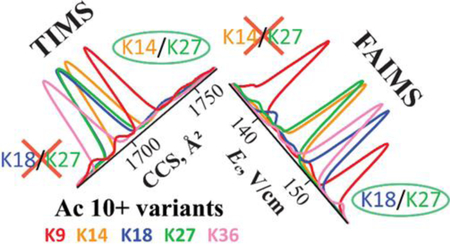
Graphical Abstract

As the proteomics tools mature, the front line moves to characterizing proteoforms and revealing the activity-modulating impacts of post-translational modifications (PTMs).^1–5 Many proteoforms feature different numbers or type of PTMs, detectable by mass spectrometry (MS) on the basis of the mass increment.⁶ Others are isomers with identical PTMs on different residues.^7–9 Such “localization variants” are individually distinguishable by unique fragments in tandem MS, particularly employing electron transfer dissociation (ETD) that severs the protein backbone while retaining weaker PTM links.^3,7,9–11 The conundrum is that multiple variants frequently coexist in cells, but MS/MS cannot disentangle mixtures of more than two, as those with PTMs on internal sites yield no unique fragments.^12,13 This calls for variant separation at least to binary mixtures before the MS/MS step.^12–14 Liquid chromatography (LC) could resolve some variants for peptides in the “bottom-up” mass range (<2.5 kDa) usual for tryptic digests,¹⁵ but not “middle-down” peptides (2.5 – 10 kDa) or intact proteins. Unfortunately, splitting proteins into peptides using proteases precludes global PTM mapping by obliterating the proteoform-specific connectivity information between the modified peptides.^9,16

This problem is most prominent for histones that combine exceptional importance to life with great diversity of PTM types and sites.^9,16–26 Histones (H2A, H2B, H3, and H4) consisting of ~100 – 140 residues are nucleosome core particles - the spools that store the DNA in cell nuclei and regulate chromatin structure and function through dynamic reversible PTMs including methylation (me), trimethylation (me3), acetylation (ac), phosphorylation (p), and others.^9,14,16–26 Permuting their order and modulating the site occupation levels in this “histone code” drastically alters the activity of the whole genome, defined chromatin domains, genomic regions, and/or individual genes. Nearly all PTMs in histones are on the enzymatically cleavable N-terminal domains (“tails”) protruding from the nucleosome.^16,24-²⁵ The H3 tail of ~50 residues is cleavable by the endoproteinase Glu-C, and its characterization approaches that of intact histone.^23–25

A growing alternative to LC is ion mobility spectrometry (IMS), which is based on the ion transport in gases driven by an electric field,^27,28 with key benefits of speed and distinct (often superior) selectivity. Linear IMS²⁷ measures the absolute ion mobility (K) at low field strength (E), whereas differential or field asymmetric waveform IMS (FAIMS)²⁸ relies on the difference between K at high and low E elicited by an asymmetric waveform. That ΔK is less correlated^29,30 to the ion mass (m) than K, rendering FAIMS more orthogonal to MS than linear IMS is - by about 4-fold for many biomolecular classes comprising peptides.^31,32 Therefore, FAIMS commonly separates isomers better than linear IMS of the same resolving power (R), including peptides with sequence inversions³² and localization variants with diverse PTMs.^14,33–37 In particular, complete histone tails and their segments involving various PTMs and sites have been resolved.^14,34,35

Linear IMS separations of such variants were limited to phosphopeptides under −1.5 kDa.^38,39 Expanding this capability to larger peptides and smaller PTMs is topical, as linear IMS platforms can be more sensitive than high-definition FAIMS. They also determine the collision cross section (Ω) unavailable from FAIMS,^27,28 which may help under-standing and predicting the PTM-controlled differences in stability of peptide folds with implications for activity in vivo.⁴⁰ Here we deploy linear IMS in the commercial traveling wave (TWIMS)^41–47 and trapped (TIMS)^48–53 platforms to separate localization variants for complete histone tails. The instrumental resolving power of TIMS can exceed 300, far over ~50 with TWIMS.^42,53,54 However, R for proteins in linear IMS has been capped at ~30 by peak broadening due to conformational multiplicity.^55,56 A critical advantage of TIMS is achieving for some protein conformers same peak width as for small peptides, as in FAIMS.^52,57

We utilize the H3 variants investigated¹⁴ by FAIMS to compare performance and evaluate the orthogonality between two dimensions for middle-down proteoforms. We also inspect the correlation between TWIMS and TIMS to gauge the transferability across linear IMS platforms.

Experimental Methods

We probed the 18 H3.1 tails (residues 2 – 51, monoisotopic mass 5,350 Da) with PTMs (me, me3, ac, and p) in biologically relevant positions (Table 1).¹⁴ These were fused by native chemical ligation⁵⁸ from two 25-residue peptides assembled by solid-state synthesis involving modified amino acids.¹⁴ Protonated peptides were generated by electrospray ionization (ESI). The IMS/MS spectra were acquired for each species individually, with separations verified using equimolar mixtures of two or more variants.

Table 1.

Sequence of H3 tail and PTM localizations

Sequence	PTM	Positions
ART3K4QT6ARK9S10 TGGK14APRK18QL ATK23AARK27S28AP ATGGVK36KPHR Y41RPGTVALRE	me	K4, K9, K23
	me3	K4, K9, K23, K27, K36
	ac	K9, K14, K18, K27, K36
	p	T3, T6, S10, S28, Y41

ESI-TWIMS-MS Instrumentation.

In TWIMS,^41–47 ions “surf’ along a stack of addressable electrodes that create an axial wave with spatial period L and radially confining rf field. We employed the Synapt G2 system (Waters, Milford, MA), where exiting ions are injected into an orthogonal reflectron time-of-flight (ToF) stage (resolving power Rms of 20,000) and registered.⁴² As isobaric ions have the same velocity under vacuum, their temporal separation at the detector equals the difference of transit times (t_T) through the IMS stage determined by mobility. Unlike the case with drift-tube (DT) IMS, the t_T(K) function is not reducible to closed form.⁴² Hence extracting K (to deduce the ion geometries by matching calculations or preceding measurements) necessitates a multi-point calibration using standards and is especially challenging for macromolecules because variable source conditions and field heating prior to and during IMS separation affect the geometries of pertinent standards.^42–44 Still, Synapt has become the prevalent IMS/MS platform in proteomics and structural biology.^45–47 Here we look at the variant separations without assigning structures; thus, the t_T scale was not converted into Ω terms. However, as in FAIMS,¹⁴ an internal calibrant - a peptide of similar mass (insulin, 5.8 kDa) was spiked to validate consistency and accurate spectral comparisons. The spectra were linearly scaled to align the tT for calibrant peaks.

The key parameters of TWIMS are peak voltage (U), wave speed (s), and the buffer gas identity, pressure (P), and temperature (T).⁴² Separations are mainly governed by the ion drift velocity at wavefront relative to its speed:

$$c=KU/Ls=K_{\text{o}}{P}_{\text{o}}TU/\left(P{T}_{\text{o}}Ls\right)$$ (1)

where subscript “0” denotes quantities at STP (including the reduced mobility K₀). The resolution is maximized at some c; therefore, the variants with unequal mobility (reflecting different geometries and/or charge states z involved) may separate best in differing regimes. However, the said maximum is near-flat over c ≈ 0.3 – 0.8, allowing ~4-fold variation of K with little resolution loss.⁴² The mobilities of large peptides with z > 3 depend on z weakly, as charging induces unfolding (elevating Ω), and the mobility range for conformers at a given z is limited as well.⁵⁶_‘⁵⁹ Hence, peptides in different charge states can often be run together. Ions in TWIMS are materially field-heated, which may isomerize flexible macromolecules with mobility shifting over time.^42,60 As reducing c slows the ion transit,⁴² that effect may influence the variant resolution for large peptides apart from its dependence on c for fixed geometries. So we have repeated analyses over the practical c range using s of 650, 1000, and 1900 m/s at U = 40 V with N₂ gas at P = 2.2 Torr. The gas flows were 0.5 L/min N₂ to the source (at 100 ^oC), 0.09 L/min N₂ to the (unheated) cell, and 0.18 L/min He to the helium gate in front of it.

The ESI source with a 32-gauge steel emitter was run with the infusion flow rate of 20 μL/min, capillary at 2.8 kV, and sampling cone at 45 V. The geometries of protein and peptide ions from ESI may keep the memory of folding in solution and thus depend on the solvent,^61,62 modifying the variant resolution. To assess that, we tested 0.1 μM peptide solutions in (i) default 50/49/1 MeOH/H₂O/acetic acid (pH = 3), (ii) predominantly organic 90/9/1 MeOH/H₂O/acetic acid, (iii) extremely acidic 97/3 H₂O/formic acid (pH = 1.5), and (iv) 99/1 isopropanol/acetic acid.

The apparent TWIMS resolving power is R = t_T/w, where w is the full peak width at half maximum. The true R is greater by the logarithmic derivative of t_T(Ω), which is ~2 over the practical c range where t_T(Ω) is near-quadratic.^42,54

nESI-TIMS-MS Instrumentation.

In TIMS,^48–53 ions radially confined by rf field in a straight section of electrodynamic funnel are axially stratified by flowing gas (sucked by MS vacuum) and retarding longitudinal dc field E. As E is ramped down, the flow pushes ions in order of decreasing mobility to the MS stage - here, an Impact Q-ToF (Bruker, Billerica, MA) with R_MS = 30,000 (at 10 kHz frequency). Separations depend on the gas flow velocity (V_g), trapping voltage (V_ramp), base voltage (V_0ut), and ramp duration (t_ramp). Isomers emerge at elution voltages (V_elution) given by:

$$K=v_{\text{g}}/E\approx A/\left(V_{\text{ elution }}-V_{\text{ out }}\right)$$ (2)

where A is a constant fit using internal calibrants⁵² (here the Agilent Tuning Mix components with K_o values of 1.013, 0.835, and 0.740 cm²/(Vs) for respective m/z values of 622, 922, and 1222) with Velution for each determined from the analysis time corrected for delay after elution (using varying ramp times).⁵⁰ All electrode voltages were managed by custom software synchronized with the MS platform controls. The rf amplitude was 250 V_PP at 880 kHz frequency. The typical dc voltages were: inlet capillary at 40 V, funnel entrance at 0 V, V_ramp = -(50 – 200) V, and V_out = 60 V. Lower scan rates (Sr = ΔV_ramp/t_ramp) improve the resolving power; we generally adopted Sr = 0.3 V/ms. The overall fill/trap/ramp/wait sequence was 10/10/100 – 500/50 ms. With summation of 100 cycles, the longest acquisition took ~1 min.

The buffer gas was N₂, with v_g set by the difference between pressures at the funnel entrance (2.6 Torr) and exit (1.0 Torr). Ions were generated by a pulled-tip nESI emitter (biased at 700 – 1200 V) from 10 μL sample aliquots (0.5 μM in (v) 50/50 MeOH/H₂O or (vi) H₂O) and introduced into the TIMS device via an orthogonal unheated metal capillary. More details on the nESI/TIMS hardware and mobility calibration are given in the Supporting Information.

The measured mobilities were turned into Ω using the Mason-Schamp formula⁶³

$$\Omega =\frac{3}{16}{\left[\frac{2\pi }{\left(k_{B}T\right)}\left(\frac{1}{m}+\frac{1}{M}\right)\right]}^{1/2}\frac{ze}{NK}$$ (3)

where z is the charge state, e is elementary charge, k_B is the Boltzmann constant, and N and M are the gas number density and molecular mass, respectively. The resolving power is⁵¹ R = Ω/w.

Results and Discussion

TWIMS Separations.

Using solvent (i), we observed all variants in z = 5 – 11. This range is lower than the z = 8 – 12 examined in nESI/FAIMS experiments with the same solvent,¹⁴ which reflects a different ion source and greater instrumental sensitivity that allows collecting IMS data for more states (although with low signal at z = 5).

Most IMS spectra were obtained using the default s = 650 m/s (Figure 1). Each variant exhibits one defined peak in z = 10, 11 but up to three (fully or partly resolved) ones in z = 6 – 9. This suggests a gradual transition from compact conformers at low z to unfolded ones at high z over several charge states exhibiting rich structural heterogeneity, ubiquitous for proteins.^56,59 As the scaling⁴² of t_T as ~Ω² renders Ω about proportional to z(t_T)^1/2 over the practical t_T range, we can estimate relative Ω with no scale anchoring (Figure 2 and Figure S1). The S-shape of these plots with a jump between two trend lines for all variants confirms unfolding at intermediate charge states. The apparent R is 29 – 33 for all PTMs (average over variants and charge states) and 30 – 34 in z = 7 and 9 – 11 (average over variants and PTMs). In z = 8, the slightly wider peaks and lower R = 27 likely reflect unresolved conformers broadening the peaks in unfolding region. Hence, the performance is consistent across PTMs, their locations, and charge states.

Figure 1.

TWIMS analysis of histone tail variants: spectra for z = 6 – 11 (measured with solvent (i) using s = 650 m/s).

Figure 2.

Relative (approximate) cross sections for K9me3 (dominant peaks). Lines guide through trends below and above the transition region. Data for K9ac are in Figure S1.

The spectra for variants in many charge states significantly differ, but rarely enough for satisfactory resolution. The greatest separation is for me3 tails, proven using the mixtures of two - five variants (Figure S2 a - d). The best resolution is in z = 6, 8, 9: at the peak apexes, K23me3 is largely resolved from all but K27me3 as 8+ ions and all but K36me3 as 9+, K27me3 is largely resolved from all but K23me3 or K36me3 as 8+, and K36me3 is baseline-resolved from others as 6+ and 9+. K9me3 is filtered from others in z = 10, 11 (not at the apex). As MS/MS can fully characterize binary variant mixtures, this partial resolution helps more than may seem: e.g., one can use 10+ or 11+ to detect and reasonably quantify K9me3, 8+ for K27me3 (in K27me3/K36me3 mix), and 9+ for K23me3 (in K23me3/K36me3 mix), while the K4me3 and K36me3 variants with PTMs on bookend sites need no separation. This strategy demands no prior knowledge of the IMS spectra for each variant, although that would accelerate analyses by revealing the optimum drift times and charge states.

This successful separation was limited to the me3 case. For the isobaric acetylation, no variant is fully resolved in any state. The K9ac and K36ac are filtered in 10+ at the longest and shortest t_T, respectively (with large signal loss), but separating those “bookend” variants is not crucial. K14ac is enriched at the lesser peak in 9+, but intense contamination by other variants makes that of little utility. The situation for phosphorylation is more promising. One can cleanly filter the Y41p variant at its peak apex in 7+ and T3p and S10p (away from apexes) in respectively 11+ and 10+, and T6p/S28p mix near the apex of S28p in 6+ (the S10p contribution there would not compromise the analysis for T6p and S28p with occupied external sites). For single methylation with just three variants here, the major task is separating K9me with PTM in the middle. That is feasible (a bit off apex) in 10+ and 11+, and the K4me variant can be filtered (away from the apex) in 10+. The profile for K23me differs from those for K4me and K9me in 8+ and 9+ substantially, but not enough for clean filtering. The separations for p and me variants are also verified using selected mixtures (Figure S2 e, f).

The peak pattern in Figure 1 is consistent over the practical wave speed range: raising s from 650 to 1000 and 1900 m/s increases tT from 4 – 7 to 6 – 10 and 10 – 25 ms without significantly moving the relative peak positions (Figure 3 and Figure S3). To quantify, the t_T sets at s of 650 and 1000 m/s are correlated with r² (average over all charge states) of 0.95 for ac and 0.85 for me3, where the transitions between major conformers at some z interfere with correlation (Figure S4). The respective r² for pairs at s = 1000 and 1900 m/s decrease to still high 0.90 and 0.79 (excluding one outlier). Hence the ion geometries are largely conserved between ~5 and ~20 ms. The resolving power is unchanged at s = 1000 m/s (apparent R of 29 – 35 in z = 7 and 9 – 11 and R = 25 in z = 8 upon averaging over all me3 and ac variants), but drops at s = 1900 m/s (to R = 17 – 28 in z = 7 and 9 – 11 and R = 14 in z = 8). Thus, the variant resolution at s = 1000 m/s is close to that at s = 650 m/s but deteriorates at s = 1900 m/s outside the optimum range.⁴² Substitution of ESI solvent has minor effects on IMS spectra in any given charge state (Figure S5). This agrees with the analyses⁶⁴ of unmodified histone tails using Synapt G2, where the mobilities at fixed z were same with solvent pH of 2 and 6.5. More acidic or organic media favor higher z as anticipated,^64,65 and solvents (ii) and (iii) produced me3 variants in z = 12 observed¹⁴ in FAIMS. However, we saw no significant variant resolution for 12+ ions (Figure S6).

Figure 3.

TWIMS spectra for K27me3/K36me3 mix (z = 9) measured with solvent (i) depending on the waveform speed (solid black lines), with fits by scaled individual traces (colored lines) and their computed sum (dotted lines). Data for other speeds and mixtures are in Figure S3.

Hence the variant separations by ESI-TWIMS are independent of the source and kinetic factors, likely reflecting the equilibrium ion geometries formed in the desolvation region. Then overcoming insufficient variant resolution requires IMS of higher resolving power, such as TIMS.

TIMS Separations.

We observed z = 6 – 11 for all PTMs (K4me3 and K27me3 were not studied because of sample shortage). The resolving power for base peaks at Sr = 0.3 V/ms is ~8o - 280, with mean of −150 – 170 for each PTM. The overall average (R = 167) is >5× that with TWIMS (R = 32), yielding multiple (up to −10) substantial peaks for all variants in each z except 6 and 10 (Figure 4 and Table S1). These metrics match those for multiply-charged unmodified peptides.⁶⁶ We now note no drop of R in z = 8: instead of peak broadening, multiple conformers produce rich spectra for all variants. The Ω values increase at higher z due to unfolding, and relative Ω values match those estimated from TWIMS data (Figure 2 and Figure S1). This validates our approximation to obtain the relative Ω from raw TWIMS spectra and points to similar ion geometries in the two separations.

Figure 4.

TIMS analysis of histone tail variants: spectra (cross section scale) for z = 6 – 11 (with solvent (v), t_ramp = 500 ms), substantial features labeled.

With the TIMS residence time of ~40 – 400 ms (depending on t_ramp), even the shortest is much beyond the longest in TWIMS. Gas-phase protein conformations may evolve over time, specifically on the −5 – 500 ms scale relevant here.^67,68 Present TIMS experiments employed soft ion injection without activation. However, the IMS spectra for for all variants and charge states do not significantly depend on t_ramp or solvent (v) versus (vi) (Figure 5 and Figure S7). Therefore, we focus on the data obtained at maximum resolution (t_ramp = 500 ms) using solvent (v), which provides a higher and more stable ion signal.

Figure 5.

TIMS spectra for K23me3 8+ measured at (a) t_ramp = 100 and 500 ms from solvent (v) and (b) t_ramp = 500 ms from solvents (v) and (vi). Results for other t_ramp, variants and charge states are in Figure S7.

The three me3 variants can be largely separated using z = 6 – 9, 11 (Figure 4). One can filter K36me3 from K9me3 and K23me3 best at the major peak c in 6+ and lesser a in 9+, largely K23me3 from others at the major peaks c in 8+ and b in 9+, and readily K9me3 from K36me3 in z = 6, 8, 9, 11. Resolving K9me3 from K23me3 is difficult: the best outcome is a ~3× enhancement in 8+ at the major peak d or e. However, separation to the binary mixtures (by resolving the K9me3/K23me3 mix and K36me3) is trivial. As seen in DTIMS and FAIMS analyses,^14,38 the spectra are “quantized”: most variants exhibit features at discrete Ω bands (labeled in Figure 4) in different proportions. This suggests a set of energetically competitive folds persisting across variants, with relative energies and thus populations dependent on the PTM position.

Despite many more features, these separations track the order and often the relative spread of cross sections found in TWIMS (Figure 1): K9me3 < K23me3 < K36me3 in 6+ similar Ω for leftmost peaks with features c, d for K36me3 and (with higher Ω) d for K23me3 in 7+, K36me3 < K23me3 K9me3 for major peaks in 8+, and K9me3 < K23me3 ≤ K36me3 for those in 11+. The starkest similarity is in 9+ here K9me3 has one major peak d with feet b and c K23me3 has three peaks (largest b, smallest c, and medium d); K36me3 has two intense peaks (a and larger c), and the overall order is K36a < K23b ~ K9b < K36c ≤ K23c < K9d < K23d. The only difference is that in 10+ all variants coincide in Figure 4 but K9me3 lies to the left of others in Figure 1.

The results for other PTMs are similar. With acetylation (Figure 4), there is modest separation in 6+, but K9ac and K18ac are well-resolved from K14ac and K27ac (and vice versa) at the peak apexes in 7+. The blow-up of conformational multiplicity in 8+ obstructs separations, but K27ac is filtered from others at f. The 9+ state permits excellent resolution of K14ac from others at the major peak d and intense e (and vice versa at the major peaks for others a, b c), and of K9ac at b from K14ac and K27ac. Each variant exhibits one major peak in 10+ as with the me3 case, but here those are dispersed enough to resolve K9ac and K36ac from others at the apexes. In 11+, all variants are similar except K36ac filtered at the major peak a. These properties permit multiple protocols to quantify all variants in a mixture. The optimum may be to isolate K9ac in 10+, K14ac in 9+, K27ac in 8+, and K36ac in 10+ or 11+ (not truly necessary for the bookend K9ac and K36ac). K18ac is not resolved in any state individually but is resolved to binary mixtures (K9ac/K18ac at the peak apex in 7+ and K18ac/K27ac right of the c apex in 9+), allowing redundant quantification by ETD. The order of peaks across charge states also correlates with TWIMS data. For example, that in 10+ is K36ac < K18ac ≤ K27ac < K14ac < K9ac in TIMS and similar K36ac < K27ac ≤ K18ac = K14ac < K9ac in TWIMS (Figure 1).

With phosphorylation (Figure 4), one can pull out (at apexes) S28p and Y41p in 6+, T3p in 10+ and 11+, and S10p in 10+. As with ac variants, here one (T6p) is not cleanly resolved in any z but is filtered in T 6p/S28p mix at the apes in 6+ and T6p/S10p mix at the apex in 10+ (best) and peak i in 8+. Hence, all variants are quantifiable employing ETD, The correlation with TWIMS data is clear: e.g., the peak order (Figure 1) is consistently Y41p < S10p < T3p < T6p < S28p in 6+ and T3p < T6p < Y41p < S28p < S10p in 10+. As with TWIMS, the separations projected from individual spectra were confirmed using binary mixtures (Figure S8).

With me variants, the spectra in z = 6 – 8 provide only a limited separation (Figure 4). We can filter K4me at the major peak apex in 10+ and (less cleanly) K23me at peak a in 9+. The K9me is filtered from K4me right of the apex in z = 10 and (not cleanly) from K23me on the left of major peaks in 6+ or 11+. Thus, each variant can be filtered individually or as a dominant component of binary mixtures. The correlation with TWIMS data is seen from the peak order K9me < K4me < K23me in 11+ or intense peaks on the left for only K23me in 8+ and 9+ (Figure 1).

Correlations between Separation Dimensions

The analyses of the same peptide set in FAIMS¹⁴ and two linear IMS systems allow exploration of pairwise correlations between separations within and between those dimensions: across charge states in TWIMS and TIMS and for the same species in the TWIMS/TIMS/FAIMS space.

Separations of all variants in TWIMS notably differ across charge states. This may be quantified via pairwise linear correlation between separation parameter sets.^14,34 Here, the mean r² for t_T correlations over z = 5 – 11 (Figure S9) equal 0.23, 0.24, and 0.25 for me3, ac, and p variants respectively (with 21 pairs each). The values for Ω in TIMS are the same: 0.23 (ac variants) and 0.24 (p variants) for z = 6, 7, 10, 11 with single dominant peaks (Figure S10) and 26 and 0.18, respectively, if we add z = 8, 9 using base peaks. The aggregate r² over all PTMs is 0.24 ± 0.04 standard error (for 63 pairs) with Synapt and likewise 0.22 ± 0.03 with TIMS, also equal to 0.25 ± 0.05 (for 30 pairs with z = 8 – 12 for me3, ac, and p variants) with¹⁴ FAIMS (Table 2). This manifests an essentially perfect orthogonality across charge states, previously demonstrated in FAIMS^14,34 but not linear IMS separations of any PTM localization variants.

Table 2.

Linear correlations between separations (averaged over all PTMs and charge states): r² values with standard errors of mean

	TWIMS (z1)	TIMS (z1)	FAIMS (z1)
TWIMS (z1)	0.91 ± 0.03a		0.52 ± 0.10e
TWIMS (z2)	0.24 ± 0.04b		0.22 ± 0.05f
TIMS (z1)	0.86 ± 0.05c		0.52 ± 0.11g
TIMS (z2)		0.22 ± 0.03d	0.22 ± 0.04h
FAIMS (z2)			0.25 ± 0.05i

^a.In TWIMS at s = 650 vs. 1000 m/s

^b.In TWIMS for same peptides in different z

^c.For same ion species in TWIMS vs. TIMS

^d.In TIMS for same variants in different z

^e.For same ion species in TWIMS vs. FAIMS (8 pairs)

^f.For 24 variants in TWIMS vs. same with other z in FAIMS

^g.For same ion species in TIMS vs. FAIMS (8 pairs)

^h.For 24 variants in TIMS vs. same with other z in FAIMS

^i.In FAIMS for same variants with different z (30 pairs).¹⁴

We can also quantify the correlation between TWIMS and TIMS seen in comparisons of cross sections (Figure 2) and spectra (Figures 1 and 4), best for ac and p variants with five t_T and Ω points. Calculations for z = 8, 9 are complicated by multiple intense features in both data sets that need integration; therefore, we restricted the comparison to z = 6, 7, 10, 11 with at most two major peaks. The resulting r² values (Figure S11) are 0.7 – 1.0 (mean = 0.76) for ac and 0.9 – 1.0 (mean = 0.95) for p variants (higher r² for the latter reflect a greater variant separation diminishing the relative random error of peak spacings). These values with aggregate r² = 0.86 ± 0.05 (Table 2) show strong correlation, especially as we ignored the smaller features in TIMS spectra and t_T is not proportional to Ω. The accord between TWIMS and TIMS data despite dissimilar ESI and ion heating regimes and ~50× longer separation in TIMS shows the ion geometries conserved over ~5 – 300 ms and supports the formation of equilibrium conformers in the source. The present similarity between TWIMS and TIMS separations mirrors that for peptides with D/L residue swaps,⁶⁶ though just two epimers per peptide there allowed no r² values.

This orthogonality of separations across charge states, their number generated by ESI, and impressive resolving power enable TIMS to disentangle all variants tried to at least the binary mixtures. That said, separation to individual variants would be beneficial. Also, the histone stoichiometries have up to ~50 known variants,^69,70 with further less abundant variants likely to be discovered. Fully characterizing such complex endogenous samples involving spectral congestion requires yet greater peak capacity (pc) that could come from 2-D FAIMS/IMS separations, depending on the orthogonality between dimensions.

The complementarity of FAIMS and linear IMS separations of histone tails is evident from different loci of variant resolution across charge states. For example, that for me3 variants maximizes for z = 8, 9 in TWIMS (Figure 1) or TIMS (Figure 4) vs. 10 and 11 in FAIMS.¹⁴ Within a given state, some variants resolved by FAIMS may co-elute in TIMS and vice versa. For instance, in z = 10, the K18ac and K27ac merged in TIMS are separated by FAIMS baseline,¹⁴ whereas TIMS partly resolves K14ac and K27ac merged in FAIMS.¹⁴ Broadly, the FAIMS dimension is correlated to TWIMS/TIMS with mean r² (over z = 8 – 11) of 0.51/0.42 for ac and 0.53/0.60 for p variants (Figure 6 and Figure S12), with the aggregate of 0.52 ± 0.07 for 16 pairs (Table 2). Proteomic findings are often validated by negative testing of a priori false suppositions using decoy databases.⁷¹ Inspired by that, we computed the “decoy correlations” of FAIMS to TWIMS/TIMS separations for same variants in all wrong charge states (48 pairs, Figure S13). The associated mean r² of 0.22 ± 0.05 (with TWIMS or TIMS) is apart from the above for correct states but matches the r² for correlations across those in TWIMS or TIMS that apparently make the random baseline (Table 2). Therefore, the correlation between linear IMS and FAIMS is real but is below 50% upon baseline subtraction.

Figure 6.

Linear correlations between FAIMS and TIMS separations for ac variants (r² marked). The plots involving TWIMS and for p variants are in Figure S12.

Accordingly, the 2-D pc of FAIMS/IMS separations for middle-down peptides must be over half of the product of pc for each stage (defined as the occupied separation space, d, over mean w of peaks). Here in TIMS, the typical d ≈ 100 A and w ≈ 10 Å in a “good” charge state yield pc ~ 10 (e.g., 8 for p variants in 6+ and 10+, or 14 and 11 for me3 variants in 8+ and 9+). In FAIMS,¹⁴ the typical pc in one state was ~25 (with d ≈ 30 V/cm and w ≈ 1.2 V/cm). Hence, the pc of FAIMS/IMS would be >125 in one state, and easily >500 in all (near-orthogonal) states. The values would be greater for more complex samples (as the separation space statistically widens) and the number of available charge states can be augmented (e.g., via supercharging).^72–74 Despite much of this pc taken up by the conformers of each variant,¹⁴ it should still suffice to largely fractionate the known isomeric proteoform sets at least into binary mixtures.

Conclusions

Linear IMS with resolving power >100 (specifically TIMS) can broadly separate the PTM localization variants of “middle-down” peptides, here histone tails with ~50 residues comprising common PTMs: methylation(s), acetylation, or phosphorylation. Although only some variants (at best) are resolved in each charge state generated by ESI, the separations are orthogonal across states and all variants were filtered in some to at least binary mixtures quantifiable by ETD MS/MS. The serial Bruker timsToF Pro system featuring another funnel trap prior to the TIMS cell would deliver similar separations with improved sensitivity due to a higher duty cycle. The much lower resolving power of (commercial) TWIMS limits separation to a few variants, but all relative mobilities reproduce those in TIMS despite dissimilar ESI and IMS conditions. Separations are also independent of the ESI solvent or IMS residence time (from ~5 to ~300 ms), though less denaturing solvents and/or conditions may change that. This suggests that we deal with stable conformers thermalized prior to separation, wherein results would transfer to other IMS systems including DTIMS.⁷⁵ This indicates cataloging the Ω values for all histone proteoforms. However, ETD (with a normal time scale of ~1o - 100 ms) is harder to add after time-dispersive separations that output transient ion packets (such as DTIMS and TWIMS) in comparison to TIMS, where the ramp can be arbitrarily slow. These findings agree with those for D/L peptides⁶⁶ but extend beyond ~3 kDa considered there.

The linear IMS and FAIMS separations¹⁴ for same set of variants are ~50% orthogonal (as for tryptic peptides).⁷⁶ Hence, online FAIMS/IMS based on existing technology ought to provide a 2-D peak capacity of several hundred across charge states, enabling separation of most complex known proteoform mixtures.

REFERENCES

- 1.Walsh CT Posttranslational Modification of Proteins: Expanding Nature’s Inventory. W. H. Freeman (2005). [Google Scholar]
- 2.Jensen ON Nat. Rev. Mol. Cell Biol 2006, 7, 391. [DOI] [PubMed] [Google Scholar]
- 3.Molina H; Horn DM; Tang N; Mathivanan S; Pandey A Proc. Natl. Acad. Sci. U.S.A 2007, 104, 2199. [DOI] [PMC free article] [PubMed] [Google Scholar]
- 4.Mertins P; Qiao JW; Patel J; Udeshi ND; Clauser KR; Mani DR; Burgess MW; Gillette MA; Jaffe JD; Carr SA Nat. Methods 2013, 10, 634. [DOI] [PMC free article] [PubMed] [Google Scholar]
- 5.Westcott NP; Fernandez JP; Molina H; Hang HC Nat. Chem. Biol 2017, 13, 302. [DOI] [PMC free article] [PubMed] [Google Scholar]
- 6.McLachlin DT; Chait BT Curr. Opin. Chem. Biol 2001, 5, 591. [DOI] [PubMed] [Google Scholar]
- 7.Chi A; Huttenhower C, Geer LY; Coon JJ; Syka JEP; Bai DL; Shabanowitz J; Burke DJ; Troyanskaya OG; Hunt DF Proc. Natl. Acad. Sci. U.S.A 2007, 104, 2193. [DOI] [PMC free article] [PubMed] [Google Scholar]
- 8.Cunningham DL; Sweet SMM; Cooper HJ; Heath JK J. Proteome Res 2010, 9, 2317. [DOI] [PMC free article] [PubMed] [Google Scholar]
- 9.Jung HR; Sidoli S; Haldbo S; Sprenger RR; Schwämmle V; Pasini D; Helin K; Jensen ON Anal. Chem 2013, 85, 8232. [DOI] [PubMed] [Google Scholar]
- 10.Syka JE, Coon JJ, Schroeder MJ, Shabanowitz J, Hunt DF Proc. Natl. Acad. Sci. U.S.A 2004, 101, 9528. [DOI] [PMC free article] [PubMed] [Google Scholar]
- 11.Frese CK; Zhiu H; Taus T; Altelaar AFM; Mechtler K; Heck AJR; Mohammed SJ Proteome Res 2013, 12, 1520. [DOI] [PMC free article] [PubMed] [Google Scholar]
- 12.Xuan Y; Creese AJ; Horner JA; Cooper HJ Rapid Commun. Mass Spectrom 2009, 23, 1963. [DOI] [PubMed] [Google Scholar]
- 13.Baird MA; Shvartsburg AA J. Am. Soc. Mass Spectrom 2016, 27, 2064. [DOI] [PMC free article] [PubMed] [Google Scholar]
- 14.Shliaha PV; Baird MA; Nielsen MM; Gorshkov V; Bowman AP; Kaszycki JL; Jensen ON; Shvartsburg AA Anal. Chem 2017, 89, 5461. [DOI] [PMC free article] [PubMed] [Google Scholar]
- 15.Singer D; Kuhlmann J; Muschket M; Hoffman R Anal. Chem 2010, 82, 6409. [DOI] [PubMed] [Google Scholar]
- 16.Sidoli S; Garcia BA Expert Rev. Proteomics 2017, 14, 617. [DOI] [PMC free article] [PubMed] [Google Scholar]
- 17.Jenuwein T; Allis CD Science 2001, 293, 1074. [DOI] [PubMed] [Google Scholar]
- 18.Phanstiel D; Brumbaugh J; Berggren WT; Conard K; Feng X; Levenstein ME; McAlister GC; Thomson JA; Coon JJ Proc. Natl Acad. Sci. U.S.A 2008, 105, 4093. [DOI] [PMC free article] [PubMed] [Google Scholar]
- 19.Jung HR; Pasini D; Helin K; Jensen ON Mol. Cell. Proteomics 2010, 9, 838. [DOI] [PMC free article] [PubMed] [Google Scholar]
- 20.Britton LMP; Gonzales-Cope M; Zee BM; Garcia B Expert Rev. Proteomics 2011, 8, 631. [DOI] [PMC free article] [PubMed] [Google Scholar]
- 21.Zhang T; Cooper S; Brockdorff N EMBO Rep 2015, 16, 1467. [DOI] [PMC free article] [PubMed] [Google Scholar]
- 22.Mosammaparast N; Shi Y Annu. Rev. Biochem 2010, 79, 155. [DOI] [PubMed] [Google Scholar]
- 23.Taverna SD; Ueberheide BM; Liu Y; Tackett AJ; Diaz RL; Shabanowitz J; Chait BT; Hunt DF; Allis CD Proc. Natl. Acad. Sci. U. S. A 2007, 104, 2086. [DOI] [PMC free article] [PubMed] [Google Scholar]
- 24.Kalli A; Sweredoski MJ; Hess S Anal. Chem 2013, 85, 3501. [DOI] [PubMed] [Google Scholar]
- 25.Benevento M; Tonge PD; Puri MC; Nagy A; Heck AJR; Munoz J Proteomics 2015, 15, 3219. [DOI] [PubMed] [Google Scholar]
- 26.Tvardovskiy A; Schwammle A; Kempf SJ; Rogowska-Wrzesinska A; Jensen ON Nucl. Acids Res 2017, 45, 9272. [DOI] [PMC free article] [PubMed] [Google Scholar]
- 27.Eiceman GA, Karpas Z, Hill HH Ion Mobility Spectrometry. CRC Press (Boca Raton, 2013) [Google Scholar]
- 28.Shvartsburg AA Differential Ion Mobility Spectrometry, CRC Press (Boca Raton, 2009) [Google Scholar]
- 29.Guevremont R; Barnett DA; Purves RW; Vandermey J Anal. Chem 2000, 72, 4577. [DOI] [PubMed] [Google Scholar]
- 30.Shvartsburg AA; Mashkevich SV; Smith RD J. Phys. Chem 2006, 110, 2663. [DOI] [PMC free article] [PubMed] [Google Scholar]
- 31.Shvartsburg AA; Isaac G; Leveque N; Smith RD; Metz TO J. Am. Soc. Mass Spectrom 2011, 22, 1146. [DOI] [PMC free article] [PubMed] [Google Scholar]
- 32.Shvartsburg AA; Creese AJ; Smith RD; Cooper HJ Anal. Chem 2011, 83, 6918. [DOI] [PMC free article] [PubMed] [Google Scholar]
- 33.Shvartsburg AA; Singer D; Smith RD; Hoffmann R Anal. Chem 2011, 83, 5078. [DOI] [PMC free article] [PubMed] [Google Scholar]
- 34.Shvartsburg AA; Zheng Y; Smith RD; Kelleher NL Anal. Chem 2012, 84, 4271. [DOI] [PMC free article] [PubMed] [Google Scholar]
- 35.Shvartsburg AA; Zheng Y; Smith RD; Kelleher NL Anal. Chem 2012, 84, 6317. [DOI] [PMC free article] [PubMed] [Google Scholar]
- 36.Creese AJ; Cooper HJ Anal. Chem 2012, 84, 2597. [DOI] [PMC free article] [PubMed] [Google Scholar]
- 37.Campbell JL; Baba T; Liu C; Lane CS; Le Blanc JCY; Hager JW J. Am. Soc. Mass Spectrom 2017, 28, 1374. [DOI] [PubMed] [Google Scholar]
- 38.Ibrahim Y; Shvartsburg AA; Smith RD; Belov ME Anal. Chem 2011, 83, 5617. [DOI] [PMC free article] [PubMed] [Google Scholar]
- 39.Glover MS; Dilger JM; Acton MD; Arnold RJ; Radivojac P; Clemmer DE J. Am. Soc. Mass Spectrom 2016, 27, 786. [DOI] [PMC free article] [PubMed] [Google Scholar]
- 40.de Magalhaes MTQ; Barbosa EA; Prates MV; Verly RM; Munhoz VHO; de Araujo IE; Bloch C PLoS One 2013, 8, e59255. [DOI] [PMC free article] [PubMed] [Google Scholar]
- 41.Pringle SD; Giles K; Wildgoose JL; Williams JP; Slade SE; Thalassinos K; Bateman RH; Bowers MT; Scrivens JH Int. J. Mass Spectrom 2007, 261, 1. [Google Scholar]
- 42.Shvartsburg AA; Smith RD Anal. Chem 2008, 80, 9689. [DOI] [PMC free article] [PubMed] [Google Scholar]
- 43.Ruotolo BT; Benesch JLP; Sandercock AM; Hyung SJ; Robinson CV Nat. Protoc 2008, 3, 1139. [DOI] [PubMed] [Google Scholar]
- 44.Sun Y; Vahidi S; Sowole MA; Konermann LJ Am. Soc. Mass Spectrom 2016, 27, 31. [DOI] [PubMed] [Google Scholar]
- 45.Konijnenberg A; Butterer A; Sobott F Biochim. Biophys. Acta 2013, 1834, 1239. [DOI] [PubMed] [Google Scholar]
- 46.Lanucara F; Holman SW; Gray CJ; Eyers CE Nat. Chem 2014, 6, 281. [DOI] [PubMed] [Google Scholar]
- 47.Paglia G; Astarita G Nat. Protoc 2017, 12, 797. [DOI] [PubMed] [Google Scholar]
- 48.Fernandez-Lima FA; Kaplan DA; Park MA Rev. Sci. Instr 2011, 82, 126106. [DOI] [PMC free article] [PubMed] [Google Scholar]
- 49.Fernandez-Lima FA; Kaplan DA; Suetering J; Park MA Int. J. Ion Mobil. Spectrom 2011, 14, 93. [DOI] [PMC free article] [PubMed] [Google Scholar]
- 50.Hernandez DR; DeBord JD; Ridgeway ME; Kaplan DA; Park MA; Fernandez-Lima FA Analyst 2014, 139, 1913. [DOI] [PMC free article] [PubMed] [Google Scholar]
- 51.Ridgeway ME; Silveira JA; Meier JE; Park MA Analyst 2015, 140, 6964. [DOI] [PubMed] [Google Scholar]
- 52.Benigni P; Fernandez-Lima F Anal. Chem 2016, 88, 7404. [DOI] [PubMed] [Google Scholar]
- 53.Adams KJ; Montero D; Aga D; Fernandez-Lima F Int. J. Ion Mobil. Spectrom 2016, 19, 69. [DOI] [PMC free article] [PubMed] [Google Scholar]
- 54.Dodds JN; May JC; McLean JA Anal. Chem 2017, 89, 12176. [DOI] [PMC free article] [PubMed] [Google Scholar]
- 55.Hudgins RR; Woenckhaus J; Jarrold MF Int. J. Mass Spectrom 1997, 165/166, 497. [Google Scholar]
- 56.Shvartsburg AA; Li F; Tang K; Smith RD Anal. Chem 2006, 78, 3304. [DOI] [PubMed] [Google Scholar]
- 57.Shvartsburg AA Anal. Chem 2014, 86, 10608. [DOI] [PubMed] [Google Scholar]
- 58.Huang YC; Chen CC; Li SJ; Gao S; Shi J; Li YM Tetrahedron 2014, 70, 2951. [Google Scholar]
- 59.Shelimov KB; Jarrold MF J. Am. Chem. Soc 1997, 119, 2987. [Google Scholar]
- 60.Morsa D; Gabelica V; De Pauw EJ Am. Soc. Mass Spectrom 2014, 25, 1384. [DOI] [PubMed] [Google Scholar]
- 61.Pierson NA; Chen L; Valentine SJ; Russell DH; Clemmer DE J. Am. Chem. Soc 2011, 133, 13810. [DOI] [PMC free article] [PubMed] [Google Scholar]
- 62.Shi H; Pierson NA; Valentine SJ; Clemmer DE J. Phys. Chem. B 2012, 116, 3344. [DOI] [PMC free article] [PubMed] [Google Scholar]
- 63.McDaniel EW; Mason EA Transport Properties of Ions in Gases. Wiley (NY, 1988) [Google Scholar]
- 64.Akashi S; Downard K Anal. Bioanal. Chem 2016, 408, 6637. [DOI] [PubMed] [Google Scholar]
- 65.Molano-Arevalo JC; Fouque KJD; Pham K; Miksovska J; Ridgeway ME; Park MA; Fernandez-Lima F Anal. Chem 2017, 89, 8757. [DOI] [PMC free article] [PubMed] [Google Scholar]
- 66.Fouque KJD; Garabedian A; Porter J; Baird MA; Pang X; Williams TD; Li L; Shvartsburg AA; Fernandez-Lima F Anal. Chem 2017, 89, 11787. [DOI] [PMC free article] [PubMed] [Google Scholar]
- 67.Badman ER; Hoaglund-Hyzer CS; Clemmer DE Anal. Chem 2001, 73, 6000. [DOI] [PubMed] [Google Scholar]
- 68.Myung S; Badman ER; Lee YJ; Clemmer DE J. Phys. Chem. A 2002, 106, 9976. [Google Scholar]
- 69.Sidoli S; Schwammle V; Ruminowicz C; Hansen TA; Wu X; Helin K; Jensen ON Proteomics 2014, 14, 2200. [DOI] [PubMed] [Google Scholar]
- 70.Schwammle V; Sidoli S; Ruminowicz C; Wu X; Lee CF; Helin K; Jensen ON Mol. Cell. Proteomics 2016, 15, 2715. [DOI] [PMC free article] [PubMed] [Google Scholar]
- 71.Elias JE; Gygi SP Methods Mol. Biol 2010, 604, 55. [DOI] [PMC free article] [PubMed] [Google Scholar]
- 72.Iavarone AT; Jurchen JC; Williams ER Anal. Chem 2001. 73, 1455. [DOI] [PMC free article] [PubMed] [Google Scholar]
- 73.Kjeldsen F; Giessing AMB; Ingrell CR; Jensen ON Anal. Chem 2007, 79, 9243. [DOI] [PubMed] [Google Scholar]
- 74.Teo CA; Donald WA Anal. Chem 2014, 86, 4455. [DOI] [PubMed] [Google Scholar]
- 75.May JC; Goodwin CR; Lareau NM; Leaptrot KL; Morris CB; Kurulugama RT; Mordehai A; Klein C; Barry W; Darland E; et al. Anal. Chem 2014, 86, 2107. [DOI] [PMC free article] [PubMed] [Google Scholar]
- 76.Tang K; Li F; Shvartsburg AA; Strittmatter EF; Smith RD Anal. Chem 2005, 77, 6381. [DOI] [PMC free article] [PubMed] [Google Scholar]
Associated Data
This section collects any data citations, data availability statements, or supplementary materials included in this article.