Mapping the genetic landscape of human cells

SUMMARY

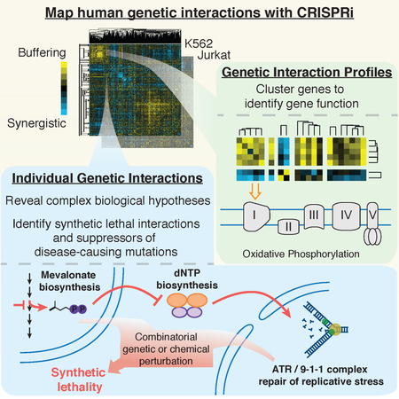
Seminal yeast studies established the value of comprehensively mapping genetic interactions (GIs) for inferring gene function. Efforts in human cells using focused gene sets underscore the utility of this approach, but the feasibility of generating large-scale, diverse human GI maps remains unresolved. We developed a CRISPR interference platform for large-scale quantitative mapping of human GIs. We systematically perturbed 222,784 gene pairs in two cancer cell lines. The resulting maps cluster functionally related genes, assigning function to poorly characterized genes, including TMEM261, a new electron transport chain component. Individual GIs pinpoint unexpected relationships between pathways, exemplified by a specific cholesterol biosynthesis intermediate whose accumulation induces deoxynucleotide depletion, causing replicative DNA damage and a synthetic-lethal interaction with the ATR/9-1-1 DNA repair pathway. Our map provides a broad resource, establishes GI maps as a high-resolution tool for dissecting gene function, and serves as a blueprint for mapping the genetic landscape of human cells.

Graphical Abstract

In brief

A large-scale genetic interaction map in human cells reveals unexpected interdependencies between core pathways and exposes potential combination therapies for cancer

INTRODUCTION

A powerful approach to objectively and systematically identify gene function is to map genetic interactions (GIs)—pair-wise measurements of how the activity of one gene modulates the phenotype of another gene. Applied broadly across many pairs of functionally diverse genes, GI maps provide a signature of interactions for each gene that act as a high-resolution, quantitative phenotype. This signature can be used to objectively identify genes with similar functions without any a priori assumptions. The pattern of GIs can also reveal the hierarchical organization of gene products into functional complexes and pathways (Collins et al., 2007).

By far the most mature efforts to exploit GI maps have been in the budding yeast S. cerevisiae. Pioneering work from Boone and colleagues enabled the first large-scale measurement of GIs (Tong et al., 2001,2004). Early GI maps demonstrated the broad utility of such efforts in enabling functional discoveries including the identification of uncharacterized protein complexes, cellular quality control and regulatory strategies, as well as unrecognized biosynthetic pathways (Collins et al., 2007; Jonikas et al., 2009; Pan et al., 2004, 2006; Schuldiner et al., 2005; Segrè et al., 2005). GI maps also revealed functional rewiring in yeast response to DNA damage or autophagy stress (Bandyopadhyay et al., 2010; Kramer et al., 2017). More recently, hallmark papers in S. cerevisiae revealed the first and only comprehensive functional genetic landscape of a cell (Costanzo et al., 2010, 2016). Additionally, GI mapping efforts in prokaryotes, as well recent work in S. pombe, fruit fly and human cells, demonstrate the general utility and enormous promise of GI maps across diverse organisms (Babu et al., 2014; Bassik et al., 2013; Boettcher et al., 2018; Du et al., 2017; Fischer et al., 2015; Frost et al., 2012; Han et al., 2017; Roguev et al., 2007, 2013; Rosenbluh et al., 2016; Shen et al., 2017; Wong et al., 2016).

Given the success of yeast studies, as well as focused efforts in mammalian cells, it is clear that large-scale GI maps of human cells could be transformative tools for facilitating the systematic elucidation of the function of protein coding and non-coding genes as well as revealing higher-level principles of cellular organization. Additionally, large-scale GI maps can aid the design of therapeutic efforts both by identifying synthetic-lethal combinations, which can enable rational design of combination therapies, as well by identifying buffering or suppressive interactions, which can provide molecular targets whose inhibition will ameliorate the consequences of genetic mutations. However, the broader goal of mapping diverse cellular processes in vertebrates comprehensively remains unmet.

Multiple challenges have limited large-scale GI mapping efforts in human cells. There are an enormous number of possible gene pair combinations to query (~200 million for a mammalian cell), and strong GIs are typically rare (Hartman et al., 2001). Thus, generating quantitative genetic interaction maps require a method for robustly perturbing a given gene’s functions while avoiding heterogeneity and off-target effects. Additionally, for large numbers of gene pairs, one must be able to precisely measure the effect of each genetic perturbation and quantitatively evaluate the observed defect for a gene pair relative to that expected from the phenotypes of the individual perturbations. These challenges have been mitigated by preselecting smaller subsets of functionally related genes (e.g., involved in chromatin-regulation, toxin resistance, regulators of β-catenin activity, or cancer biology) (Bassik et al., 2013; Du et al., 2017; Han et al., 2017; Roguev et al., 2013; Rosenbluh et al., 2016; Shen et al., 2017; Wong et al., 2016) (Table S1). However, it remains unresolved whether a GI map of diverse human genes can generate a GI signature enabling one to cluster genes by function and assign function to poorly characterized genes.

Here, we describe a mammalian GI mapping platform, based on CRISPR interference (CRISPRi), in which the expression of targeted genes is specifically repressed using a catalytically dead version of Cas9 (dCas9) fused to a KRAB transcriptional repression domain, allowing for precise and homogenous gene knockdowns (Gilbert et al., 2013, 2014; Horlbeck et al., 2016a). We present a combined experimental and analytic framework for high-precision, ultra-rich GI mapping and apply this platform to create a high-content, large-scale GI map of human genes that are diverse with respect to function and localization of the encoded proteins. Our GI map contains 1,044,484 sgRNA pairs targeting 222,784 gene pairs, which greatly increases the number of genetic interactions measured in human cells (Table S1). Our GI platform reveals high-content GI signatures that enable us to group related genes and assign function to even poorly characterized genes in an unbiased manner. Our CRISPRi GI map also delineates known and new GIs in pathways and protein complexes across diverse cellular processes, revealing unexpected biological principles and demonstrating that this method is well suited for systematic functional analysis of mammalian cells. We further show that GI maps can be used to identify robust genetic suppressors and synthetic sick/lethal (SSL) gene pairs, which point to therapeutic strategies for human diseases. Our maps are both a broad resource and a demonstration that large-scale CRISPRi GI maps can systematically elucidate how sets of genes encode the biology of protein complexes, pathways and organelles in human cells, providing both the motivation and an experimental and analytic framework for constructing a GI map of the entire human cell.

RESULTS

A CRISPRi Platform for Mapping GIs in Human Cells

We devised a strategy for creating loss-of-function GI maps in human cells using CRISPRi-expressing cells transduced with dual sgRNA lentiviral vectors to screen for pairwise sgRNA phenotypes (Figure 1A). CRISPRi has several unique properties that facilitate GI mapping efforts (Gilbert et al., 2014; Horlbeck et al., 2016a; Liu et al., 2017; Qi et al., 2013). Unlike nuclease-active CRISPR/Cas9, CRISPRi does not produce in-frame indels which can generate partially active proteins (Wong et al., 2016). In pooled functional genomic screens, in-frame indels have been shown to generate phenotype heterogeneity that will be compounded by simultaneously targeting more than one gene (Shalem et al., 2015). We have shown by population and single-cell RNA sequencing that CRISPRi can be used to effectively, specifically, and homogeneously silence the expression of up to 3 genes simultaneously (Adamson et al., 2016). Lastly, CRISPRi activity does not generate DNA double stranded breaks that activate a DNA damage response and can lead to non-specific toxicity phenotypes (Wang et al., 2015).

Figure 1. A large-scale quantitative GI mapping platform in human cells.

(A) Schematic of the overall GI mapping approach. (B) Histogram of gene growth phenotypes (γ) from a CRISPRi v1 growth screen (Gilbert et al., 2014). A subset of these genes were selected for inclusion in the GI map based on exhibiting a moderate growth phenotype and a high-confidence p-value. (C) Cellular processes represented in GI map, with number of genes in parentheses (see also Table S2). (E) Approach for quantifying epistasis between sgRNAs, based on the relationship between single sgRNA phenotypes and the corresponding pair phenotypes with a given “query” sgRNA. (F) Example of sgRNA epistasis with query sgRNA sgANAPC13-1. Negative control sgRNAs are circled in red, and red line corresponds to quadratic fit of all sgRNA single and pair phenotypes (see also Figure S3A).

To construct GI maps, we developed a barcoded, dual-sgRNA lentiviral vector that enabled us to robustly silence pairs of genes and then track each perturbation in a pooled CRISPR screen (Figure S1A). Recombination has been shown to confound quantitative genetic analysis by scrambling nucleic acid information (Du et al., 2017; Han et al., 2017). To avoid this issue, we developed a new sequencing strategy and analysis pipeline we named “triple sequencing” that sequences both the barcodes and the sgRNAs encoded by each DNA molecule, allowing us to identify and discard in silico all recombination events (Figure S1A and see Methods).

A GI Map of Diverse Cellular Processes

We constructed a large loss-of-function GI map primarily by selecting sgRNAs targeting genes that we previously identified in a CRISPRi screen as essential for robust cell proliferation or viability (see Methods, Figure 1B, and Table S2) (Gilbert et al., 2014). As demonstrated in yeast, partial loss-of-function genetic methods, such as CRISPRi, are particularly well suited for the study of essential genes (Costanzo et al., 2016; Schuldiner et al., 2005). The genes in our map represent diverse cellular processes localized to all major intracellular compartments (Figure 1C and Table S2). We used a custom cloning strategy to construct a dual sgRNA library of 1,044,484 pairwise CRISPRi genetic perturbations targeting 222,784 gene pairs (472 genes × 472 genes) representing 111,628 unique combinations (Figure 1A and S1A-C).

We transduced K562 cells stably expressing dCas9-KRAB with our GI library in replicate and conducted two independent cell growth screens to measure how each sgRNA pair perturbs cell proliferation (Figure S1B-D). Using triple sequencing, we measured the growth phenotype (γ) of sgRNA pairs based on their relative abundances at the start (day 5 post-infection, referred to here as T0) and end of the screen, normalized to the number of cell doublings (Figure S2A). Our triple sequencing analysis clearly revealed recombination between the A and B sgRNA positions in our vector, with ~5% of sgRNA A and the corresponding barcode mismatched and ~16% of sgRNA B and barcode mismatched, proportional to the distance between those elements in the lentiviral vector. We used this strategy to remove recombination products, thus correcting this artifact that limited the dynamic range of our screen phenotypes (Figure S2B-D and Table S3).

We also performed the GI screen in Jurkat cells using the same library and approach (Figure S2E-F). The triple sequencing correction had minimal impact prior to phenotypic selection (i.e., T0) but had a substantial effect at the screen endpoint (Figure S2G-H). We filtered from further analysis a subset of sgRNAs that produced growth phenotypes in K562 but not in Jurkat cells (Figure S2I and Table S4).

We then calculated sgRNA- and gene-level interactions from the sgRNA pair phenotypes based on a GI paradigm previously established for yeast and shRNA GI screens (Bassik et al., 2013; Collins et al., 2007; Jonikas et al., 2009; Kampmann et al., 2013; Schuldiner et al., 2005) (Figure S1D). For a given “query” sgRNA, buffering or synergistic (i.e. SSL) interactions were calculated based on the deviation of the observed double-sgRNA phenotype from the expected phenotype (Figure 1D-E). In our dataset, we found that a quadratic fit of single vs. pair sgRNA phenotypes best modeled the expected phenotype (Figure S3A-B).

Five observations argue for the validity and reproducibility of the measured sgRNA GIs in K562 and Jurkat cells. First, GIs for each replicate screen are well correlated especially when GIs distributed near zero, which represent gene pairs that do not interact, are masked (Figure 2A and Table S5). Second, sgRNA GI profiles show substantial correlation across independent replicate screens (R=0.75 and 0.44 for K562 and Jurkat respectively; Figure 2B, S3C). Third, sgRNAs targeting the same gene correlated well (the median same-gene sgRNA correlation was 8-fold stronger than background in K562, Figure 2C). Fourth, sgRNAs targeting genes in the same biological complex are similarly well correlated, with the caveat that for extremely sick sgRNA pairs, it is difficult to accurately measure a GI signature (Figure 2B-C, S3C, and interactive sgRNA-level GI map files). Finally, we experimentally validated a number of buffering and SSL GIs in K562 and Jurkat (Figure S4A-F, and Table S6).

Figure 2. A large-scale CRISPRi-based GI map.

(A-B) sgRNA GI scores (A) and GI correlations (B) from two independent replicates performed in K562. Contours correspond to 99th, 95th, 90th, 75th, 50th, and 25th percentiles of data density. Pearson correlation (R) is of all sgRNA pair correlations. Due to the size of the dataset, Pearson P-values here and throughout the manuscript are < 10⁻³⁰⁰ unless otherwise stated. (C) Histogram of sgRNA GI correlations calculated from replicate-averaged sgRNA pair phenotypes. Smoothed histograms of all pairs of sgRNAs or only sgRNA pairs targeting the same gene or complex were generated with Gaussian kernel density estimation. (D-E) Gene-level GI scores (D) and GI correlations (E), displayed as in A-B. (F) Histogram of gene GI correlations from replicate-averaged screens, displayed as in C. (G) Full gene-level GI map in K562. Dendrogram indicates average linkage hierarchical clustering based on uncentered Pearson correlations between genes. Clusters were annotated by assigning GO annotations if the GO term was significantly enriched in that cluster (hypergeometric P ≤ 10⁻⁹) and not more enriched in another cluster.

To construct gene-level GI maps, we first averaged interactions for all sgRNA pairs targeting a given gene pair. Gene-level GI scores and GI correlations correlated well, and as with sgRNA-level interactions, intra-complex gene pairs were much more highly correlated than background (Figure 2D-F, S3D, and Table S5). The magnitude of intra-complex correlations varies by complex, which may be due to the challenge of GI mapping for highly essential gene pairs or may point to functionally distinct complex subunits or sub-complexes (Bassik et al., 2013; Collins et al., 2007). Our analysis also shows that GI maps containing more than 1 sgRNA per gene will boost signal-to-noise at the cost of larger double-sgRNA libraries (see Mendeley extended data [doi:10.17632/rdzk59n6j4.1]).

GI Maps Cluster Genes by Function

GI maps give two distinct types of information: clustering of genes by similarities of their profile of GIs informs assignment of genes to complexes, pathways, or processes; specific GIs reveal functional connections between gene pairs (Figure 1A). Here, we first describe the structure and insights gained from gene clustering and then discuss the analysis and hypotheses generated by GIs below.

Hierarchical clustering of our K562 and Jurkat GI maps demonstrates the power of GI mapping for the functional characterization of human genes of diverse or unknown functions (Figure 2G and see Mendeley[doi:10.17632/rdzk59n6j4.1] for annotated Jurkat map and interactive GI heatmaps and network diagrams). We used a systematic approach to annotate the clusters enriched for genes known to act in a given complex, process, or cellular compartment, assigning Gene Ontology (GO) annotations for clusters at any level of the hierarchy if a given GO term was enriched relative to the full GI map at P≤10⁻⁹, and if it was more enriched than at any other cluster. This identified 33 functionally coherent clusters in K562 at the highest resolution, each containing between 2 and 19 genes (Figure 2G). The same approach in the smaller Jurkat map found 22 clusters and recapitulated many of the same GO-annotated clusters found in K562, highlighting the consistency of these findings. Prominent highlights include a mitochondrial supercluster with clear sub-clusters functionally defining mitochondrial metabolism genes, mitochondrial protein translation, and Complex I of the Electron Transport Chain (ETC), indicating that our GI mapping platform can reveal interconnected functional processes within an organelle (see Mendeley[doi:10.17632/rdzk59n6j4.1] for GI map excerpts). We also observe two large clusters of genes involved in the secretory pathway and in mitosis. We note that repression of several of the ER Membrane Complex (EMC) genes does not confer a primary growth phenotype; however, all EMC genes cluster well together (see Mendeley[doi:10.17632/rdzk59n6j4.1] and see Methods). Future maps targeting genes without primary phenotypes will require robust sgRNA activity predictions. We find that even with genes previously found to be difficult to target (Du et al., 2017), 2 of every 3 sgRNAs predicted to be highly active by our current algorithm gave greater than 90% repression of the target gene, and all gave greater than 75% repression (Figure S4G) (Horlbeck et al., 2016a). Finally, we reanalyzed both our sgRNA-level and gene-level maps while systematically excluding large clusters of genes, limiting GIs to only buffering or SSL, or greatly reducing the dynamic range of the GI scores, and found that clustering of the map was robust to each of these perturbations suggesting that GI correlations are driven by broad trends in the GI map rather than specific interactions (Figure S5A-E).

GI Maps Reveal a High Degree of Unannotated Gene Function in Human Cells

To explore the ability of correlations to uncover new functional relationships more systematically, we next analyzed the distribution of GI profile correlations (Figure 3A). The large majority of gene pairs showed poor correlation, as expected; however, many gene-gene correlations were stronger than any gene-negative control correlation (20,464 correlations > 0.178, 20.4% of all interactions), suggesting enrichment for functional relationships. Gene correlations within a given cellular compartment were enriched for strong correlations compared to the total distribution or to cross-compartment relationships (Figure 3B), and highly correlated gene pairs were enriched for known physical interactions annotated by the STRING physical interaction database (Figure 3C and S5F). Notably, many of the most highly correlated gene pairs were not captured by STRING annotation (315 unannotated pairs of 390 at GI correlation > 0.6), suggesting both unidentified physical interactions and functionally related genes that do not physically interact (Figure 3C). Conversely, GI correlations captured the majority of STRING-annotated interactions (79.3% of highest confidence interactions at GI correlation > 0.1; Figure S5F) and also could predict gene pairs that frequently co-occurred in GO terms (Figure S5G). Between K562 and Jurkat, we found that both the GI profiles for each gene and the gene-gene GI correlations within each cell line were well correlated (Figure 3D-E).

Figure 3. GI correlations identify members of protein complexes and functionally related pathways.

(A) Histogram of all correlations between K562 gene GI profiles (green) or between non-targeting (NT) control and gene GI profiles (black). (B) Cumulative distribution of GI correlations for all genes (as in A), for gene pairs within mitochondria or early trafficking, or for pairs with one gene in each compartment. (C) Fraction of gene pairs with a given GI correlation annotated by the STRING experimentally validated interaction set. GI correlations were binned to the next-lowest tenth. (D) Histogram of the correlations between GI score profiles in K562 and Jurkat maps. Only genes present in both K562 and Jurkat are included. (E) Comparison of GI correlations within each GI map. (F) Gene networks of the most highly correlated genes in K562. Edges represent correlations greater than 0.6. GI correlations that correspond both to STRING-annotated interactions and to MitoCarta gene pairs were labeled according to their STRING interaction confidence. Edge lengths were determined by force-directed layout. Asterisks indicate gene pairs that have closely neighboring TSSs.

To explore the ability our GI map to identify known and previously unannotated functional relationships further, we examined all 390 gene pairs with a correlation above 0.6 in the K562 GI map. Within this set of highly correlated genes, we found strong enrichment for genes that encode physical protein complexes annotated by STRING (grey lines, Figure 3F). We also observed highly correlated gene pairs (166 of all 390 top correlated gene pairs) that were not annotated to interact but were both annotated as important for mitochondrial function in MitoCarta (purple lines, Figure 3F). We also noted that two gene pairs with unannotated associations have closely neighboring gene transcription start sites (TSS). We and others have shown CRISPRi can repress expression of TSSs within ~1kb of the target site, so in these cases orthogonal methods are required to separate the contribution of each gene perturbation to the GI profile (Figure 3F starred pairs, S5H-I). We have annotated all gene pairs within the map that could have a neighbor effect that convolutes analysis (Table S2). Even after considering STRING, MitoCarta, and neighboring genes, we identified 35 unannotated functional associations at this high threshold of GI correlation (red lines, Figure 3F).

Further inspection of these 35 unannotated functional correlations reveals novel predictions for ER protein trafficking, DNA synthesis, and the ETC. For example, we identify a strong correlation between the genes ASNA1 and CAMLG. ASNA1/CAMLG are homologous to the yeast genes GET3/2; we provide unbiased in vivo support that these genes coordinate protein import to the ER (see Mendeley[doi:10.17632/rdzk59n6j4.1] GI map excerpts). We also identify strong GI correlations associated with canonical DNA replication genes such as between POLE2 and PRIM2 as well as POLD1, POLD3 and CACTIN (Figure 3F). We were intrigued by the strong correlation of CACTIN within a DNA replication gene cluster that includes canonical DNA replication genes such as POLD1, POLD3, POLE, MCM3, MCM4, RFC4 and RFC5 (Figure 2G). While the biology of CACTIN is poorly characterized, it is evolutionarily conserved and physically associated with the spliceosome (Baldwin et al., 2013). In our GI map, the CACTIN GI profile is more strongly correlated (R > 0.6) with DNA replication genes than with core splicing factors (R = 0.16–0.32), although a number of genes considered to be splicing cofactors correlate well with CACTIN (see Mendeley[doi:10.17632/rdzk59n6j4.1] extended data for CACTIN analysis and validation). We provide support for similarities between loss of CACTIN and core components of DNA polymerase ∂ Repression of CACTIN more closely phenocopies repression of polymerase ∂ subunits than several tested splicing factors. Specifically, repression of CACTIN and POLD1/3 results in S phase arrest, decreased DNA replication, and activation of CHEK1 S345 phosphorylation (p-Ser345 CHEK1), a hallmark of DNA damage signaling activated by defects in DNA replication (Harper and Elledge, 2007).

We were also intrigued by the observation that the poorly characterized gene TMEM261 is most strongly correlated with four ETC Complex I genes present in the K562 GI map and also exhibits buffering genetic interactions with these and other genes functioning in the TCA cycle and ETC in K562 and Jurkat (Figure 2G, 3F, 4A and see Mendeley[doi:10.17632/rdzk59n6j4.1]).Validation studies revealed that repression of TMEM261 decreased ATP levels in respiratory but not glycolytic conditions in a manner quantitatively indistinguishable from repression of core Complex I genes (Figure 4B). Together with recent physical evidence showing that TMEM261 is associated with Complex I components (Stroud et al., 2016), our data suggest TMEM261 is indeed a functionally critical component of Complex I.

Figure 4. Oxidative metabolism is highly correlated with poorly characterized gene TMEM261 and anti-correlated with glycolytic metabolism.

(A) Selected GIs with mitochondrial complex I and glycolytic genes from the K562 GI map. (B) ATP levels relative to baseline ATP following one-hour incubation in either respiratory or glycolytic conditions. Data show mean ± SEM, and N=16 experimental replicates per group from two independent experiments. *** indicates P<0.001 versus NT sgRNA in each condition by one-way ANOVA with Dunnett’s multiple comparisons test. (C) GI scores for genes paired with ATP5A1 and PGK1. (D) GI correlation with ATP5A1 for genes involved in carbon metabolism.

We also observed that the GI pattern for glycolytic genes, such as PGD and PGK1, was anti-correlated with TMEM261 as well as with other genes required for oxidative phosphorylation (OX-PHOS). In one highlighted example, we found that PGK1 was strongly anti-correlated with ATP5A1 (R = −0.53), a core component of ATP synthase. Repression of ATP5A1 is buffering with repression of genes required for mitochondrial processes such as OX-PHOS, while repression of PGK1 results in a synergistic phenotype with the same genes (Figure 4C). Broadly, genes upstream of the TCA cycle were anti-correlated with ATP5A1, while genes downstream of the TCA cycle were correlated with ATP5A1 (Figure 4C-D). We measured ATP produced by respiration or by glycolysis upon knockdown of PGK1. Surprisingly, repression of PGK1 reproducibly increased the amount of ATP produced by respiration, while ATP associated with glycolysis was unchanged (Figure 4B). Although additional experiments will be required to elucidate the underlying biology, we believe these experiments support the anti-correlated phenotype in the GI map and we hypothesize that the anti-correlated gene sets reveal unanticipated bioenergetic regulation.

The Structure of GIs in Human Cells

Finally, we investigated the overall structure of GIs. We first analyzed the distribution of gene-negative control interactions in our K562 dataset and used this to both define a 5% FDR threshold for GIs as well as a “strong” GI cut-off of +/− 3, essentially beyond the distribution of all negative controls (Figure S6A). By this definition, strong GIs are rare, representing just 2.2% of total gene-gene interactions measured (Figure 5A). The frequency of strong GIs in human cells is similar to the frequency observed in yeast (Costanzo et al., 2010; Schuldiner et al., 2005), although we note that our gene set is enriched for genes required for cell growth and therefore may not reflect an average frequency of GIs across all genes. We observed that strong buffering interactions are most frequent between genes with highly correlated GI profiles, while synergistic interactions were found across all levels of GI correlation (Figure 5B). These GI observations are recapitulated in our Jurkat GI map (Figure S6C-E).

Figure 5. Structure of genetic interactions in the GI map.

(A) Histogram of all GI scores between unique gene pairs in K562. Same-gene pairs were not included. (B) Relationship between GI correlation and GI score. GI correlations were binned to the next-lowest tenth. (Left) Boxplot of scores within each bin. (Middle) Percent strong buffering interactions within each bin. (Right) Percent strong synergistic interactions within each bin. (C) Enrichment of correlations and strong interactions for gene pairs between the indicated cellular compartments. Values indicate the percent of all gene pairs between the compartments that are correlated or have a GI score above the stated thresholds. (D) Average GI score between GO-annotated clusters in the K562 GI map. Clusters correspond to those displayed in Figure 2G. Numbers in parentheses indicate number of member genes.

GI correlations between gene pairs are most enriched within genes encoding proteins localized to specific cellular compartments (Figure 5C). Strong buffering interactions mirror this distribution and are enriched within certain cell compartments, while for SSL interactions there is less enrichment for interactions within subcellular compartments. Instead, we see the majority of SSL interactions occur across subcellular compartments (Figure 5C). Gene pairs that co-occurred in GO annotations were also enriched among the strongest buffering and SSL interactions (Figure S6B), but to a lesser extent than among gene pairs with the highest GI correlations (Figure S5G).

While the above analysis reflects the trend of strong interactions across the full dataset, we asked whether this observed structure holds true at the level of functional clusters. Using the GO-annotated clusters presented in Figure 2G, we calculated average GIs within clusters and between clusters across all levels of the cluster hierarchy. Within clusters, average GIs were broadly distributed but most were SSL rather than neutral or buffering, consistent with findings in yeast for essential gene clusters (Figure S6F) (Costanzo et al., 2016). The nature of genes present in the map dictates these observed GI relationships and will need to be evaluated in a genome-scale human GI map. This analysis also revealed strong and coherent GIs between both closely related gene sets and across disparate processes (Figure 5D and S6F). Comparative analysis of cluster-cluster interactions in K562 and Jurkat cells found that average GIs were highly correlated (R=0.62), but also highlighted instances of possible functional rewiring (Figure S6G). In one intriguing example, we observed a strong buffering interaction between the MICOS complex and ATP synthase in Jurkat but not K562 despite conservation of a strong TIMM9/22 buffering interaction with MICOS in both lines. This may represent a differential requirement for maintenance of the oxidation of the intermembrane space or for the assembly of ATP synthase. Our cluster-level analysis also highlighted numerous interactions mediated by components of the PAF1 transcription control complex, which represent a substantial fraction of the both the top buffering and synergistic cluster pairs (Figure S6F).These include suppressor interactions between repression of LEO1, a component of the PAF1, and mitochondrial dysfunction induced by repression of essential mitochondrial genes (Figure S6H-I). We experimentally validated strong buffering interactions between LEO1 and several mitochondrial genes (Figure S6J-K). Broadly, these findings emphasize that GI maps can reveal unexpected genetic perturbations that suppress the phenotype of a loss-of-function mutation.

Accumulation of a Specific Metabolite in Cholesterol Biosynthesis Causes Replicative DNA Damage

A major goal of GI maps is to uncover unexpected synergistic and buffering interactions that can drive new discoveries in cell biology and inform the design of therapies (Hartman et al., 2001). With that in mind, we were intrigued by an unexpected SSL interaction between HUS1, a gene encoding a component of the 9-1-1 cell-cycle checkpoint response complex that plays a major role in DNA repair, and FDPS, an enzyme in the mevalonate pathway that catalyzes production of farnesyl pyrophosphate, an intermediate product in sterol biosynthesis (Figure 6A) (Cerqueira et al., 2016; Harper and Elledge, 2007). Also evident in our GI map were SSL interactions between HUS1 and other DNA repair genes, between FDPS and the EMC complex, and between both FDPS and HUS1 and RRM1, the catalytic subunit of the ribonucleotide reductase complex (RNR), required for deoxynucleotide production (Figure 6A) (Arnaoutov and Dasso, 2014). We validated the SSL between FDPS and HUS1 (Figure 6B). Intriguingly, HUS1 is not SSL with repression of PMVK, an enzyme upstream of FDPS in the canonically linear mevalonate biosynthetic pathway (Figure 6A,C). As PMVK and FDPS are the only genes annotated to be in the mevalonate pathway in our GI map, this either represents an artifact in the GI map or points to a specific interaction between HUS1 and FDPS rather than HUS1 and the mevalonate biosynthesis pathway.

Figure 6. Repression of FDPS is synthetic lethal with HUS1 and results in accumulation of the cholesterol intermediate IPP.

(A) Selected interactions with HUS1 and with FDPS in the K562 GI map. (B) Individual validation experiments sgRNAs targeting HUS1 and FDPS, performed as in Figure S4A. Lines represent mean of two experimental replicates (open circles). (C) Schematic of the cholesterol biosynthesis pathway. Gene names are colored by mean validation GI (see also Figure 6D) of all sgRNA pairs targeting HUS1 and the indicated gene. (D) sgRNA pair epistasis for sgRNAs targeting HUS1 and cholesterol biosynthesis genes. Epistasis was calculated as the measured double-sgRNA phenotype subtracted by the sum of the individual phenotypes and by epistasis with non-targeting (NT) sgRNA. Bars represent mean of duplicate experiments and error bars represent the maximum and minimum data points. (E) Epistasis between sgRNAs targeting HUS1 and FDPS in the presence of DMSO control or 4 μM lovastatin. (F) IPP concentration in cells containing NT or FDPS-targeting sgRNAs grown in the presence or absence of 4 μM lovastatin for 48 hours. N=6 replicates each (4 for lovastatin-treated samples).

To elucidate this discrepancy, we systematically repressed each gene in mevalonate biosynthesis and the pathway leading to cholesterol and other biosynthetic products. Repression of only FPDS and IDI1 was SSL with HUS1 knockdown, validating our GI map results and suggesting that repression of the mevalonate pathway per se is not SSL with HUS1 (Figure 6C-D, S7A-C). Rather, because FDPS and IDI1 both utilize the metabolite isopentenyl pyrophosphate (IPP), our results suggest that accumulation of IPP resulting from repression of FDPS or IDI1 leads to DNA damage. To further support this conclusion, we used lovastatin, a chemical inhibitor of HMGCR, an enzyme upstream of PMVK, FDPS and IDI1 in the mevalonate biosynthesis pathway, or alendronate, a chemical inhibitor of FDPS, to recapitulate this genetic phenotype (Bergstrom et al., 2000). We found that chemical inhibition of HMGCR by lovastatin does not interact with repression of HUS1, consistent with the genetic data. By contrast, lovastatin strongly buffers growth defects induced by genetic or chemical repression of FDPS activity (Figure S7D-E). This implied that lovastatin was likely preventing accumulation of IPP, a potentially toxic metabolite, and that the observed phenotypes do not relate to sterol biosynthesis or protein prenylation, a proposed mechanism for alendronate cytotoxicity (Bergstrom et al., 2000)

If IPP is indeed responsible for the SSL interaction between HUS1 and FDPS/IDI1, then inhibition upstream of FDPS should also rescue the genetic interaction between HUS1 and FDPS. We knocked down both HUS1 and FDPS in the presence or absence of lovastatin and observed that, as predicted, inhibition of HMGCR rescues the SSL phenotype between HUS1 and FDPS, providing strong support for the hypothesis that IPP drives this SSL phenotype with HUS1 (Figure 6E). In further support of this hypothesis, we observed that IPP levels are strongly induced upon knockdown of FDPS and this accumulation of IPP is blocked by inhibition of HMGCR with lovastatin (Figure 6F).

To explore the mechanism by which accumulation of IPP leads to DNA damage, we genetically or chemically repressed FDPS activity in disparate cell lines (K562, HEK293 and iPSC) and then measured p-Ser345 CHEK1, a canonical molecular marker of DNA damage signaling induced by DNA replication stress and DNA damage (Harper and Elledge, 2007). We observed that repression of FDPS induced an increase in p-Ser345 CHEK1, suggesting decreased FDPS activity is associated with activation of DNA damage signaling (Figure 7A-B). Importantly, repression of HUS1 does not induce p-Ser345 CHEK1. To further demonstrate that a specific metabolite in the mevalonate biosynthetic pathway drives activation of DNA damage signaling, we chemically inhibited both FDPS and HMGCR and observed that lovastatin rescues induction of p-Ser345 CHEK1 by alendronate (Figure 7C).

Figure 7. Chemical and genetic perturbation of FDPS causes replicative DNA damage via deoxynucleotide depletion.

(A) Western blot measuring CHEK1 and CHEK1 p-S345 abundance in K562 cells expressing sgRNAs targeting HUS1 or FPDS. (B) Western blots measuring CHEK1 and CHEK1 p-S345 abundance in K562, HEK293T, and iPSC cells treated with the indicated concentrations of alendronate. (C) Western blots measuring CHEK1 and CHEK1 p-S345 abundance in K562 treated with 4 μM lovastatin, 200 μM alendronate, or both drugs. (D) Sensitivity or resistance to alendronate induced by CRISPRi repression of genes involved major DNA repair pathways, excerpted from an unbiased alendronate screen in K562 cells (see methods and Table S7). (E) Cell cycle analysis of K562 cells before and after treatment with 250 μM alendronate. Cells undergoing DNA synthesis incorporate EdU and propidium iodide labels overall DNA content. (F) Sensitivity or resistance to alendronate induced by CRISPRi repression of genes that modify RNR activity, as in Figure 7D. P-values were calculated by Mann-Whitney test of all 10 sgRNAs targeting a given gene compared to negative controls; * indicates P<0.05, *** indicates P<0.001. (G) dATP and ATP concentration in K562 cells expressing NT or FDPS-targeting sgRNAs grown in the presence or absence of 4 μM lovastatin, measured by LC-MS/MS as in Figure 6F. N=6 replicates each (4 for lovastatin-treated samples). *** indicates P<0.001. (H) Schematic of proposed mechanism of FDPS/RRM1/HUS1 synthetic interactions. Red lines indicate the observed consequences of chemical and/or genetic perturbations.

To better understand the nature of the DNA damage induced by accumulation of IPP, we surveyed the sensitivity of cells to alendronate following knockdown of key components of each major DNA repair pathway. We observed that repression of the ATR signaling or 9-1-1 DNA repair, but not other DNA damage signaling or repair pathways, strongly sensitizes cells to chemical inhibition of FDPS activity (Figure 7D). ATR and the 9-1-1 complex are hallmark proteins required for repair of replicative DNA damage (Harper and Elledge, 2007). In support of this, we found that chemical inhibition of FDPS by alendronate induces S-phase arrest and decreases DNA synthesis, which, together with our genetic and signaling data, is consistent with the hypothesis that accumulation of IPP induces replicative DNA damage (Figure 7E).

Our GI map revealed that repression of RRM1 is synthetic lethal with repression of both FDPS and HUS1 (Figure 6A). We also observed repression of RRM1 and to a lesser extent RRM2 but not its p53-inducible homolog RRM2B sensitizes cells to alendronate while repression of AHCYL1, a negative regulator of RNR (Arnaoutov and Dasso, 2014), promotes resistance to alendronate (Figure 7F). Together, these genetic data suggest that the accumulation of IPP resulting from repression of FDPS directly or indirectly inhibits RNR, leading to decreased dNTP levels and replicative DNA damage. To test this hypothesis, we repressed FDPS and measured cellular nucleotide and deoxynucleotide levels. Knockdown of FDPS causes decreased levels of dATP and dCTP but not NTPs (Figure 7G and Figure S7F). Consistent with the idea that IPP accumulation leads to decreased dNTP levels, addition of lovastatin reversed the depletion of dATP and dCTP induced by FDPS knockdown (Figure 7G and Figure S7F).

These data support the detailed hypothesis suggested by the GI map data, in which increased IPP decreases the cellular pool of the dNTPs, leading to replicative DNA damage that must be sensed and repaired for viability (Figure 7H). Decreased dNTP levels must result from either a decrease in dNTP production by RNR or an increase in dATP degradation or consumption. Allosteric regulation of RNR is complex and it is tempting to speculate that IPP, a pyrophosphate, is an allosteric modulator of RNR activity.

These experiments illustrate the potential of GI maps to reveal unexpected druggable SSL GIs between genes that do not have a known physical association or correlated GI phenotype. Our work demonstrates we can use GI maps as a high-precision tool to decipher the cellular consequences of re-wired or dysregulated metabolic processes with clinical implications, since bisphosphonates, such as alendronate, are widely used to treat osteoporosis as well as bone metastatic prostate cancer and breast cancer.

Discussion

Here we present a combined experimental and analytic framework for high-precision ultra-rich GI mapping. We apply this platform to create two high-content large-scale GI maps of functionally and spatially diverse human genes each targeting 222,784 gene pairs. Our maps serve as a broad resource, and our experimental and analytic platform will enable future GI mapping efforts. Analysis of these GI maps supports three main conclusions.

First, we establish mammalian GI maps as a powerful tool for the unbiased functional characterization of highly diverse genes. The GI signature of a gene yields a high-resolution phenotype enabling one to robustly cluster genes of known biological function and assign function to poorly characterized genes. Specifically, principled annotation of our GI map revealed 33 high-resolution distinct functional gene clusters spanning diverse biological processes such as mitochondrial protein translation, electron transport, ER/Golgi protein trafficking, kinetochore and centromere biology and DNA replication. We highlight several novel functional inferences from GI signatures in our map, establishing the ability of this approach to reveal new biology not anticipated by other methods. Within a cluster, buffering GIs can be used to identify highly related genes as exemplified here by TMEM261 and Complex 1 of the ETC. We also show that most, but not all, gene pair GI correlations are conserved between two related hematopoietic cancer cell types.

Second, we establish the ability to identify unexpected SSL and buffering gene pairs to link diverse processes and dissect complex pathways. A striking example of an unexpected SSL link between disparate processes was the ability of systematic epistasis analysis to identify an endogenous chemical metabolite whose accumulation strongly enhances the cells dependence on an intact DNA damage response pathway. Further analysis of this SSL in our GI map revealed a complex hypothesis in which accumulation of a specific intermediate in cholesterol biosynthesis (IPP) causes deoxynucleotide depletion, which in turn leads to replicative DNA damage, S phase arrest, and thus exquisite dependence on an intact DNA damage response. Indeed, the specific pattern of GIs observed in the map supports each step of this hypothesis, which we have now verified with genetic, metabolomic and biochemical experiments. Identifying the mechanism of action of a metabolite in normal physiology or disease can be a daunting challenge. Building on the ability of genetic screens to pinpoint drug targets (Jost and Weissman, 2018), GI maps provide a strategy for linking a specific metabolite to its physiologic target by enabling one knock down to promote accumulation of a metabolite and the second to probe its physiological impact. Additionally, SSL and buffering interactions have important implications for the design of therapeutic strategies. For example, genetic suppressors of loss-of-function perturbations can guide development of therapeutic strategies for recessive loss-of-function diseases, and identification of SSL pairs can inform the design of combination therapies.

Third, at a broader level our data begins to shed light on the nature and frequency of GIs in human cells. Strong buffering and SSL interactions are rare and this scarcity illustrates the need for large-scale, systematic and robust methods such as GI mapping capable of identifying and characterizing interacting gene pairs. Expanding the analysis of GI frequency to more genes and cell types will provide insight into polygenic diseases as well as the role of GIs in contributing to missing inheritance seen in association studies (Manolio et al., 2009).

Our work provides a robust platform for future GI mapping efforts that will complement the rich insights obtained from recent large-scale efforts that use comparative genome-scale CRISPR or RNAi screens in the context of naturally occurring cancer-associated genome variations across cancer cell lines to define gene function (Hart et al., 2015; Tsherniak et al., 2017; Wang et al., 2017). Beyond the cancer genome, we envision applying CRISPR-based methods to model disease-associated cellular states (genomic variants, transcriptional profiling, epigenetic profiling) and then using GI maps to dissect specific disease states with high resolution. While we focus here on cell growth, we anticipate that these approaches can be applied to any quantifiable measure of cellular phenotype (e.g. expression of fluorescent reporters) (Adamson et al., 2016; Jonikas et al., 2009). Given the rich information from the present map and the precedent set by yeast, such efforts will be transformative for the study of normal biology and pathological states.

STAR METHODS

CONTACT FOR REAGENT AND RESOURCE SHARING

Further information and requests for resources and reagents should be directed to and will be fulfilled by the Lead Contact, Jonathan Weissman (Jonathan.Weissman@ucsf.edu).

EXPERIMENTAL MODELS: CELL LINES and LENTIVIRUS

All cell lines were cultured at 37°C 5% CO2 in standard tissue culture incubators. HEK293T (female) cells used for packaging lentivirus or for experiments were maintained in Dulbecco’s modified eagle medium (DMEM) in 10 % FBS, 100 units/mL streptomycin and 100 μg/mL penicillin with 2mM glutamine. K562 (female) and Jurkat (male) cells were grown in RPMI-1640 with 25mM HEPES and 2.0 g/L NaHCo3 in 10 % FBS, 2 mM glutamine, 100 units/mL streptomycin and 100 μg/mL penicillin (Gibco). WTC Gen1c iPSCs (male) were maintained under feeder-free conditions on growth factor-reduced Matrigel (BD Biosciences) and fed daily with mTeSR medium (STEMCELL Technologies) (Liu et al., 2017). Accutase (STEMCELL Technologies) was used to enzymatically dissociate iPSCs into single cells. To promote cell survival during enzymatic passaging, cells were passaged with the p160-Rho-associated coiled-coil kinase (ROCK) inhibitor Y-27632 (10 μM; Selleckchem). iPSCs were frozen in 90% fetal bovine serum (HyClone) and 10% DMSO (Sigma). Lentivirus was produced by transfecting HEK293T with standard packaging vectors using TransIT®-LTI Transfection Reagent (Mirus, MIR 2306). Viral supernatant was harvested 72 hours following transfection and filtered through a 0.45 μm PVDF syringe filter. To construct the CRISPRi K562 cell line, we lentivirally transduced K562 cells, originally obtained from ATCC, to stably express dCas9-BFP-KRAB (Gilbert et al., 2014). We then sorted the CRISPRi K562 cells by flow cytometry using a BD FACS Aria2 for stable BFP signal which marks dCas9-BFP-KRAB expression to create a pure polyclonal CRISPRi K562 line. CRISPRi Jurkat cells (Clone NH7) were obtained from the Berkeley Cell Culture Facility. WTC Gen1c iPSCs cells are a gift from Bruce Conklin. All cell lines were routinely tested for mycoplasma (MycoAlert, Lonza).

METHOD DETAILS

Plasmid design and construction

The GI sgRNA library vector is a modified version of a published sgRNA lentiviral plasmid (Figure S1A) (Horlbeck et al., 2016a). In the final GI library sgRNA vector, the 5’ sgRNA is expressed from a modified mouse U6 promoter while the 3’ sgRNA is expressed from a modified human U6 promoter (Figure S1A). Both sgRNAs expressed from this vector employ the same optimized S. pyogenes sgRNA constant region. The GI library sgRNA vector also encodes 4 randomized 16 base pair DNA barcodes allowing us to measure vector recombination by Illumina sequencing (Figure S1A). The GI lentiviral sgRNA construct co-expresses BFP and a puromycin resistance cassette separated by a T2A sequence from a Ef1Alpha promoter. The lentiviral sgRNA vectors for the dual color competition assay to confirm GI phenotypes are previously described but briefly each vector encodes a modified mouse U6 promoter that drives expression of the sgRNA described above as well as either GFP or BFP and a puromycin resistance cassette separated by a T2A sequence from an Ef1Alpha promoter.

We used previously described lentiviral vectors to express the CRISPRi dCas9-KRAB protein (Gilbert et al., 2013). The CRISPRi fusion encodes mammalian codon optimized S. pyogenes dCas9 (DNA 2.0) fused at the C-terminus with two SV40 nuclear localization sequences (NLS), BFP and the Kox1 KRAB domain expressed from either the SFFV or Ef1Alpha promoter.

GI library design

The gene set was obtained from all genes that had a growth phenotype (γ) less than −0.1 and greater than −0.3 in a CRISPRi v1 growth screen (Gilbert et al., 2014). Genes were further filtered to require that all genes had a “discriminant score” based on both effect size and P-value greater than 30 in our sgRNA activity dataset (Horlbeck et al., 2016b), to ensure that multiple sgRNAs targeting each gene were active. To evaluate whether these genes were also deleterious for growth when disrupted by CRISPR nuclease, genes in the GI map were checked against genes scoring above the cell line-specific Bayes Factor threshold from (Hart et al., 2015) and below adjusted P-value of 0.05 from (Wang et al., 2015). 90.6% of the CRISPRi v1 genes with negative growth phenotypes incorporated into the map were deleterious to growth in at least two of ten CRISPR nuclease screens, suggesting many of the genes in this gene set can be considered essential to cell viability in a range of contexts. Two sgRNAs targeting each gene were selected using the top two sgRNAs by activity score; in arbitrary cases, the third sgRNA was also included to assess the improvement in gene GI measurement with additional sgRNAs/gene. CRISPRi v1 sgRNAs were of variable length (18-25bp); for the GI map, all were standardized to G[N19]NGG as with our CRISPRi v2 libraries (Horlbeck et al., 2016a). sgRNAs targeting several genes in complexes of interest (e.g., EMC), including several genes that do not exhibit a growth phenotype upon repression, were included manually.

GI library cloning

Our GI CRISPRi libraries were prepared by library cloning protocols similar to those previously described for sgRNA libraries with the following differences. Our final GI sgRNA library vector is assembled in four steps. Vectors are listed in the Key Resources table.

KEY RESOURCES TABLE

REAGENT or RESOURCE	SOURCE	IDENTIFIER
Antibodies
Chk1 (2G1D5) Mouse mAb	Cell Signaling Tech.	Cat. No. 2360S Ab lot 3; RRID: AB_10694643
P-Chk1 (S345) Rabbit mAb	Cell Signaling Tech.	Cat. No. 2348S Ab lot 18; RRID: AB_331212
GAPDH Rabbit pAb	Abcam	Cat. No. ab9485 Ab lot gr3173999-3; RRID: AB_307275
Actin (AC 15) Mouse mAb	Sigma	Cat. No. A5441 Ab lot 116M4801V; RRID: AB_476744
Bacterial and Virus Strains
NA
Biological Samples
NA
Chemicals, Peptides, and Recombinant Proteins
Alendronate	Cayman Chem	Cat. No. 13642
Lovastatin	Tocris	Cat. No. 1530
IPP	Sigma-Aldrich	Cat. No. 39784
ATP	Sigma-Aldrich	Cat. No. A2383
CTP	Sigma-Aldrich	Cat. No. C1506
GTP	Sigma-Aldrich	Cat. No. G8877
UTP	Sigma-Aldrich	Cat. No. U6625
dATP	Sigma-Aldrich	Cat. No. D6500
dCTP	Sigma-Aldrich	Cat. No. D4635
dGTP	Sigma-Aldrich	Cat. No. D4010
dTTP	Sigma-Aldrich	Cat. No. T0251
13C10 15N2-dTTP	Sigma-Aldrich	Cat. No. 646202
13C10 15N5-GTP	Sigma-Aldrich	Cat. No. 645680
Acetonitrile	Sigma-Aldrich	Cat. No. 271004
Ammonium bicarbonate	Sigma-Aldrich	Cat. No. 09830
Ammonium hydroxide solution (28.0%)	Sigma-Aldrich	Cat. No. 338818
Critical Commercial Assays
HiSeq 3000/4000 PE Cluster Kit	Illumina	Cat. No. PE-410-1001
HiSeq 3000/4000 SBS Kit	Illumina	Cat. No. FC-410-1002
Click-iT™ Plus EdU Alexa Fluor™ 647 Flow Cytometry Assay Kit	ThermoFisher	Cat. No. C10634
Deposited Data
GI map sequencing data	This paper	GEO: GSE116198
GI map cluster files for Java TreeView	This paper	doi:10.17632/rdzk59n6j4.1
Extended analysis and validation	This paper	doi:10.17632/rdzk59n6j4.1
Interactive plotting tools	This paper	doi:10.17632/rdzk59n6j4.1 and weissmanlab.ucsf.edu/CRISPR/GImaps.html
Experimental Models: Cell Lines
cLG1 (K562 cells expressing dCas9-BFP-KRAB)	Gilbert et al. 2014	N/A
cIGI1 (Jurkat cells expressing dCas9-BFP-KRAB)	UC Berkley Cell Culture Facility	https://docs.google.com/spreadsheets/d/10q3tkkw__PyFe6WggGVbbVQp3hRzpHfe_e5m1xzehhY/edit#gid=0
Experimental Models: Organisms/Strains
NA
Oligonucleotides
sgRNA sequences and qPCR primer sequences	This paper	See Table S2 and S6
Custom Illumina GI Library PCR primer 5' (NNNNNN denotes the index for each sample)	This paper	Sequence: aatgatacggcgaccaccgaGATCTACACNNNNNNcagcacaaaaggaaactcacc
Custom Illumina GI Library PCR primer 3'	This paper	Sequence: caagcagaagacggcatacgaGATggcggtaatacggttatcca
Custom GI Primer 1 (Read 1 in Figure S1A; Read 1 in a PE run)	This paper	Sequence: tgttttgagactataaGtatcccttggagaaCCAcctTGTTGG
Custom GI Primer 2 (Read 2 in Figure S1A; Index 1 in a PE run)	This paper	Sequence: cgatttcttggctttatatatcttgTGGAAAGCCAcctTGTTGG
Custom GI Primer 3 (Index 2 in a HiSeq4000 PE run)	This paper	Sequence: aacacacaattactttacagttagggtgagtttccttttgtgctg
Custom GI Primer 4 (Read 3 in Figure S1A; Read 2 in a HiSeq4000 PE run)	This paper	Sequence: cgccctccgagagActgcaTtcaggTtc
Recombinant DNA
pLG_GI1 (GI Library vector with no promoters)	This paper	Addgene Plasmid #111592
pLG_GI2 (mU6-sgRNA GI Library vector)	This paper	Addgene Plasmid #111593
pLG_GI3 (hU6-sgRNA GI Library vector)	This paper	Addgene Plasmid #111594
pLG_GI4 (GI Library Vector)	This paper	Addgene Plasmid #111595
pU6-sgRNA Ef1alpha Puro-T2A-GFP	This paper	Addgene Plasmid #111596
pU6-sgRNA EF1Alpha-Puro-T2A-BFP	Gilbert et al. 2014	Addgene Plasmid #60955
Software and Algorithms
Prism 7	Graphpad	Graphpad.com
FlowJo 8.8.6	FlowJo	FloJo.com
STRING 10.0	Szklarczyk et al. 2017	https://string-db.org
MitoCarta2.0	Calvo et al. 2016	https://www.broadinstitute.org/files/shared/metabolism/mitocarta/human.mitocarta2.0.html
GImap Tools	This paper	https://github.com/mhorlbeck/GImap_tools
Cluster 3.0	De Hoon et al. 2004	http://bonsai.hgc.jp/~mdehoon/software/cluster/software.htm
Java TreeView	Saldanha et al. 2004	http://jtreeview.sourceforge.net
Fast_kde	Joe Kington	https://gist.github.com/joferkington/d95101a61a02e0ba63e5
CoSE-Bilkent	Dogrusoz, et al., 2009	https://github.com/cytoscape/cytoscape.js-cose-bilkent
Other
CRISPRi v1 growth phenotypes	Gilbert et al., 2014	https://doi.org/10.1016/j.cell.2014.09.029
sgRNA activity scores	Horlbeck et al., 2016a	https://doi.org/10.7554/eLife.12677.013
Map of the Cell	Itzhak et al., 2016	http://mapofthecell.org
Cell Atlas	Thul et al., 2017	https://www.proteinatlas.org/cell
Alendronate CRISPRi screen phenotypes	Yu et al., 2018	https://doi.org/10.5061/dryad.p6261d6

We first cloned the sgRNA constant region and two 16 base pair random DNA barcodes into a modified pSICO vector PCR (pLG_GI1). The PCR product and parental vector were restriction digested with XbaI/BamHI, gel purified and the appropriate fragments were ligated together. The 5’ and 3’ barcode are upstream and downstream of the sgRNA constant region. The randomized barcodes were encoded on oligonucleotides purchased from IDT. This starting vector lacks a U6 promoter.

In a second step, a starting pool of oligonucleotides encoding 1016 sgRNAs targeting 508 genes (2 sgRNAs/gene) was synthesized by Agilent. The library was amplified by PCR, the library and library vector were digested with either BstXI and BlpI, and then ligated and cloned as a pooled library into the barcoded promoterless vector described above (pLG_GI1). We Sanger sequenced ~4000 bacterial colonies from the pooled library of 1000 sgRNAs that we had cloned. We retained DNA and glycerol bacterial stocks from each sequenced colony to create an arrayed library of 750 unique sgRNAs. To complete our arrayed GI library we then filled in the remaining 250 sgRNAs desired for our GI map by ordering arrayed oligos and cloning sgRNAs in an arrayed fashion by oligo annealing (Liu et al., 2017). By Sanger sequencing all 1,022 sgRNA plasmids we are able to ensure that out library should have no mutations or errors and to assign each sgRNA in the library with two unique barcodes. We then pooled the 1,022 sgRNA plasmids targeting 472 genes (1-3 sgRNAs/gene, Figure S1C) including 18 negative control sgRNAs at even stoichiometry. We used Illumina sequencing to ensure our pooled library was intact and evenly distributed, and found that 1,008 were well represented (Table S3).

Next, we next cloned either a modified human or modified mouse U6 promoter into our pooled sgRNA library, creating two libraries where each vector encodes 1 U6-sgRNA cassette and 2 unique barcodes (pLG_GI2 and pLG_GI3). We restriction digested parental mouse or human U6- sgRNA vectors or the GI library library with XhoI/BstXI and then ligated the appropriate fragments together. We used Illumina sequencing to ensure each library was intact.

Finally, we then restriction digested the mouse U6-sgRNA library with AvrII and KpnI and the human U6-sgRNA library with XbaI and KpnI, isolated the appropriate DNA fragment and ligated these two libraries together creating our final GI sgRNA library vector that encodes 2 sgRNAs expressed from the 5’ position by the mouse U6 promoter and the 3’ position by the human U6 promoter and 4 unique DNA barcodes (pLG_GI4 and Figure S1A). By constructing an arrayed library and then pooling the library evenly each sgRNA in our intermediate library assembly steps is well represented, enabling us to randomly ligate the two intermediate libraries together to create a final pool of sgRNA pairs while maintaining even sgRNA representation within the library. We used Illumina sequencing to ensure the final library was assembled properly. We note that even with this strategy, because we cloned this library at only 25-fold coverage we lost a number of sgRNAs resulting in a final pool of 964,621 sgRNA pairs represented (Figure S1C).

High-throughput pooled GI screening

CRISPRi K562 or Jurkat cell lines were infected with sgRNA libraries by spinoculation for 2 hours at 1000g in the presence of 8 μg/mL polybrene (Gilbert et al., 2014). The lentiviral infection was scaled to achieve an effective multiplicity of infection of less than one lentiviral integration per cell as measured by BFP signal encoded on the GI sgRNA library vector. Throughout the GI screen, cells were maintained at a density of between 500,000 and 1,500,000 cells / mL continually maintaining a library coverage of at least 500 cells per sgRNA except at the initial infection where we infected 250 cells per sgRNA. Two days after lentiviral infection, cells were selected with 0.75-1 μg / mL puromycin (Sigma) for 2 days, and recovered with addition of fresh media ~24-48 hour recovery. For the screen, populations of K562 or Jurkat cells expressing this GI library were harvested at the outset of the experiment or after ~10 population doublings. Two biological replicates of each screen were performed. Genomic DNA was harvested from all samples; the sgRNA-encoding regions were then amplified by PCR and sequenced on an Illumina HiSeq 2500 or 4000 using custom primers described in the Key Resources table at high coverage. For triple sequencing, minimum cycle lengths were 19bp for reads 1 and 2, 6bp for the index read, and 38bp in read 3, although in some cases cycle lengths were extended due to other samples on the sequencer but additional cycles were discarded in demultiplexing. From this data, we quantified the frequencies of cells expressing different sgRNA pairs in each sample.

GI validation and GI mechanism experiments.

Individual phenotype re-test experiments for sgRNA pair phenotypes from the GI screens were performed as dual color (BFP/GFP) competitive growth experiments on a partially transduced population of CRISPRi K562 or Jurkat cells. The sgRNA vectors for validation experiments are listed in the Key Resources table; sgRNAs were selected based on their inclusion in the GI map, their activity score, or, for cholesterol biosynthesis genes, their alendronate resistance or sensitivity phenotype from (Yu et al., 2018). Briefly, cells were co- transduced at ~5-60% infection with two lentiviral vectors marked with either BFP or GFP each encoding a single sgRNA. This assay enables us to track uninfected cells, cells that express each single sgRNA or cells that express a pair of sgRNAs within one internally controlled sample by flow cytometry over time to quantify how each sgRNA or pair of sgRNAs influences cell proliferation (Figure S4A). Three or four days following infection, cells were counted and seeded in 24 well plates at 0.25 million cells / mL and diluted 1:2 or 1:4 every 2 or 3 days as cells reached ~1,000,000/mL. Duplicate or triplicate samples for each GI re-test experiment were grown under standard conditions described above. The absolute cell number and percentage of cells that express BFP or GFP (indicating sgRNA expression) was measured for each sample at the indicated time points. The epistasis results from sgRNA pair validation experiments are summarized in Table S6.

For chemical inhibitor studies, cells were treated with alendronate at the stated concentration or 4 μM lovastatin for 48 hours unless otherwise noted. For the FDPS/HUS1 rescue experiments, cells were treated with 4 or 6 μM lovastatin or a DMSO control as indicated every 3 or 4 days over the time course of the experiment.

To genetically manipulate cells for the downstream assays described, cells were partially lentivirally transduced with individual sgRNA constructs encoding the indicated sgRNAs and BFP or GFP and a Puromycin resistance cassette. For cell cycle analysis relating to CACTIN, we analyzed a mixed population of sgRNA+ and sgRNA− cells allowing for internal normalization of EdU incorporation and cell cycle. For experiments including metabolomics, western blotting and gene knockdown for individual sgRNAs, at 2 or 3 days post infection cells were selected with 3 μg / mL puromycin. Cells were allowed to recover from selection and expanded for analysis for 3-6 days and then were harvested for metabolomics, western blotting, or RT-qPCR. For glycolysis/respiration ATP assays and for western blotting experiments relating to CACTIN, infected cell populations were sorted by flow cytometry using a BD FACS Aria2 or a Sony SH800S Cell Sorter for stable BFP or GFP signal which marks sgRNA expression 2-3 days following infection and then cultured for additional 4-5 days. The sgRNA sequences are listed in the Table S6.

Quantitative RT-PCR

Cells were harvested and total RNA was isolated using the Direct-zol-96 RNA (Zymo Research), according to manufacturer’s instructions. RNA was converted to cDNA using Superscript III reverse transcriptase under standard conditions with oligo dT primers and RNaseOUT (ThermoFisher). Quantitative PCR reactions were prepared with a 2x SYBR Select master mix according to the manufacturer’s instructions (ThermoFisher). Reactions were run on a QuantStudio7 thermal cycler (Applied Biosystems). Primer sequences for qPCR reactions are listed in Table S6.

Western Blotting

K562s were harvested by centrifugation and resuspended in lysis buffer (1% Triton-X, 0.15M NaCl, 1mM EDTA, 50mM Tris-HCl pH 7.5, 1X Halt Protease Inhibitor Cocktail (Thermo Fisher Scientific), 1X Phosphatase Inhibitor Cocktail A and B (Biotool Chemicals)). Cells were lysed by vortexing for 1 min, and incubating on ice for 30 min. Lysate was clarified by centrifugation at 10,000 g for 30 min. Protein concentration was measured by the Pierce BCA Protein Assay (Thermo Fisher Scientific). Cell lysates were denatured at 100°C for 5 min in 1X NuPAGE LDS Sample Buffer (Thermo Fisher Scientific). Proteins were separated on a Bolt 4-12% Bis-Tris gel (Thermo Fisher Scientific), transferred to a TransBlot Turbo Mini-size nitrocellulose membrane (Bio-Rad) according to the manufacturer’s instructions, blocked with Odyssey Blocking Buffer (LiCor), and subsequently probed. Chk1 was detected with the Chk1 mouse antibody (Cell Signaling #2360, 1:1000 dilution). Phospho-Chk1 was detected with the Phospho-Chk1 (Ser345) rabbit antibody (Cell Signaling #2348, 1:1000 dilution). Actin was detected with the anti-β-Actin mouse antibody (Sigma Aldrich #A5441, 1:5000 dilution). IRDye 680RD Goat anti-Rabbit (Odyssey) and IRDye 800CW Donkey anti-Mouse (Odyssey) secondary antibodies were used at a 1:5000 dilution. All blots were visualized using the Odyssey Clx Li-Cor systems. All antibodies are listed in the Key Resources table.

Cell cycle and DNA synthesis analysis

To measure DNA replication, EdU (5-ethynyl-2'-deoxyuridine) was added at 10 μM final concentration to each sample for 2.5-3 hours. 500,000-1,000,000 cells were harvested and processed as per manufacturers instruction for the Click-iT™ EdU Alexa Fluor™ 647 Flow Cytometry Assay (ThermoFisher). To measure cellular DNA content, cells were incubated in a FxCycle™ Propidium Iodide / RNase solution (ThermoFisher) for at least 30 minutes. EdU incorporation and PI signal was quantified by flow cytometry on a BD LSR-II flow cytometer. For CACTIN experiments, we also measure BFP signal associated with sgRNA+ cells within the population. Analysis was performed with FlowJo 8.8.6 (FlowJo, LLC). Commercial cell cycle analysis reagents are listed in the key Resources Table.

Bioenergetics assays for ATP production

For the ATP measurement assay, 20,000 K562 cells were seeded per well in an opaque 96-well plate. ATP levels were measured for cells after treatment with 10 mM 2-deoxy-D-glucose and 10 mM pyruvate (acute respiration-only conditions), or 2 mM glucose, 3 mM 2-deoxy-D-glucose and 5 μM oligomycin (acute glycolysis-only conditions) for 1 hour, and compared to ATP levels measured from cells not exposed to either acute treatment conditions (all reagents from Sigma). In the acute glycolysis-only condition, 3 mM 2-deoxy-D-glucose is supplemented to increase the dynamic range for ATP levels relative to baseline. Cell ATP levels were measured using a luciferase-based assay, with the CellTiterGlo 2.0 kit (Promega, Madison, WI), and luminescence was measured on a Biotek H4 plate reader.

LC-MS/MS Measurement of IPP and NTPs/dNTPs

Target metabolites were extracted and analyzed using a modified published protocol as described below (Zhu et al., 2018). Cell pellets of ~10 million cells per replicate with indicated genetic or chemical conditions were spun down, washed once in ice cold PBS and frozen. Briefly, 200 μL of pre-cold MeOH/ACN (v/v, 50:50) containing 250 μM internal standards was directly added to cell pellets. The cells were scraped off the bottom, and incubated for 20 min at 4 °C prior to sonication at 0 °C for 5 min. After p rotein precipitation, 800 μL of ice cold water was added to extract the target compounds. The samples were vortexed and centrifuged at 13000 rpm for 15 min at 4 °C. A 10 μL aliquot of the resulting supernatants was then injected into the LC-MS/MS system for dNTP measurement and for NTP measurement a separate 10 μL aliquot of the 20× dilution supernatants was used.

Compounds were separated using an Agilent 1290 Infinity LC equipped with an Hypercarb column (100 × 4.6 mm, 5 μm) from Thermo Fisher Scientific and detected with an Agilent 6470 Triple Quad mass spectrometer. Mobile phase A was composed of 0.5 % (v/v) ammonium hydroxide in H₂O containing 10 mM NH₄HCO₃, and mobile phase B consisted of 0.5 % (v/v) ammonium hydroxide in acetonitrile/ H₂O (95/5, v/v) and 10 mM NH₄HCO₃. The separation of target compounds was achieved using the following gradient program at a flow rate of 0.6 mL/min: the eluting gradient started with 5% B, followed by a linear gradient to 15% B in 5.0 min, then linearly increased to 30% B in 3.0 min, to 55% in 2.0 min, returned to the initial conditions in 1.0 min to equilibrate for 4.0 min between sample injections. The mass spectrometric detection was operated in electrospray negative ionization mode and multiple reaction monitoring (MRM) functions were used for the quantification of analytes. The [M-H]⁻ precursor ions were used for the target compounds and internal standards. Nitrogen was used as the nebulizing and collision gas. The ESI source settings were a capillary voltage of −3500 V, a gas flow of 5 L min⁻¹ at a temperature of 300 °C, a sheath gas flow of 11 L min⁻¹ at a temperature of 400 °C, and a nebulizer pressure of 45 psi. The optimal mass spectrometric conditions and multiple reaction mass transitions for individual IPP, NTPs, dNTPs and isotope labeled internal standards are shown in Table S7. Peak areas were normalized using the internal standard (except IPP for the lack of isotopic standard), and concentrations were determined by comparison to calibration curves prepared from series dilution of authentic standards for each compound.

QUANTIFICATION AND STATISTICAL ANALYSIS

GI map data analysis

Sequence alignment

Triple sequencing raw data was generated in the form of 3 parallel FASTQ files corresponding to Read 1, Read 2, and Read 3 (see Figure S1A), and were processed as follows using the tripleseq_fastqgz_to_counts script written in Python 2.7 (https://github.com/mhorlbeck/GImap_tools). Read 1 and read 2 were stripped to yield only the 19bp corresponding to the N19 of sgRNA A and B, respectively, and each were mapped separately to the sgRNAs included in the GI map library. Read 3 was reverse complemented and stripped to yield two 16bp barcodes corresponding to BC2 (the downstream barcode of sgRNA A) and BC3 (the upstream barcode of sgRNA B), and each were mapped separately to the list of downstream or upstream barcodes included in the GI map library. All mappings tolerated up to one mismatch; typically, 98% of sgRNAs mapped to the library and 50-70% of barcodes mapped due to degradation of sequencing quality in the reverse reads.

For “sgRNAs only” and “barcodes only” analysis (Figure S2B-C,F), sgRNA A/B pair representation was counted from the sgRNA reads or the barcode reads without further filtering. For triple sequencing-based analysis (all other data), the identity of sgRNA A was required to match BC2 and sgRNA B was required to match BC3 before including that sequence in the count of sgRNA A/B pair representation. In K562, ~5% of sgRNA A and BC2 reads did not match while ~16% of B/BC3 reads did not match, proportional to the distance between those elements in the lentiviral vector. In Jurkat, the mismatch rates were ~10% and ~30%, respectively, consistent with the hypothesis that these mismatches arise due to template switching during lentiviral reverse transcription, a process that occurs within the infected cell and is modified by host cell factors (Sack et al., 2016). In addition, the use of triple sequencing would be expected to filter out both the effects of RNA template switching due to reverse transcription and DNA template switching by DNA polymerase during sequencing sample PCR. Of note, K562 T0 read counts only use barcodes, as we developed the triple sequencing strategy after initial experiments with barcode-only sequencing and no further sample was available for re-processing. However, we found using the Jurkat screen dataset that using barcode-only sequencing at T0 prior to growth selection pressure had a minimal effect on sgRNA pair phenotypes (Figure S2G-H). All pair read counts are included in Table S3.

Calculating sgRNA pair phenotypes

Phenotypes for sgRNA pairs were calculated using the GImap_analysis script (GI analysis pipeline summarized in Figure S1D; https://github.com/mhorlbeck/GImap_tools). For a given screen replicate, T0 and endpoint sgRNA A/B pair counts were first filtered by requiring that all single sgRNAs (in A or B position) had a median representation of at least 35 reads in the endpoint sample across all pairs in which that sgRNA was a member. This filter was imposed because sgRNAs that depleted significantly by the end of the screen did not yield robust GI measurements (see Mendeley extended data[doi:10.17632/rdzk59n6j4.1]), and also enabled us to maintain a square GI map for downstream analysis. Similarly, because read count differences in poorly represented sgRNA pairs could result in significantly different GI measurements, a pseudocount of 10 was applied to all sgRNA pair counts in both T0 and endpoint samples. Log₂ enrichment of pair representation in endpoint relative to T0 samples was then calculated as the fraction of a given sgRNA pair from all reads in endpoint divided by fraction at T0. The median enrichment for pairs in which both sgRNAs were non-targeting controls was set to zero by subtraction, and growth phenotype (γ) was computed by dividing the log₂ enrichment by the number of doublings between T0 and endpoint (K562 Rep1 = 6.91, K562 Rep2 = 7.61, Jurkat Rep1 = 6.15, Jurkat Rep2 = 6.44). sgRNA pair phenotypes are included in Table S4.

Computing genetic interaction scores

Replicate pair phenotypes were averaged (except for replicate-specific analyses) and then sgRNA A/B and B/A pairs were averaged (Figure S2A) to obtain a symmetric phenotype matrix of sgRNA pair phenotypes with reduced measurement noise. sgRNA single phenotypes were calculated for each sgRNA from the mean phenotype of that sgRNA paired with non-targeting control sgRNAs; this method for calculating single phenotypes correlated well with phenotypes obtained from the CRISPRi v1 growth screen performed with single sgRNA vectors (Figure S2D). For the Jurkat GI map, 179 sgRNAs (of 833 passing read count filter) with a single phenotype < −0.05 in K562 but > −0.025 in Jurkat were then excluded. Each sgRNA was then treated as the query sgRNA for calculation of GIs (Figure 1D and S3A-B). A quadratic fit of sgRNA single phenotypes and sgRNA pair phenotypes with the query sgRNA, with y-intercept set to the single phenotype of the query sgRNA, was calculated using the Optimize module of SciPy 0.17.0. GIs were then calculated by subtracting the expected pair phenotype (determined by the quadratic fit function value at the given sgRNA single phenotype) from the measured sgRNA pair phenotype. For each query sgRNA these GIs were z-standardized to the standard deviation of the negative control/query pair GIs. Finally, the query/sample and sample/query GIs for each sgRNA pair were averaged to obtain a symmetric matrix of sgRNA GIs (Table S5).

Gene-level GIs were calculated by simply averaging all sgRNA pairs targeting a given gene pair (Table S5). Depending on the gene pair, each gene could be represented by 1, 2, or 3 sgRNAs (Figure S1C), with 72% of genes targeted by 2 or 3 sgRNAs after read count filtering. For analyses requiring “negative control genes,” all possible combinations of two non-targeting control sgRNAs were averaged as with sgRNAs targeting the same gene.

Analysis of GI maps

Clustering and visualization

To cluster, visualize, and explore sgRNA-level and gene-level GI maps, symmetric GI matrices excluding non-targeting controls were clustered with average linkage hierarchical clustering using uncentered Pearson correlation in Cluster 3.0 (de Hoon et al., 2004) and the output files were loaded in Java TreeView 1.1.6r4 (Saldanha, 2004) (Bassik et al., 2013; Kampmann et al., 2013). Cluster/TreeView files are available at weissmanlab.ucsf.edu/CRISPR/GImaps.html and on Mendeley ([doi:10.17632/rdzk59n6j4.1]).

GI correlations were calculated using NumPy 1.12.1. STRING interactions were obtained from the experimentally validated set from version 10.0, and expressed using the STRING-specified confidence thresholds (low >= 0.15, medium >= 0.4, high >= 0.7, highest >= 0.9) (Szklarczyk et al., 2017). The MitoCarta2 database was used for analysis of known mitochondrial genes (Calvo et al., 2016). GI correlation network in Figure 3F was generated in Cytoscape 3.5.1 (Smoot et al., 2011) using equally-weighted edges between all gene pairs with GI correlation >= 0.6, with edge length set with force-directed layout. Neighbor TSS analysis was performed as in (Liu et al., 2017) based on the closest of all P1/P2 TSS annotation pairs from (Horlbeck et al., 2016a), and nearest neighbor identities and distances are included in Table S2.

Analysis of clustering robustness in Figure S5A-E was performed with BioPython Cluster module version 1.50 (de Hoon et al., 2004) to manipulate dendrograms and SciPy 0.17.0 cluster module to calculate cophenetic correlation. This was done first by reanalyzing GI data for sgRNAs targeting the same gene. Even after eliminating the top 100-400 sgRNAs correlated with a given sgRNA, the median correlation between two same-gene sgRNAs was still 7.6-6.5-fold higher than background (Figure S5A). Similarly, same-gene sgRNA pairs remained well correlated (>6.5-fold over background) after eliminating all buffering or synergistic interaction information (Figure S5B) or limiting the dynamic range of sgRNA GI scores (Figure S5C). To evaluate the robustness of clustering at the gene level, the GI map clustering hierarchy was divided into the 20 top-level clusters and analyzed for the impact of removing each cluster on GI correlation of the remaining map (Figure S5D). While the correlation of a given cluster was often most sensitive to exclusion of that cluster’s GI scores from the GI correlation calculation, no intra-cluster correlation was reduced by more than 40% and functionally disparate clusters were also highly informative in clustering. Similarly, the overall structure of the GI map remained largely intact after removing clusters, as measured by maintenance of top-level clusters, rank correlation of GI profiles, and cophenetic correlation of the map dendrograms (Figure S5E). Contour plots for GI map experiments were generated using the fast_kde script written by Joe Kington (https://gist.github.com/joferkington/d95101a61a02e0ba63e5). Additional visualization tools available on Mendeley ([doi:10.17632/rdzk59n6j4.1]) and at weissmanlab.ucsf.edu/CRISPR/GImaps.html were generated using Bokeh 0.12.15 and Cytoscape.js 3.2.8 with Compound Spring Embedded-Bilkent layout (Dogrusoz et al., 2009).

Annotation of gene function and localization

For the pie chart in Figure 1C, we annotated gene function using the Entrez Gene Summary and UniProt databases. To generate an unbiased annotation of the localization of the protein products of the genes included in the GI map (e.g. Figure 5C), we leveraged two recently published datasets: the mass-spectrometry-based Map of the Cell (Itzhak et al., 2016) and the immunofluorescence-based Cell Atlas (Thul et al., 2017). Together, these annotations contained localization predictions for the large majority of genes in the GI map and could be used to refine localization in cases where one dataset gave ambiguous calls. To obtain a single “high level” localization for the product of each gene, Map of the Cell predictions were used wherever available unless the prediction was “Large Protein Complex” or “No Prediction.” If no prediction was available, the first listed and best available Cell Atlas prediction (of “Approved,” “Supported,” and “Validated”) was used. If no prediction was available, the gene localization was listed as “Undetermined.” To generate a high-level annotation, these calls were collapsed to cell compartments as follows:

Early trafficking: Golgi apparatus, ER_high_curvature, Golgi, Ergic/cisGolgi, ER Cytosol: Cytoplasmic bodies, Cytosol

Late trafficking: Cell Junctions, Peroxisome, Vesicles, Endosome, Plasma membrane Mitochondria: Mitochondria, Mitochondrion

Other/Undetermined: Undetermined

Nucleus: Nucleoli fibrillar center, Nuclear bodies, Nuclear pore complex, Nucleus, Nuclear membrane, Nucleoli, Nucleoplasm, Nuclear speckles

Cytoskeleton: Midbody ring, Focal adhesion sites, Microtubules, Actin filaments, Midbody, Cytokinetic bridge, Centrosome, Intermediate filaments

Localization annotations and functional annotations are included in Table S2.

For principled GO annotation, terms for all genes in the K562 and Jurkat GI maps were accessed from DAVID 6.8 for the GO_BP_DIRECT, GO_MF_DIRECT, and GO_CC_DIRECT annotations. Terms that included only one gene in the map were discarded, and for each remaining term, the term enrichment P-values compared to the background map gene set for genes linked to each node in the hierarchical clustering dendrogram was calculated using the hypergeometric test survival function (SciPy 0.17.0 stats module). Nodes were then designated key nodes if they had at least one GO term with P ≤ 10⁻⁹ and at least one term scored higher than at any other node. To reduce redundancy between similar GO terms, if a key node and the next key node below it in the hierarchy scored with best terms that were similar by Cohen's kappa ≥ 0.4 or the lower node contained 80% of the genes of the upper node, the lower node would be removed. GO terms used and clusters identified in K562, Jurkat, and combined GI maps are included in Table S5. These GO terms were also used for the gold standard set in GO co-occurrence precision-recall analysis, with gene pairs appearing in the same term at least four times were considered positives and gene pairs appearing in no terms as negatives. In each case only gene pairs in which each gene was annotated by at least five GO terms was included.

Alendronate CRISPRi screen analysis

Briefly, we used the ScreenProcessing analysis pipeline (github.com/mhorlbeck/ScreenProcessing) to process and normalize CRISPRi data for genes that modulate response to alendronate from Yu et al. (Gilbert et al., 2014; Horlbeck et al., 2016a; Yu et al., 2018). We extracted data relating to DNA repair genes and deoxynucleotide synthesis from this dataset (Table S7). P-values were calculated by Mann-Whitney test of all 10 sgRNAs targeting a given gene compared to negative controls.

Additional statistical analyses

Correlation analysis (e.g. between experimental replicates or K562/Jurkat experiments) was performed using SciPy 0.17.0 stats Pearson correlation function. Pearson correlation P-values are throughout the manuscript are < 10⁻³⁰⁰ unless otherwise stated. To compare clustering performance (Figure S5), Spearman correlation was used to compare the rank similarity of GI correlations (SciPy stats module) and cophenetic correlation was used to compare clustering dendrogram structure (SciPy cluster module).

All validation experiments measure two or more (2-16) experimental replicates (denoted by N) as stated in the relevant figure legend. For the bioenergetics experiments, data was analyzed by one-way ANOVA with Dunnett’s multiple comparisons test using Prism 7 (GraphPad). For the metabolomics experiments, data displayed was normalized by input cell number for each sample and analyzed relative to NT sgRNA by T-test using Prism 7 (GraphPad).

DATA AND SOFTWARE AVAILABILITY

All processed GI map data are available as supplementary tables to this manuscript, and in tab-delimited text format on Mendeley[doi:10.17632/rdzk59n6j4.1]. Raw sequencing data is available on NCBI GEO (accession GSE116198). Scripts for analyzing triple sequencing and GI mapping data is available at https://github.com/mhorlbeck/GImap_tools.

Supplementary Material

8

Table S1 Related to Figure 1. Summary of published mammalian GI screens.

9

Table S2 Related to Figure 1. Genes included in the GI map with localization, function, neighboring gene annotation, and sgRNA information.

10

Table S3 Related to Figure 1. sgRNA pair read counts based on barcode, sgRNA, and triple sequencing.

11

Table S4 Related to Figure 2. sgRNA pair phenotypes.

12

Table S5 Related to Figure 2. sgRNA-level and gene-level GI scores and correlations; GO terms used and clusters identified in K562, Jurkat, and combined GI maps.

13

Table S6 Related to Figures 6 and 7, and STAR Methods. qPCR primer sequences, sgRNAs, GI scores, and epistasis scores for validation experiments.

14

Table S7 Related to Figures 6 and 7. Raw data from experimental validation of IPP and nucleic acid biosynthesis pathways.

1

Figure S1 related to Figure 1. A strategy for generating GI maps in human cells. (A) Map of the dual sgRNA-expressing lentiviral vector and primer sites for the triple sequencing strategy. Read 1 corresponds to Illumina sample read 1, read 2 corresponds to Illumina index read 1, Illumina index read 2 is used for sample multiplexing (not depicted), and read 3 corresponds to Illumina sample read 2. (B) Schematic of our dual-sgRNA screening protocol in K562 and Jurkat cells. (C) Steps involved in library cloning process along with quantification of library size and diversity. The initial library composition was designed to target 508 essential genes with 2 sgRNAs/gene. Library cloning and sequence validation was performed in an arrayed format to allow for the addition of controls, additional sgRNAs for genes present in the library, and additional selected genes. Bar graph (left) represents distribution of sequence validated sgRNAs/gene present in the library following cloning. Middle histogram represents distribution of Illumina sequencing read counts after manual pooling of arrayed plasmid library. Right histogram represents Illumina sequencing read counts of barcodes present in the paired-sgRNA GI library after pooled ligation steps. One read count was added to all reads to visualize absent sgRNAs/barcodes. (D) Schematic of GI map analysis pipeline with quantification of dataset size at each step. Asterisks indicate read counts obtained by barcode sequencing rather than triple sequencing.

2

Figure S2 related to Figure 1. Analysis of sgRNA pair phenotypes between replicates and dual-sgRNA vector position in the GI screens. (A) Replicate experiments were conducted from independent infections of the sgRNA pair lentiviral library in K562s. Pair phenotypes were calculated from the log2 enrichment of pair counts in the endpoint sample compared to T0 (top) and normalized to the number of cell doublings in the replicate to obtain γ (middle). Replicates were then averaged together, and pairs with sgRNAs in the AB and BA position were compared (bottom). Contours correspond to 99th, 95th, 90th, 75th, 50th, and 25th percentiles of data density. (B) sgRNA single phenotypes in the A or B position analyzed by three different sequencing alignment strategies. Phenotypes were calculated as the average of the targeting sgRNA in the indicated position paired with non-targeting control sgRNAs in the other position. Error bars represent standard deviation. sgRNA read counts were calculated by aligning barcodes (left), sgRNAs (middle), or only matching sgRNAs and barcodes (right). (C) sgRNA single phenotypes in the A or B position compared to the same sgRNA in both positions. sgRNA single phenotypes were calculated as in (B) and plotted against the phenotypes for the corresponding sgRNA in both A and B positions. (D) sgRNA phenotypes from single sgRNAs in the CRISPRi v1 growth screen (Gilbert et al., 2014) and from sgRNAs paired with negative controls (this study). Linear fit is of sgRNAs that had the same PAM and protospacer length in both experiments. (E) sgRNA pair phenotypes from replicate experiments performed in Jurkat cells, as in Figure S2A. F) sgRNA single phenotypes in the A or B position analyzed by two different sequencing alignment strategies. Phenotypes were calculated as in Figure S2B. Error bars represent standard deviation. sgRNA read counts were calculated by aligning barcodes only (left) or only matching sgRNAs and barcodes (right). (G) Correlation of sgRNA pair phenotypes from the Jurkat screen using read counts from full triple sequencing or barcode-only alignment. Using barcode sequencing in T0 had minimal impact on sgRNA pair phenotype measured from triple sequencing at both time points (left), but barcode sequencing at the endpoint had a pronounced effect particularly for strong negative phenotypes (right). Contours correspond to 99th, 95th, 90th, 75th, 50th, and 25th percentiles of data density. (H) Heatmap of all permutations of using triple sequencing or barcode-only alignment at T0 or endpoint. (I) Comparison of single sgRNA phenotypes in K562 and Jurkat screens. sgRNA single phenotypes were calculated from the average of each sgRNA paired with all negative controls following AB/BA averaging of all sgRNA pair phenotypes. Error bars represent standard deviation. A subset of sgRNAs that did exhibit a phenotype in K562 but not Jurkat cells were excluded from further analysis of Jurkat GIs.

3

Figure S3 related to Figures 1 and 2. Analysis of sgRNA epistasis from single and pair phenotypes. (A) sgRNA single phenotypes versus pair phenotypes for three representative query sgRNAs. The slope, curvature, and variance of the relationship depended on the single phenotype of the query sgRNA. Thus, a quadratic fit of the relationship forced through the intercept at the query sgRNA single phenotype was used to determine the expected pair phenotype. Epistasis was then calculated as the difference of the measured pair phenotype and the expected phenotype, z-standardized to the standard deviation of the negative control-query sgRNA pairs. (B) Effect of quadratic fit and z-standardization on the mean and standard deviation of GIs for each query sgRNA. Red indicates negative control query sgRNAs. Using a linear fit, mean GI was related to the single phenotype. This relationship was corrected using a quadratic fit. Standard deviation of GI score increased with stronger single phenotypes, likely as pairs with those sgRNAs were overall less well represented at endpoint. Z-standardization corrected this relationship, but notably all targeting query sgRNAs had larger GI standard deviations than negative controls. (C) sgRNA GI correlations from two independent replicates performed in Jurkat cells, as in Figure 2B. (D) Gene-level GI correlations from K562 for pairs targeting genes in the indicated complex.

4

Figure S4 related to Figure 2. Individual validation of sgRNA epistasis. (A) Schematic of individual validation strategy. Lentiviral sgRNA expression vectors containing GFP or BFP fluorescent markers were simultaneously transduced into cells to produce a mixed population of uninfected, GFP+, BFP+, and GFP+/BFP+ cells. Ratios of these populations were then measured by flow cytometry to obtain internally-controlled measurements of single- or double-sgRNA phenotypes. (B) Single versus pair phenotypes for query sgRNA sgUBA2-2 in the K562 sgRNA-level GI map. (C) Individual validation of selected buffering sgRNA pairs with sgUBA2-2, expressed as log₂ enrichment relative to day 4. The green lines represent sgRNA single phenotypes for GFP+ vector, while blue lines represent the sum of BFP+ and GFP+ single phenotypes (i.e. the difference between the green and blue lines represents the BFP+ single phenotype). Therefore, the difference between the GFP+/BFP+ double-infected cells (black line) and the blue line corresponds to the observed genetic interaction based on an additive epistasis model. Error bars represent standard deviation of 2 replicates. Day 4 infection rates were between 12-20% GFP,10-19% BFP, and 4-9% GFP+/BFP+. (D) Summary of all interaction validation experiments performed in K562 compared to sgRNA-level (left) and gene-level (right) GI scores. For sgRNA GI scores, x-axis dashed lines correspond to 6 standard deviations of the negative control distribution (red histogram), as in Figure 2A. For gene GI scores, x-axis dashed lines correspond to 5% FDR and strong GI thresholds as in Figure S6A. For both, y-axis dashed lines correspond to +/− 0.5, arbitrarily set beyond the distribution of validation negative controls. Solid lines connect sgRNAs targeting the same gene. See also Table S6. (E) Comparison of gene-level GIs in K562 and Jurkat cells, with selected gene pairs highlighted. Contours correspond to 99th, 95th, 90th, 75th, 50th, and 25th percentiles of data density. (F) Individual validation experiments for three GIs performed in K562 and Jurkat, performed and displayed as in Figure S6. Error bars represent standard deviation of 2 replicates. Day 4 infection rates were between 10-22% GFP, 9-24% BFP, and 2-13% GFP+/BFP+. (G) CRISPRi knockdown of the indicated genes. Genes were chosen from five tested in (Du et al., 2017). The top 3 predicted sgRNAs in the hCRISPRi-v2.1 library were cloned into lentiviral vectors and infected into K562 cells. Cells were puromycin selected and harvested, and mRNA expression was measured by qPCR and expressed relative to the NT sgRNA. Bars are average of 3 biological replicates, and error bars indicate standard deviation.

5

Figure S5 related to Figures 2 and 3. Analysis of GI correlations. (A) Histogram of GI correlations for all sgRNA pairs or only sgRNAs targeting the same gene, with removal of GI data the top correlated sgRNAs from the correlation calculation. For each sgRNA, the sgRNAs with the highest GI correlation with the given sgRNA were masked and then the GI correlation between that sgRNA and others targeting the same gene were recalculated. The histograms for all sgRNA pair GI correlations following removal of top correlated sgRNAs are omitted for clarity. (B) Histogram of GI correlations for all sgRNA pairs or only sgRNAs targeting the same gene, with exclusion of buffering or synergistic interactions from the correlation calculation. In each case, all values greater than zero (buffering) or less than zero (SSL) were set to 0 before recalculating sgRNA GI correlations. (C) sgRNA GI correlations after limiting the range of GI scores. All GIs above a given threshold by absolute value were set to that threshold, maintaining positive or negative sign, and GI correlations were calculated from the resulting map. (D) Heatmap of the row-wise intra-cluster GI correlation after removal of a given cluster from the columns of the GI map relative to the intra-cluster GI correlation of the full map. Top-level clusters were created by removing the top 19 linkages in the hierarchical clustering dendrogram, yielding 14 non-singleton clusters (colored dendrogram) and 6 disconnected genes. Columns in the heatmap represent the cluster that was removed from analysis prior to re-calculating GI correlations, while rows represent the cluster for which the average intracluster correlation was calculated. Relative intra-cluster correlation is calculated as the mean of intra-cluster GI correlations without indicated cluster divided by that of the full map (i.e. lower values indicate removal the given cluster was more deleterious to intra-cluster correlations). (E) Organization of the GI map after removal of top-level clusters or restriction to only buffering or SSL interactions. (Top) The number of genes removed by excluding a given cluster, colored as in (D). (Second from top) Order of genes in the map following exclusion of the given clusters and re-clustering. Genes were colored according to their cluster assignments in the full map as in (D); this analysis does not capture full linkage information, so reordering of contiguous blocks of the same color reflects that clusters are maintained but simply rearranged. (Third) Cophenetic correlation coefficient of dendrograms from re-clustered maps compared to full map. (Bottom) Spearman rank correlation of all GI correlations from re-clustered maps compared to full map. (F) Cumulative distribution of GIs for all gene pairs or pairs annotated in the STRING experimentally validated interaction set at each level of interaction confidence. (G) Precision and recall of gene pairs co-occurring in GO terms ranked by descending GI correlation. True positives were defined as gene pairs annotated in at least four of the same GO terms, while true negatives were defined as pairs that were did not co-occur in any GO term. (H) Distance between gene pair TSSs and GI correlation. Blue line represents median of all gene pairs within 10-fold of the point. Dark blue swath represents 25th to 75th percentile interval, and light blue represents 5th to 95th. (I) Histogram of distance to next nearest protein-coding gene TSS for all genes in the GI map.

6

Figure S6 related to Figure 5. Structure of genetic interactions in K562 and Jurkat GI maps. (A) Cumulative distribution of all gene-gene and gene-negative control GI scores from K562 (top) and relative fraction of gene-negative control GI scores (bottom). For gene-level analysis, negative controls were generated from all combinations of 2 non-targeting sgRNAs. Dashed lines represent the threshold for strong interactions (+/−3) as in Figure 5, and a more lenient threshold based on the cumulative relative fraction of buffering or SSL negative control-gene interactions reaching 0.05. (B) Precision (top) and recall (bottom) of gene pairs co-occurring in GO terms ranked by GI score. True positive and negative sets were defined as in Figure S5G. Analysis was performed for buffering and SSL interactions in each case restricting the background set to only those interactions. Dashed lines are as in (A). (C) Histogram of all GIs in the Jurkat with strong buffering and synergistic interactions highlighted, as in Figure 5A. Due to the smaller size of the Jurkat map, thresholds for strong interactions were reduced to facilitate analysis in (D-E). (D) Relationship between Jurkat GI correlations and GI scores as in Figure 5B. (E) Relationship between Jurkat GI correlations and strong buffering interactions (left) and synergistic interactions (right). (F) Histograms of average GI scores for within-cluster (left) or between-cluster interactions (right) corresponding to analysis in Figure 5D. The top five buffering clusters and top eight SSL clusters are labeled. (G) Comparison of average GI scores for between-cluster interactions for K562 and Jurkat GI maps. To generate comparable annotated clusters, a combined GI map was created with all genes present in both maps along the rows and GI score data for each gene in each cell line along the columns (see accompanying datasets). Clustering was then performed based on the rows and annotated by GO term as for individual cell line maps. Average GIs were then calculated for clusters in each cell line as in Figure 5D. (H) Single versus pair phenotypes for query sgRNA sgLEO1-2 in K56s. (I) Comparison of GI scores and correlations with LEO1 in K562 and Jurkat GI maps. (J) Single versus double relationships for individual experiments paired with sgLEO1-2. Experiments conducted as depicted in Figure S4A and phenotypes are expressed from day 12 compared to day 4. Horizontal lines indicate single phenotypes for sgLEO1-2, and diagonal lines represent expected double phenotype based on linearly additive phenotypes. Phenotypes are mean of 2 or 3 sgRNAs for all data points, and error bars represent standard deviation. Day 4 infection rates were between 10-21% GFP+, 7-16% BFP+, and 3-7% GFP+/BFP+. (K) sgRNA pair epistasis for sgRNAs paired with NT sgRNA (white) or sgLEO1-2 (grey), calculated from the phenotypes in (C) subtracted by the expected additive phenotype.

7

Figure S7 related to Figures 6 and 7. Interaction between HUS1 and cholesterol biosynthesis genes. (A) Examples of individual validations experiments with sgRNAs targeting HUS1 and cholesterol biosynthesis genes. Lines represent mean of two experimental replicates (open circles). sgFDPS-2/sgHUS1-2 validation is as in Figure 6B and is included here for comparison. Day 4 infection rates were between 3-17% GFP, 7-43% BFP, and 2-14% GFP+/BFP+. (B) Comparison of GI scores for interactions with FDPS (top) and HUS1 (bottom) between Jurkat and K562. (C) sgRNA single phenotypes (log₂ enrichment of BFP-containing cells at day 12 relative to day 4) for cholesterol biosynthesis genes in K562. Bars are average of 6 replicates (two replicates each of BFP-containing cells from NT sgRNA, sgHUS1-1, and sgHUS1-2 validation experiments) and error bars indicate standard deviation. (D) Phenotype (top) and chemical-genetic interaction (bottom) of the indicated single sgRNAs in the presence or absence of Lovastatin. - indicates DMSO control. Lovastatin was used at 4 or 6 μM. Bars are average of 3 replicates and error bars indicate standard deviation. (E) Relative cell number 48 hours after seeding equal numbers of K562 cells expressing a non-targeting or FDPS sgRNA and treating with 200 μM alendronate and/or 4 μM lovastatin. (F) dCTP and CTP concentrations in K562 cells containing NT or FDPS-targeting sgRNAs grown in the presence or absence of 4 μM lovastatin, measured by LC-MS/MS as in Figure 6F and 7G. ** indicates P<0.01.

HIGHLIGHTS.

• Genetic interaction (GI) mapping enables elucidation of human gene function

• Large-scale, diverse maps of 222,784 gene pairs reveal buffering and synthetic GIs

• Clustering of GIs identifies novel members of functional complexes

• Specific GIs can define the physiological impact of biosynthetic metabolites

REFERENCES

- Adamson B, Norman TM, Jost M, Cho MY, Nuñez JK, Chen Y, Villalta JE, Gilbert LA, Horlbeck MA, Hein MY, et al. (2016). A Multiplexed Single-Cell CRISPR Screening Platform Enables Systematic Dissection of the Unfolded Protein Response. Cell 167, 1867–1882.e21. [DOI] [PMC free article] [PubMed] [Google Scholar]
- Arnaoutov A, and Dasso M (2014). Enzyme regulation. IRBIT is a novel regulator of ribonucleotide reductase in higher eukaryotes. Science 345, 1512–1515. [DOI] [PMC free article] [PubMed] [Google Scholar]
- Babu M, Arnold R, Bundalovic-Torma C, Gagarinova A, Wong KS, Kumar A, Stewart G, Samanfar B, Aoki H, Wagih O, et al. (2014). Quantitative genome-wide genetic interaction screens reveal global epistatic relationships of protein complexes in Escherichia coli. PLoS Genet. 10, e1004120. [DOI] [PMC free article] [PubMed] [Google Scholar]
- Baldwin KL, Dinh EM, Hart BM, and Masson PH (2013). CACTIN is an essential nuclear protein in Arabidopsis and may be associated with the eukaryotic spliceosome. FEBS Lett. 587, 873–879. [DOI] [PubMed] [Google Scholar]
- Bandyopadhyay S, Mehta M, Kuo D, Sung M-K, Chuang R, Jaehnig EJ, Bodenmiller B, Licon K, Copeland W, Shales M, et al. (2010). Rewiring of genetic networks in response to DNA damage. Science 330, 1385–1389. [DOI] [PMC free article] [PubMed] [Google Scholar]
- Bassik MC, Kampmann M, Lebbink RJ, Wang S, Hein MY, Poser I, Weibezahn J, Horlbeck MA, Chen S, Mann M, et al. (2013). A systematic mammalian genetic interaction map reveals pathways underlying ricin susceptibility. Cell 152, 909–922. [DOI] [PMC free article] [PubMed] [Google Scholar]
- Bergstrom JD, Bostedor RG, Masarachia PJ, Reszka AA, and Rodan G (2000). Alendronate is a specific, nanomolar inhibitor of farnesyl diphosphate synthase. Arch. Biochem. Biophys. 373, 231–241. [DOI] [PubMed] [Google Scholar]
- Boettcher M, Tian R, Blau JA, Markegard E, Wagner RT, Wu D, Mo X, Biton A, Zaitlen N, Fu H, et al. (2018). Dual gene activation and knockout screen reveals directional dependencies in genetic networks. Nat. Biotechnol. 36, 170–178. [DOI] [PMC free article] [PubMed] [Google Scholar]
- Calvo SE, Clauser KR, and Mootha VK (2016). MitoCarta2.0: an updated inventory of mammalian mitochondrial proteins. Nucleic Acids Res. 44, D1251–1257. [DOI] [PMC free article] [PubMed] [Google Scholar]
- Cerqueira NMFSA, Oliveira EF, Gesto DS, Santos-Martins D, Moreira C, Moorthy HN, Ramos MJ, and Fernandes PA (2016). Cholesterol Biosynthesis: A Mechanistic Overview. Biochemistry (Mosc.) 55, 5483–5506. [DOI] [PubMed] [Google Scholar]
- Collins SR, Miller KM, Maas NL, Roguev A, Fillingham J, Chu CS, Schuldiner M, Gebbia M, Recht J, Shales M, et al. (2007). Functional dissection of protein complexes involved in yeast chromosome biology using a genetic interaction map. Nature 446, 806–810. [DOI] [PubMed] [Google Scholar]
- Costanzo M, Baryshnikova A, Bellay J, Kim Y, Spear ED, Sevier CS, Ding H, Koh JLY, Toufighi K, Mostafavi S, et al. (2010). The genetic landscape of a cell. Science 327, 425–431. [DOI] [PMC free article] [PubMed] [Google Scholar]
- Costanzo M, VanderSluis B, Koch EN, Baryshnikova A, Pons C, Tan G, Wang W, Usaj M, Hanchard J, Lee SD, et al. (2016). A global genetic interaction network maps a wiring diagram of cellular function. Science 353. [DOI] [PMC free article] [PubMed] [Google Scholar]
- Dogrusoz U, Giral E, Cetintas A, Civril A, and Demir E (2009). A Layout Algorithm for Undirected Compound Graphs. Inf Sci 179, 980–994. [Google Scholar]
- Du D, Roguev A, Gordon DE, Chen M, Chen S-H, Shales M, Shen JP, Ideker T, Mali P, Qi LS, et al. (2017). Genetic interaction mapping in mammalian cells using CRISPR interference. Nat. Methods 14, 577–580. [DOI] [PMC free article] [PubMed] [Google Scholar]
- Fischer B, Sandmann T, Horn T, Billmann M, Chaudhary V, Huber W, and Boutros M (2015). A map of directional genetic interactions in a metazoan cell. ELife 4. [DOI] [PMC free article] [PubMed] [Google Scholar]
- Frost A, Elgort MG, Brandman O, Ives C, Collins SR, Miller-Vedam L, Weibezahn J, Hein MY, Poser I, Mann M, et al. (2012). Functional repurposing revealed by comparing S. pombe and S. cerevisiae genetic interactions. Cell 149, 1339–1352. [DOI] [PMC free article] [PubMed] [Google Scholar]
- Gilbert LA, Larson MH, Morsut L, Liu Z, Brar GA, Torres SE, Stern-Ginossar N, Brandman O, Whitehead EH, Doudna JA, et al. (2013). CRISPR-mediated modular RNA-guided regulation of transcription in eukaryotes. Cell 154, 442–451. [DOI] [PMC free article] [PubMed] [Google Scholar]
- Gilbert LA, Horlbeck MA, Adamson B, Villalta JE, Chen Y, Whitehead EH, Guimaraes C, Panning B, Ploegh HL, Bassik MC, et al. (2014). Genome-Scale CRISPR-Mediated Control of Gene Repression and Activation. Cell 159, 647–661. [DOI] [PMC free article] [PubMed] [Google Scholar]
- Han K, Jeng EE, Hess GT, Morgens DW, Li A, and Bassik MC (2017). Synergistic drug combinations for cancer identified in a CRISPR screen for pairwise genetic interactions. Nat. Biotechnol. 35, 463–474. [DOI] [PMC free article] [PubMed] [Google Scholar]
- Harper JW, and Elledge SJ (2007). The DNA damage response: ten years after. Mol. Cell 28, 739–745. [DOI] [PubMed] [Google Scholar]
- Hart T, Chandrashekhar M, Aregger M, Steinhart Z, Brown KR, MacLeod G, Mis M, Zimmermann M, Fradet-Turcotte A, Sun S, et al. (2015). High-Resolution CRISPR Screens Reveal Fitness Genes and Genotype-Specific Cancer Liabilities. Cell 163, 1515–1526. [DOI] [PubMed] [Google Scholar]
- Hartman JL, Garvik B, and Hartwell L (2001). Principles for the buffering of genetic variation. Science 291, 1001–1004. [DOI] [PubMed] [Google Scholar]
- de Hoon MJL, Imoto S, Nolan J, and Miyano S (2004). Open source clustering software. Bioinforma. Oxf. Engl. 20, 1453–1454. [DOI] [PubMed] [Google Scholar]
- Horlbeck MA, Gilbert LA, Villalta JE, Adamson B, Pak RA, Chen Y, Fields AP, Park CY, Corn JE, Kampmann M, et al. (2016a). Compact and highly active next-generation libraries for CRISPR-mediated gene repression and activation. ELife 5. [DOI] [PMC free article] [PubMed] [Google Scholar]
- Horlbeck MA, Witkowsky LB, Guglielmi B, Replogle JM, Gilbert LA, Villalta JE, Torigoe SE, Tjian R, and Weissman JS (2016b). Nucleosomes impede Cas9 access to DNA in vivo and in vitro. ELife 5. [DOI] [PMC free article] [PubMed] [Google Scholar]
- Itzhak DN, Tyanova S, Cox J, and Borner GH (2016). Global, quantitative and dynamic mapping of protein subcellular localization. ELife 5. [DOI] [PMC free article] [PubMed] [Google Scholar]
- Jonikas MC, Collins SR, Denic V, Oh E, Quan EM, Schmid V, Weibezahn J, Schwappach B, Walter P, Weissman JS, et al. (2009). Comprehensive characterization of genes required for protein folding in the endoplasmic reticulum. Science 323, 1693–1697. [DOI] [PMC free article] [PubMed] [Google Scholar]
- Jost M, and Weissman JS (2018). CRISPR Approaches to Small Molecule Target Identification. ACS Chem. Biol. 13, 366–375. [DOI] [PMC free article] [PubMed] [Google Scholar]
- Kampmann M, Bassik MC, and Weissman JS (2013). Integrated platform for genome-wide screening and construction of high-density genetic interaction maps in mammalian cells. Proc. Natl. Acad. Sci. U. S. A. 110, E2317–2326. [DOI] [PMC free article] [PubMed] [Google Scholar]
- Kramer MH, Farré J-C, Mitra K, Yu MK, Ono K, Demchak B, Licon K, Flagg M, Balakrishnan R, Cherry JM, et al. (2017). Active Interaction Mapping Reveals the Hierarchical Organization of Autophagy. Mol. Cell 65, 761–774.e5. [DOI] [PMC free article] [PubMed] [Google Scholar]
- Liu SJ, Horlbeck MA, Cho SW, Birk HS, Malatesta M, He D, Attenello FJ, Villalta JE, Cho MY, Chen Y, et al. (2017). CRISPRi-based genome-scale identification of functional long noncoding RNA loci in human cells. Science 355. [DOI] [PMC free article] [PubMed] [Google Scholar]
- Manolio TA, Collins FS, Cox NJ, Goldstein DB, Hindorff LA, Hunter DJ, McCarthy MI, Ramos EM, Cardon LR, Chakravarti A, et al. (2009). Finding the missing heritability of complex diseases. Nature 461, 747–753. [DOI] [PMC free article] [PubMed] [Google Scholar]
- Pan X, Yuan DS, Xiang D, Wang X, Sookhai-Mahadeo S, Bader JS, Hieter P, Spencer F, and Boeke JD (2004). A robust toolkit for functional profiling of the yeast genome. Mol. Cell 16, 487–496. [DOI] [PubMed] [Google Scholar]
- Pan X, Ye P, Yuan DS, Wang X, Bader JS, and Boeke JD (2006). A DNA integrity network in the yeast Saccharomyces cerevisiae. Cell 124, 1069–1081. [DOI] [PubMed] [Google Scholar]
- Qi LS, Larson MH, Gilbert LA, Doudna JA, Weissman JS, Arkin AP, and Lim WA (2013). Repurposing CRISPR as an RNA-guided platform for sequence-specific control of gene expression. Cell 152, 1173–1183. [DOI] [PMC free article] [PubMed] [Google Scholar]
- Roguev A, Wiren M, Weissman JS, and Krogan NJ (2007). High-throughput genetic interaction mapping in the fission yeast Schizosaccharomyces pombe. Nat. Methods 4, 861–866. [DOI] [PubMed] [Google Scholar]
- Roguev A, Talbot D, Negri GL, Shales M, Cagney G, Bandyopadhyay S, Panning B, and Krogan NJ (2013). Quantitative genetic-interaction mapping in mammalian cells. Nat. Methods 10, 432–437. [DOI] [PMC free article] [PubMed] [Google Scholar]
- Rosenbluh J, Mercer J, Shrestha Y, Oliver R, Tamayo P, Doench JG, Tirosh I, Piccioni F, Hartenian E, Horn H, et al. (2016). Genetic and Proteomic Interrogation of Lower Confidence Candidate Genes Reveals Signaling Networks in β-Catenin-Active Cancers. Cell Syst. 3, 302–316.e4. [DOI] [PMC free article] [PubMed] [Google Scholar]
- Sack LM, Davoli T, Xu Q, Li MZ, and Elledge SJ (2016). Sources of Error in Mammalian Genetic Screens. G3 Bethesda Md 6, 2781–2790. [DOI] [PMC free article] [PubMed] [Google Scholar]
- Saldanha AJ (2004). Java Treeview--extensible visualization of microarray data. Bioinforma. Oxf. Engl. 20, 3246–3248. [DOI] [PubMed] [Google Scholar]
- Schuldiner M, Collins SR, Thompson NJ, Denic V, Bhamidipati A, Punna T, Ihmels J, Andrews B, Boone C, Greenblatt JF, et al. (2005). Exploration of the function and organization of the yeast early secretory pathway through an epistatic miniarray profile. Cell 123, 507–519. [DOI] [PubMed] [Google Scholar]
- Segrè D, Deluna A, Church GM, and Kishony R (2005). Modular epistasis in yeast metabolism. Nat. Genet. 37, 77–83. [DOI] [PubMed] [Google Scholar]
- Shalem O, Sanjana NE, and Zhang F (2015). High-throughput functional genomics using CRISPR-Cas9. Nat. Rev. Genet. 16, 299–311. [DOI] [PMC free article] [PubMed] [Google Scholar]
- Shen JP, Zhao D, Sasik R, Luebeck J, Birmingham A, Bojorquez-Gomez A, Licon K, Klepper K, Pekin D, Beckett AN, et al. (2017). Combinatorial CRISPR-Cas9 screens for de novo mapping of genetic interactions. Nat. Methods 14, 573–576. [DOI] [PMC free article] [PubMed] [Google Scholar]
- Smoot ME, Ono K, Ruscheinski J, Wang P-L, and Ideker T (2011). Cytoscape 2.8: new features for data integration and network visualization. Bioinforma. Oxf. Engl. 27, 431–432. [DOI] [PMC free article] [PubMed] [Google Scholar]
- Stroud DA, Surgenor EE, Formosa LE, Reljic B, Frazier AE, Dibley MG, Osellame LD, Stait T, Beilharz TH, Thorburn DR, et al. (2016). Accessory subunits are integral for assembly and function of human mitochondrial complex I. Nature 538, 123–126. [DOI] [PubMed] [Google Scholar]
- Szklarczyk D, Morris JH, Cook H, Kuhn M, Wyder S, Simonovic M, Santos A, Doncheva NT, Roth A, Bork P, et al. (2017). The STRING database in 2017: quality-controlled protein-protein association networks, made broadly accessible. Nucleic Acids Res. 45, D362–D368. [DOI] [PMC free article] [PubMed] [Google Scholar]
- Thul PJ, Åkesson L, Wiking M, Mahdessian D, Geladaki A, Ait Blal H, Alm T, Asplund A, Björk L, Breckels LM, et al. (2017). A subcellular map of the human proteome. Science 356. [DOI] [PubMed] [Google Scholar]
- Tong AH, Evangelista M, Parsons AB, Xu H, Bader GD, Pagé N, Robinson M, Raghibizadeh S, Hogue CW, Bussey H, et al. (2001). Systematic genetic analysis with ordered arrays of yeast deletion mutants. Science 294, 2364–2368. [DOI] [PubMed] [Google Scholar]
- Tong AHY, Lesage G, Bader GD, Ding H, Xu H, Xin X, Young J, Berriz GF, Brost RL, Chang M, et al. (2004). Global mapping of the yeast genetic interaction network. Science 303, 808–813. [DOI] [PubMed] [Google Scholar]
- Tsherniak A, Vazquez F, Montgomery PG, Weir BA, Kryukov G, Cowley GS, Gill S, Harrington WF, Pantel S, Krill-Burger JM, et al. (2017). Defining a Cancer Dependency Map. Cell 170, 564–576.e16. [DOI] [PMC free article] [PubMed] [Google Scholar]
- Wang T, Birsoy K, Hughes NW, Krupczak KM, Post Y, Wei JJ, Lander ES, and Sabatini DM (2015). Identification and characterization of essential genes in the human genome. Science 350, 1096–1101. [DOI] [PMC free article] [PubMed] [Google Scholar]
- Wang T, Yu H, Hughes NW, Liu B, Kendirli A, Klein K, Chen WW, Lander ES, and Sabatini DM (2017). Gene Essentiality Profiling Reveals Gene Networks and Synthetic Lethal Interactions with Oncogenic Ras. Cell 168, 890–903.e15. [DOI] [PMC free article] [PubMed] [Google Scholar]
- Wong ASL, Choi GCG, Cui CH, Pregernig G, Milani P, Adam M, Perli SD, Kazer SW, Gaillard A, Hermann M, et al. (2016). Multiplexed barcoded CRISPR-Cas9 screening enabled by CombiGEM. Proc. Natl. Acad. Sci. U. S. A. 113, 2544–2549. [DOI] [PMC free article] [PubMed] [Google Scholar]
- Yu Z, Surface LE, Park CY, Horlbeck MA, Wyant GA, Abu-Remaileh M, Peterson TR, Sabatini DM, Weissman JS, and O’Shea EK (2018). Identification of a transporter complex responsible for the cytosolic entry of nitrogen-containing-bisphosphonates. ELife 7. [DOI] [PMC free article] [PubMed] [Google Scholar]
- Zhu B, Wei H, Wang Q, Li F, Dai J, Yan C, and Cheng Y (2018). A simultaneously quantitative method to profiling twenty endogenous nucleosides and nucleotides in cancer cells using UHPLC-MS/MS. Talanta 179, 615–623. [DOI] [PubMed] [Google Scholar]
Associated Data
This section collects any data citations, data availability statements, or supplementary materials included in this article.
Supplementary Materials