Abstract
Purpose:
To investigate SUPER, a novel blockwise curve-fitting method for accelerating parametric mapping with very fast reconstruction.
Methods:
SUPER uses interleaved k-space undersampling, which enables a blockwise decomposition of the otherwise large-scale cost function to improve the reconstruction efficiency. SUPER can be readily combined with SENSE to achieve at least 4-fold acceleration. D-factor, a parametric-mapping counterpart of g-factor, was proposed and formulated to compare spatially heterogeneous noise amplification due to different acceleration methods.
As a proof-of-concept, SUPER/SUPER-SENSE was validated using T1 mapping, by comparing them to alternative model-based methods, including MARTINI and GRAPPATINI, via simulations, phantom imaging, and in vivo brain imaging (n=5), over criteria of normalized root-mean-squares error (NRMSE), average d-factor, and computational time per voxel (TPV). A novel SUPER-SENSE MOLLI cardiac T1-mapping sequence with improved resolution (1.4mm×1.4mm) was compared to standard MOLLI (1.9mm×2.5mm) in 8 healthy subjects.
Results:
In brain imaging, 2-fold SUPER achieved lower NRMSE (0.04±0.02 vs 0.11±0.02, p<0.01), lower average d-factor (1.01±0.002 vs 1.12±0.004, p<0.001), and lower TPV (4.6ms±0.2ms vs 79ms±3ms, p<0.001) than 2-fold MARTINI. Similarly, 4-fold SUPER-SENSE achieved lower NRMSE (0.07±0.01 vs 0.13±0.03, p=0.02), lower average d-factor (1.15±0.01 vs 1.20±0.01, p<0.001), and lower TPV (4.0ms±0.1ms vs 72ms±3ms, p<0.001) than 4-fold GRAPPATINI. In cardiac T1 mapping, SUPER-SENSE MOLLI yielded similar myocardial T1 (1151ms±63ms vs 1159±32ms, p=0.6), slightly lower blood T1 (1643ms±86ms vs 1680ms±79ms, p=0.004), but improved spatial resolution compared with standard MOLLI in the same imaging time.
Conclusion:
SUPER and SUPER-SENSE provide fast model-based reconstruction methods for accelerating parametric mapping and improving its clinical appeal.
Keywords: SUPER, SUPER-SENSE, parametric mapping acceleration, blockwise curve-fitting, model-based reconstruction, high-resolution MOLLI
Introduction
MR parametric mapping, such as T2 (1–3) and T1 mapping (2,4–6), has important value for quantitative assessment of tissue properties in detection and monitoring of disease. However, parametric mapping generally requires acquisition of multiple images, causing increased scan time and lower spatial resolution compared to single-contrast imaging. Parallel imaging (7,8) is the main acceleration method in current clinical practice, but the acceleration rate is typically around 2, due to the signal-to-noise ratio (SNR) penalty. Model-based reconstruction is another broad type of acceleration methods, which, in its simplest form, use an analytical model (e.g. mono-exponential model for T1 mapping) as a constraint for the multi-contrast data to reduce the k-space sampling (9–14). Additionally, model-based reconstruction was often combined with Tikhonov regularization (15–17), low-rank constraints (18–23), or compressed sensing (24–28) to further improve the k-space undersampling rate.
A common limitation for model-based reconstruction is the long reconstruction time. Conventional voxelwise curve-fitting with complete multi-contrast data can be fulfilled in a clinically preferable time. Model-based reconstruction, however, requires an iterative process to gradually update the parametric maps to the desired solution. This process is not performed on a voxelwise basis, but the entire image has to be updated as a whole in each iteration. This results in a long reconstruction time, due to the large image size and potentially a large number of iterations.
In a related field—dynamic imaging, e.g. cardiac cine—a common acceleration method is to use interleaved Cartesian undersampling (29), by alternately sampling the odd and even k-space lines at each time frame. This undersampling strategy shifts the spectrum of the aliasing signal to the Nyquist frequency, so that the aliasing signal can be removed by lowpass filtering (29). Early efforts exploring this strategy include UNFOLD (29), and later TSENSE (30), and KT-BLAST (31). However, lowpass filtering is not suitable for parametric mapping, because parametric mapping generates fewer images than dynamic imaging (e.g. cine), and each image has a different contrast. These differences contribute to greater overlapping between the aliasing spectra, making lowpass filtering unsuitable for this application.
In this work, we propose a novel utilization of the interleaved Cartesian undersampling—here named shift undersampling—to achieve fast and accurate reconstruction for parametric mapping. We firstly show that any k-space uniform undersampling pattern enables a blockwise decomposition of the otherwise large-scale cost function for model-based reconstruction. This blockwise decomposition allows the reconstruction to be fulfilled via curve-fitting on a blockwise basis, which has a comparable reconstruction time to the conventional voxelwise curve-fitting. We then show that the basic principle underlying shift undersampling for dynamic imaging can also benefit parametric mapping, in that the conditioning of the model-based reconstruction is well retained despite the k-space undersampling.
On the other hand, it is well-known that the SNR penalty of parallel imaging is a multiplicative effect of reduced imaging time and the g-factor (7). The noise in parametric maps should follow the same principle. However, while the parametric noise has been quantified by previous work using Cramer-Rao Lower Bound (CRLB) (32), there has been a lack of effort to quantify parametric noise amplification due to acceleration. A second contribution of the work, is to use the CRLB formulation to derive a so-called d-factor, similar to g-factor in parallel imaging, to quantify the acceleration-induced noise amplification in parametric mapping.
The proposed acceleration method was named SUPER, representing “Shift Undersampling improves Parametric mapping Efficiency and Resolution”. The combination of SUPER with SENSE—named SUPER-SENSE—was also proposed, where detailed discussion was dedicated to choosing the best shift undersampling strategy for SUPER-SENSE. SUPER/SUPER-SENSE was compared to alternative model-based methods, including MARTINI (9) and its descendent GRAPPATINI (10), via simulations, phantom imaging, and in vivo brain and cardiac T1 mapping. All methods were compared with the proposed d-factor concept, to demonstrate the advantage of shift undersampling on reducing acceleration-induced noise amplification.
Theory
Problem formulation
We start our derivation from a general formulation used in many previous work (9,15,32) for model-based reconstruction, assuming Cartesian k-space sampling:
| (1) |
where represents undersampled k-space data at the lth contrast point(0 ≤ l < L) and mth coil (0 ≤ m < M), the unknown parametric map (e.g. T1 or T2 map) where for is the parameter-set at the nth voxel (N is the image size), the signal model evaluated at the lth contrast point, the sensitivity matrix of the mth coil, discrete Fourier transform, the k-space subsampling matrix at the lth contrast point, and the multi-channel measurement noise, which is assumed to be white Gaussian. The frequency-encoding direction is ignored in this work. Given , the unknown x can be estimated by solving the following least-squares cost function (9,15,32)
| (2) |
This cost function is labeled the first Global Cost Function (GCFN1), since x includes all voxels in the image. GCFN1 can be reformulated in the spatial domain, by zerofilling the data and then applying inverse Fourier transform, which leads to an aliased image at each contrast point and each coil. Mathematically, this transformation is represented by
| (3) |
where represents the aliased image. Substituting Equation 1 into Equation 3, we have
| (4) |
where is the a linear transformation of the noise to the spatial domain, and is a convolution matrix, which represents the aliasing pattern at the lth contrast point. The second Global Cost Function (GCFN2) is thus defined by
| (5) |
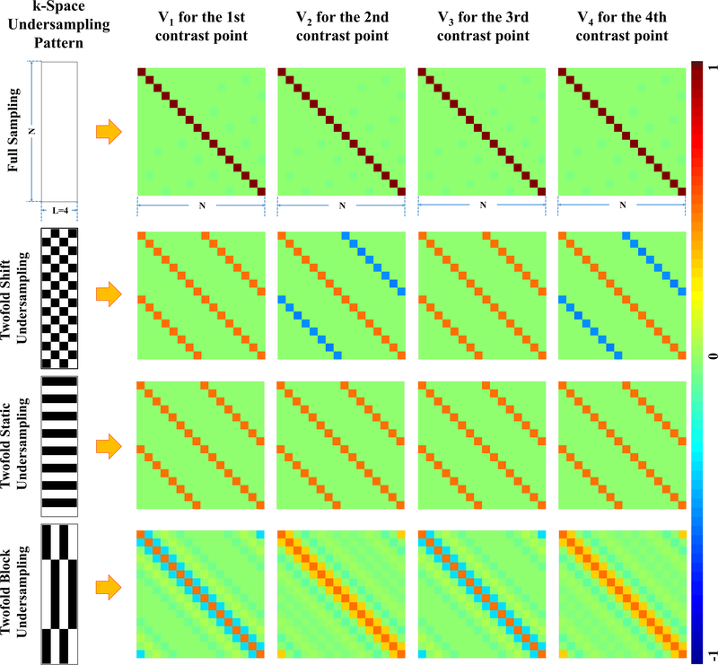
GCFN2 is seldom used in model-based reconstruction literature, since Vl is generally not sparse while the fast Fourier transform in GCFN1 can be rapidly executed. However, Vl is sparse if k-space is uniformly undersampled. In a trivial example, Vl is an identity matrix (Figure 1, row 1) if k-space is fully sampled, enabling fast reconstruction with voxelwise curve-fitting. In another example, if k-space is uniformly undersampled (Figure 1, rows 2 and 3), Vl is a banded matrix, leading to so-called blockwise curve-fitting as introduced below.
Figure 1.
Different k-space undersampling patterns and their Vl matrices. Row 1 shows complete k-space sampling, which leads to an identity matrix for Vl at each contrast point. Row 2 and row 3 show 2-fold shift and static undersampling pattern, respectively, both of which lead to banded Vl matrices that have nonzero values for only 2 voxels at each row. Row 4 shows the block undersampling pattern used by MARTINI, which leads to non-sparse matrices at all contrast points.
Blockwise curve-fitting
When Vl is an identity matrix, each row of Vl corresponds to a single unique voxel. As a result, GCFN2 can be minimized row by row with voxelwise curve-fitting:
| (6) |
where VCFN represents voxelwise cost function. The voxelwise curve-fitting leads to a much faster reconstruction than minimizing either global cost function (Equation 2 or 5), due to the large variable size involved in the latter approach. On the other hand, when Vl is a banded matrix, each row of Vl corresponds to a unique block of voxels, which uniformly span the field of view (FOV) (Figure 1, rows 2 and 3). In this case, GCFN2 can still be minimized row by row, but each row forms a blockwise curve-fitting problem, where the original signal at each voxel in the block is linearly combined to generate an aliased signal. The size of each block equals the undersampling rate (e.g. R=2), which is usually much smaller than the image size, and thus allows for faster reconstruction.
Mathematically, the block for the nth voxel under R-fold undersampling rate can be represented by a vector of length R, as shown below:
| (7) |
where we made a trivial assumption that R divides N (image size). Let represents parameters in the n th block, the sensitivity matrix of the nth block, the blockwise cost function (BCFN) is given by:
| (8) |
where is a vector representing the coefficient of each voxel and formed by the nonzero values of matrix Vl in the first row (or equivalently any other row since Vl is a convolution matrix):
| (9) |
where [·]r and represent the corresponding elements in a vector or matrix. Note that for each n in Equation 8, parameters of all R voxels in the block are estimated. When R=1, BCFN relaxes to VCFN, demonstrating that voxelwise curve-fitting is a special case of blockwise curve-fitting.
To summarize, model-based reconstruction can be fulfilled by blockwise curve-fitting only when k-space is uniformly undersampled at each contrast point. Otherwise, Vl is not sparse (Figure 1, row 4), and the reconstruction must be performed over the entire image space, such as in the case of MARTINI (9) or GRAPPATINI (10). Blockwise curve-fitting enables faster reconstruction. However, when blockwise curve-fitting is used, the undersampling pattern across different contrasts has a strong influence on the accuracy and precision of the estimation result, as discussed below.
Shift undersampling vs static undersampling
The contrast dimension in parametric mapping grants freedom in choosing undersampling patterns. Shift undersampling refers to continuous shifting of the k-space undersampling pattern along the phase-encoding direction at each contrast point (Figure 1, row 2). Static undersampling refers to an unchanged undersampling pattern at every contrast point (Figure 1, row 3). Note that both are uniform undersampling strategies. The static undersampling leads to the following Wl coefficient vector in the blockwise curve-fitting:
| (10) |
To demonstrate the disadvantage of , we use an example of 2-fold accelerated T1 mapping, which has the following BCFN (from Equation 8):
| (11) |
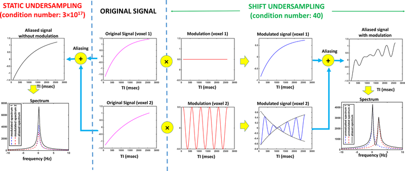
where , , and are parameters at the first voxel in the block, and , and are parameters at the second voxel. Equation 11 suggests that the net effect of on the two aliasing T1-relaxation signals, after ignoring the coil sensitivity, is to directly combine them into the aliased signal. In the contrast-frequency domain, the spectrum of the two T1-relaxation signals are completely aliased, as shown in the Figure 2 (left side). Fitting such a multi-exponential model to noisy data is a well-known ill-conditioned problem (33,34).
Figure 2.
Comparison between shift undersampling and static undersampling. The central panel shows the original T1-relaxation signals at the two aliasing voxels. With static undersampling (left panel), the two signals are directly combined, leading to a complete overlapping between their spectra. The associated inverse problem is severely ill-conditioned with a condition number of 3×10¹⁷. With shift undersampling (right panel), each signal is firstly multiplied by a modulating function with a unique modulation frequency, yielding a smooth signal in the first voxel and an oscillating signal in the second voxel. The two modulated signals are then combined, resulting in a spectrum with two separate spectral peaks, suggesting less spectral overlapping. The associated inverse problem is well-conditioned, with a condition number of 40.
On the other hand, based on the work of UNFOLD (29), TSENSE (30), and KT-BLAST (31), we know that shift undersampling creates a frequency modulation for each aliasing T1-relaxation signal. Mathematically, the frequency modulation is generated by the Wl vector:
| (12) |
The corresponding BCFN for 2-fold accelerated T1 mapping is
| (13) |
Notice the different modulation frequency for the second voxel in the block. In the contrast-frequency domain, the net effect of is to shift the spectrum of each T1-relaxation signal to a unique frequency position, so that each spectrum is distinguishable even after the aliasing (Figure 2, right side). Since the shape of each individual spectrum contains information about the underlying parameters, such as the relaxation rate, a better preservation of the spectrum leads to better accuracy in the reconstruction. From the view of linear algebra, this means a better conditioned inverse problem. In fact, the condition number for the simulation used in Figure 2 was 40 for shift undersampling, which is very reasonable, and 3×10¹⁷ for static undersampling, which suggests severe ill-conditioning.
Nested shift undersampling for SUPER-SENSE (nSUPER-SENSE)
SUPER-SENSE is the combination of SUPER and SENSE to further improve the acceleration rate. SUPER-SENSE solves the same blockwise cost function in Equation 8. However, for a higher undersampling rate (R ≥ 4), there are two basic shift undersampling strategies for SUPER-SENSE. On one hand, the ordinary shift undersampling pattern described by Equation 12 can be used (e.g. at R=4, sampling lines #1, #5, #9 for the first contrast point, and then #2, #6, #10 for the second, and so on and so forth). On the other hand, the shift undersampling pattern can be nested within a static undersampling pattern, such as using sampling lines #1, #5, #9 at odd contrast points and #3, #7, #11 at even contrast points (shift undersampling within the odd lines only). Intuitively, this nested pattern has an advantage, in that a lower shift-undersampling rate can be used, providing a wider spread of modulation frequencies in the contrast-frequency domain. This can be confirmed from the Wl vector of the nested shift undersampling:
| (14) |
where R1 is the acceleration factor for the static-undersampling component, R2 is the acceleration factor for the shift-undersampling component, and 0 ≤ r < R1R2 = R. Since R2 < R, the modulation frequency of nested shift undersampling is greater than of ordinary shift undersampling.
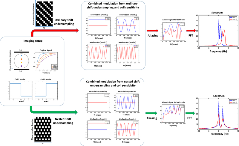
Figure 3 demonstrates this advantage by comparing SUPER-SENSE based on nested shift undersampling (nSUPER-SENSE) to that based on ordinary shift undersampling (oSUPER-SENSE) for 4-fold T1 mapping acceleration. For better demonstration, we assume each coil has a step-function profile and thus only measures signal from the two proximal voxels. The resultant BCFN of each coil for nSUPER-SENSE is:
| (15) |
Figure 3.
Comparison of ordinary and nested shift undersampling for 4-fold SUPER-SENSE. Two coils were simulated, each with a step-function profile. With ordinary shift undersampling (top), each voxel has a unique modulation frequency. With nested shift undersampling (bottom), there is no frequency modulation between voxels half-FOV apart, but these voxels are measured by different coils. On the other hand, nested shift undersampling leads to a spectral difference twice as large as that with ordinary shift undersampling, between voxels ¼-FOV apart (double-headed arrows). This leads to reduced overlapping between these voxels compared to ordinary shift undersampling.
Notice that the modulation frequencies are 0 and for the two aliasing voxels measured by each coil. On the other hand, the BCFN of each coil for oSUPER-SENSE is:
| (16) |
Note that the modulation frequency of the two aliasing voxels differs by only (half of that with nested shift undersampling), increasing spectral aliasing and causing poorer conditioning. Since coil sensitivity generally is more similar for proximal voxels, nSUPER-SENSE works better on compensating for the limitation of parallel imaging by having a stronger modulation for proximal voxels than oSUPER-SENSE. This advantage is also demonstrated with simulations and in vivo data.
Optimization
The optimization of blockwise curve-fitting should not be different from that of voxelwise curve-fitting, since the latter is simply a special case of the former for R=1. One of the most common methods for voxelwise curve-fitting in parametric mapping is Levenberg-Marquardt (1,6,35). In this work, we used a slightly modified Levenberg-Marquardt method for T1-mapping, to restrict each parameter in a physiologically meaningful bound. However, any nonlinear optimization algorithm, such as conjugate gradients should suffice to minimize the blockwise cost function. Details about the proposed Levenberg-Marquadrt algorithm can be found in the Supporting Information due to space limitation.
D-factor
The g-factor, firstly introduced in SENSE (7) and further developed in other works (36,37), is important for quantifying parallel-imaging-induced noise amplification. In this work, we used the same principle to derive the so-called d-factor to quantify the parametric noise amplification due to acceleration. Following the principle underlying SENSE noise amplification, the amplification of parametric noise, represented by standard deviation of the parameter, due to any acceleration is a multiplication of two factors:
| (17) |
where xnj is the jth fitting parameter at the nth voxel, SDR(xnj) is the standard deviation of xnj estimated with R-fold acceleration, SD1(xnj) is the standard deviation of xnj estimated without any acceleration, is a ubiquitous factor that represents a global increase of noise due to the reduced imaging time, and dR(xnj) is the so-called dynamics-factor, or d-factor, which represents the spatially heterogeneous increase of noise due to ill-conditioning of the model-based reconstruction. Like the g-factor in parallel imaging, d-factor should be greater than 1 for any acceleration solely based on model-based reconstruction.
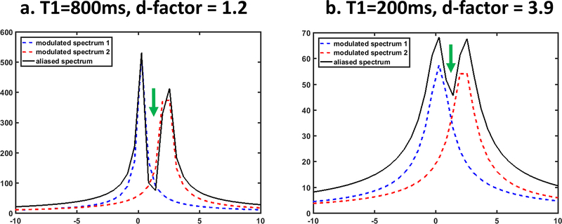
D-factor was named as such because signal dynamics is the main factor affecting the spatial heterogeneity of d-factor, just like the impact of coil geometry on spatial heterogeneity of g-factor. As Figure 4 shows, if a signal grows too fast, the spectrum of each signal would be wider, which causes increased overlapping between aliasing spectra, leading to elevation of d-factors. Since the parameter, such as T1 or T2, is spatially varying, the d-factor is also spatially varying. Other factors, such as density of contrast points and k-space undersampling pattern, also affect the value of d-factor, but in a more spatially uniform fashion (i.e. changing spectral width uniformly). Finally, when parallel imaging is used in model-based reconstruction, g-factor itself also affects the value of d-factor.
Figure 4.
Illustration of the impact of signal dynamics on d-factor, using 2-fold SUPER T1-mapping acceleration. The d-factor is 1.2 when both aliasing signals have T1 of 800ms, and rises to 3.9 when T1 is 200ms. When T1 is reduced, the signal grows faster, resulting in a wider spectrum, which in turn causes more overlapping (arrows) and elevates the d-factor.
In practical applications, d-factor can be approximately calculated by the Cramer-Rao Lower Bound (CRLB) (38,39), which provides a lower bound (thus an approximation) for the variance of the parameters after reconstruction. A derivation of CRLB-based formulation for quantifying parametric noise was given in Ref. (32). Here, we briefly describe the derivation for the sake of completeness. The first step is to use Equation 1 to derive the Fisher Information matrix, which for a normally distributed data, (E is an identity matrix and σ the noise standard deviation), is given by
| (18) |
where I is the Fisher Information matrix, and the first-order derivative of the nonlinear function with respect to the variable x. By definition, CRLB is given by the inverse of Fisher Information matrix:
| (19) |
where CRLBR(x) is a matrix, which represents the lower bound for the covariance matrix of all parameters under R-fold acceleration. The CRLB for each single parameter xnj is given by the corresponding diagonal element of the CRLB matrix:
| (20) |
More detailed derivation for Equations 19–20 can be found in Ref. (32). Based on these equations, we can estimate the d-factor, which, different from CRLB, accounts for the parametric noise amplification due to acceleration, rather than the noise inherent to the non-accelerated parametric mapping. The CRLB-based estimation of d-factor for xnj is given by
| (21) |
Notice that in the denominator is omitted since it’s an identity matrix when R=1.The formulation above is only used for Cartesian trajectories in this work. However, the formulation can also work for non-Cartesian trajectories by substituting DlF to a nonuniform Fourier encoding matrix (32). Notice that this metric only depends on coil sensitivities (Sm), sampling pattern (Dl), and the parametric regrowth curve , but not on the reconstruction methods.
Methods
Simulations, phantom imaging, and in vivo imaging were conducted to compare several acceleration methods for T1 mapping, including the SENSE-based methods, SUPER, nSUPER-SENSE, oSUPER-SENSE, MARTINI (9), and GRAPPATINI (10). Both MARTINI and GRAPPATINI were reconstructed with conjugate gradients (CG)(40) line-by-line for each line along the phase-encoding direction. This CG algorithm is the same type used in the original work of MARTINI (9) and GRAPPATINI (10). CG was stopped using the same rule as in SUPER or SUPER-SENSE except for a larger number of iterations, due to the larger variable size: a) number of iterations greater than 1000 (SUPER/SUPER-SENSE uses 300), b) , or c) stepsize less than 1×10⁻⁶ of the initial stepsize.
All imaging was performed on a 3T scanner (Siemens Trio, Erlangen, Germany). All the subjects enrolled to the study provided informed written consent prior to the scan. The study was approved by our institutional review board (IRB).
Simulations
A digital phantom with A=1, B=2, and 4 T1s (200ms, 500ms, 1000ms, 1500ms) was used to generate k-space data, with 6 coils and 6 TI values (100ms, 200ms, 500ms, 1000ms, 2000ms, 5000ms). The k-space data was then undersampled for 8 different reconstruction methods, including the standard non-acceleration method (R=1), SUPER (R=2), static undersampling based blockwise curve-fitting (R=2), MARTINI (R=2), SENSE (R=4), oSUPER-SENSE (R=4), nSUPER-SENSE (R=4), and GRAPPATINI (R=4).
Phantom study
Fourteen vials filled with Gadolinium-doped water or a mixed solution of NiCl2 and agar gel with T1 ranging from 200ms to 1500ms were scanned with a 12-channel head coil using 7 repetitions of an inversion recovery turbo spin-echo (IR TSE) sequence, with TI of 100ms, 200ms, 400ms, 800ms, 1600ms, 3200ms, and 6400ms. Other parameters were: FOV = 280mm×140mm, image size = 192×96, TR=7000ms, TE=4.9ms, slice thickness=5mm, echo train length (ETL) = 12, and bandwidth = 789Hz/pixel. Eight reconstruction methods were performed: the standard non-acceleration method (R=1), SENSE (R=2), SUPER (R=2), MARTINI (R=2), SENSE (R=4), nSUPER-SENSE (R=4), oSUPER-SENSE (R=4), and GRAPPATINI (R=4). Coil mapping was performed using the TSE image at TI=6400ms with the method in (41).
Brain T1 mapping
Brain T1 mapping was performed in 5 healthy subjects (4 male, age 26±3) with a 12-channel quadrature head coil and 8 continuously applied IR TSE with TI of 250ms, 500ms, 750ms, 1000ms, 1500ms, 2000ms, 3500ms, and 5000ms. Other parameters were: TR=5200ms, ETL=16, FOV=240mm×240mm, acquisition matrix size=256×128, slice thickness=4mm, and bandwidth=789 Hz/pixel. Seven reconstruction methods were performed: the standard non-acceleration method (R=1), SENSE (R=2), SUPER (R=2), MARTINI (R=2), nSUPER-SENSE (R=4), oSUPER-SENSE (R=4), and GRAPPATINI (R=4). White matter, gray matter, and cerebrospinal fluid (CSF) ROIs were segmented on the gold standard T1 map using thresholding, with T1 in [580ms, 1080ms] classified as the white matter, [1080ms, 1580ms] as gray matter, and [3000ms, 6000ms] classified as CSF (42).
High-resolution cardiac T1 mapping
Parametric mapping, such as T1 or T2 mapping, has been extensively used in cardiac MR for clinical assessment of myocardial fibrosis (6,43) or edema (1). The standard MOLLI T1 mapping (6) is based on cardiac gated single-shot acquisition and 2-fold parallel imaging, but suffers from low spatial resolution. K-space undersampling cannot be used to reduce the total imaging time, which is only determined by the number of TIs collected, but can be used to improve image resolution of the single-shots acquisitions in each heartbeat. Here we aim to demonstrate the capability of SUPER-SENSE for high-resolution single-breath-hold cardiac T1 mapping in vivo.
MOLLI was performed in 8 healthy subjects (3 male, age 33±7) with a 24-channel spine coil and 18-channel body coil in a short-axis mid-ventricular slice. The standard MOLLI (6) sequence (17 heartbeats, 3(3)3(3)5 scheme, TI=100ms, 200ms, and 350ms) was modified to enable SUPER-SENSE acquisition with a higher spatial resolution. T1 mapping was firstly performed with the standard MOLLI (resolution=1.9mm×2.5mm, 2-fold SENSE), and then 4-fold SUPER-SENSE MOLLI (resolution=1.4mm×1.4mm). Other parameters were: FOV= 360mm×270mm, slice thickness=8mm, bandwidth=1495 Hz/pixel, TR=2.5ms, and flip angle=40°. The central 24 k-space lines were sampled for coil mapping (41). ROIs were drawn in the myocardial and blood pool.
Evaluation metrics
All reconstruction was performed offline with Matlab (v2014b, Mathworks, Natick, MA). In simulations, phantom T1 mapping, and brain T1 mapping, normalized root-mean-square error (NRMSE), defined by l2-norm of the difference between solution and the gold standard divided by the l2-norm of the gold standard, was calculated for each method. The d-factor map was calculated and matched to the T1-difference map for each acceleration method. The d-factor map also provided a metric for characterizing and comparing the noise property of each method.
Computational efficiency was evaluated using computational time per voxel (TPV), since TPV does not vary with spatial resolution as in the case of total computational time. For all blockwise curve-fitting methods, TPV was the computational time per optimization divided by the acceleration rate. For MARTINI or GRAPPATINI, TPV was the computational time per optimization divided by the number of voxels along the phase-encoding direction.
For in vivo studies, NRMSE (if available), mean T1 in each ROI, the average d-factor over the cerebral cortex region or the heart, and TPV were statistically compared between different methods via Student’s t-test. A p-value less than 0.05 was considered statistically significant.
Results
Simulations
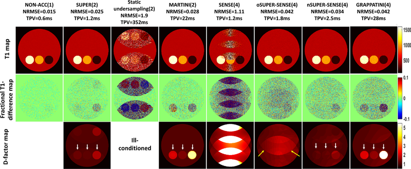
Figures 5 shows the reconstruction results for the simulated phantom. All methods led to good visual quality except static undersampling (column 3) and 4-fold SENSE (column 5), due to severe ill-conditioning and large g-factors, respectively. oSUPER-SENSE (column 6) was noisier than nSUPER-SENSE (column 7) due to a higher d-factor especially around the image center. The d-factor map of oSUPER-SENSE shows mainly a 4-fold aliasing pattern (yellow arrows), while that of nSUPER-SENSE shows mainly a 2-fold aliasing pattern, consistent with our theoretical anticipation. Furthermore, SUPER (column 2) and nSUPER-SENSE provided higher precision in those small bottles (white arrows) than MARTINI (column 4) and GRAPPATINI (last column), respectively, also due to elevated d-factor in the latter cases. The d-factor maps excellently matched the T1-difference map for all methods. The fact that all 4-fold acceleration methods led to noisier reconstruction than 2-fold acceleration methods is partly due to the global noise amplification in Equation 17, which equals the square root of the acceleration rate.
Figure 5.
Simulation comparing standard non-acceleration T1 mappng (R=1), SUPER (R=2), static undersampling based T1 mapping (R=2), MARTINI (R=2), SENSE-based T1 mapping (R=4), oSUPER-SENSE (R=4), nSUPER-SENSE (R=4), and GRAPPATINI (R=4). The top, middle, and bottom row shows the reconstructed T1 maps, the fractional T1-difference maps, and the d-factor maps for each method. The d-factor map for the static undersampling based T1 mapping cannot be calculated due to the severe ill-conditioning, NRMSE and TPV were noted under each method’s name. Yellow arrows point to the elevation of d-factor due to 4-fold aliasing in oSUPER-SENSE. White arrows point to the little bottles, with T1 of 200ms (right), 1000ms (middle), and 1500ms (left), which have a higher d-factor with MARTINI/GRAPPATINI than SUPER/SUPER-SENSE.
Phantom studies
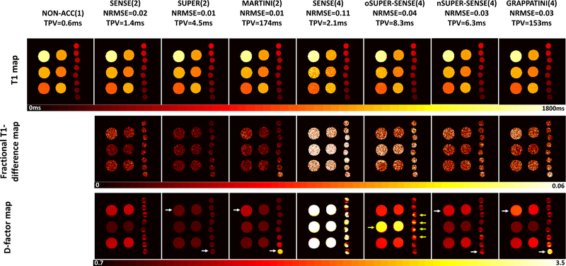
Figure 6 shows the phantom study results, which demonstrated a similar trend as the simulation results. SENSE (columns 2 and 5) led to noisier results compared to all other methods at the same acceleration rate. oSUPER-SENSE (column 6) was much noisier than nSUPER-SENSE (column 7), due to elevated d-factors in the image center (yellow arrows). MARTINI/GRAPPATINI (columns 4 and 8) led to noisier results than SUPER/nSUPER-SENSE (columns 3 and 7) in the vials with an excessively high or low T1 (white arrows). The d-factor maps also excellently matched the T1-difference maps for all methods.
Figure 6.
Phantom T1 mapping comparing standard non-acceleration T1 mappng (R=1), SENSE-based T1 mapping (R=2), SUPER (R=2), MARTINI (R=2), SENSE-based T1 mapping (R=4), oSUPER-SENSE (R=4), nSUPER-SENSE (R=4), and GRAPPATINI (R=4). The top, middle, and bottom row shows the reconstructed T1 maps, the fractional T1-difference maps, and the d-factor maps for each method. NRMSE and TPV were noted under each acceleration method’s name. Yellow arrows point to the elevation of d-factor due to 4-fold aliasing in oSUPER-SENSE. White arrows point to the bottles with the highest (1600ms) and lowest T1 (200ms), which have a higher d-factor with MARTINI/GRAPPATINI than SUPER/SUPER-SENSE.
Brain T1 mapping
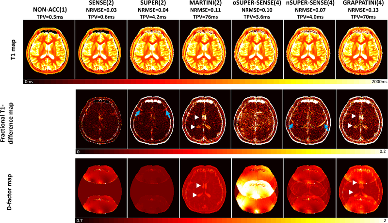
Figure 7 shows the reconstruction results from one healthy subject. Consistent with all previous results, oSUPER-SENSE (column 5) was noisier than nSUPER-SENSE (column 6), with the main elevation of d-factor in the image center, showing a strong 4-fold aliasing pattern. SUPER/nSUPER-SENSE (columns 3 and 6) achieved lower NRMSE than MARTINI/GRAPPATINI (columns 4 and 7). In particular, CSF T1 was more accurately estimated with SUPER/nSUPER-SENSE, due to a lower d-factor in this region (white arrow heads). However, SUPER/nSUPER-SENSE showed mild aliasing artifacts in the image (blue arrows), which were aliased from the interface region between skull and subcutaneous fat, potentially due to partial-voluming between these tissues.
Figure 7.
Brain T1 mapping in one healthy subject. Seven methods were compared: standard non-acceleration T1 mappng (R=1), SENSE-based T1 mapping (R=2), SUPER (R=2), MARTINI (R=2), oSUPER-SENSE (R=4), nSUPER-SENSE (R=4), and GRAPPATINI (R=4). The top, middle, and bottom row shows the reconstructed T1 maps, the fractional T1-difference maps, and the d-factor maps for each method. NRMSE and TPV were noted under each acceleration method’s name. Blue arrows point to the aliasing artifacts in SUPER and SUPER-SENSE due to model inconsistency. White arrow heads point to the increased bias and d-factor in CSF using MARTINI and GRAPPATINI.
Figure 8a shows the ROI-based comparison between each acceleration method and the gold standard, where CSF T1 was severely underestimated with MARTINI and GRAPPATINI. Figure 8b shows statistical comparison of NRMSE, average d-factor, and TPV. On one hand, NRMSE and d-factor were lower comparing SUPER to MARTINI (NRMSE: 0.04±0.02 vs 0.11±0.02, p<0.01; d-factor: 1.01±0.002 vs 1.12±0.004, p<0.001), nSUPER-SENSE to oSUPER-SENSE, and nSUPER-SENSE to GRAPPATINI (NRMSE: 0.07±0.01 vs 0.13±0.03, p=0.02; d-factor: 1.15±0.01 vs 1.20±0.01, p<0.001). On the other hand, TPV was dramatically reduced comparing SUPER to MARTINI (4.6ms±0.2ms vs 79ms±3ms, p<0.001), and nSUPER-SENSE to GRAPPATINI (4.0ms±0.1ms vs 72ms±3ms, p<0.001). The reconstruction of SUPER/nSUPER-SENSE was much faster than MARTINI/GRAPPATINI, and similar to voxelwise curve-fitting on the absolute time scale.
Figure 8.
(a) Plot of the average T1 of white matter (WM) ROI, gray matter (GM) ROI, and CSF ROI over 5 subjects measured by different acceleration methods against the standard non-acceleration T1 mapping. The red arrow points to the large underestimate of CSF T1 with MARTINI and GRAPPATINI. (b) Statistical comparison between different acceleration methods in terms of NRMSE (value multiplied by 500), average d-factor (value multiplied by 50), and computational time per voxel over 5 subjects.
High-resolution cardiac T1 mapping
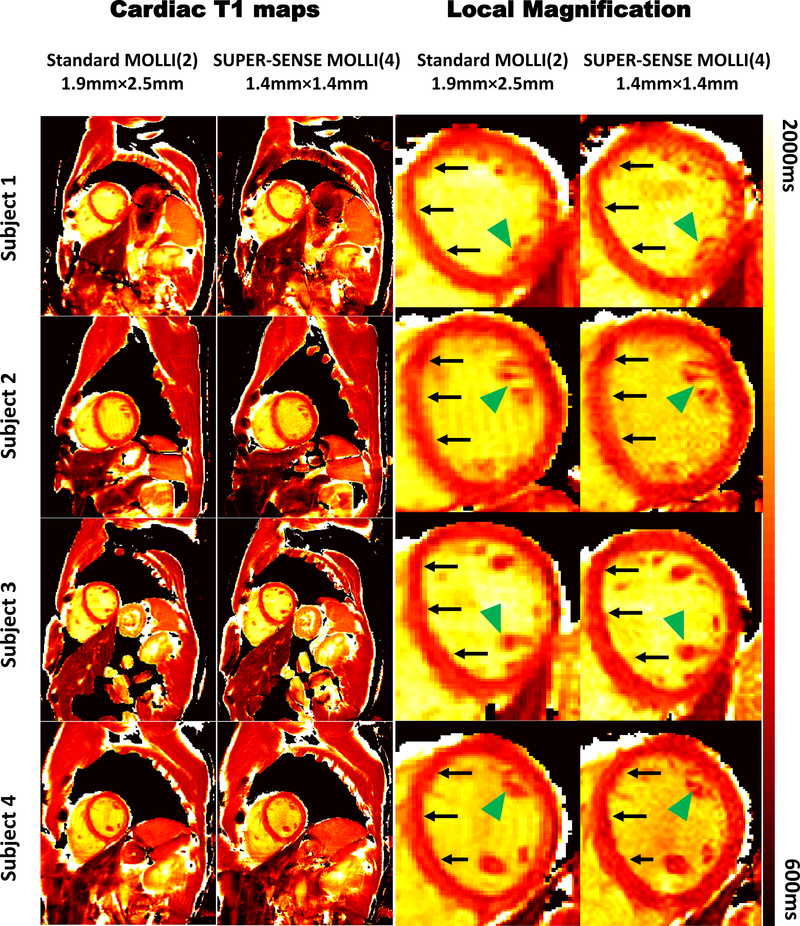
Figure 9 shows the reconstruction result of standard MOLLI and SUPER-SENSE MOLLI in 4 healthy subjects. Both led to excellent image quality under visual inspection. However, the higher resolution of nSUPER-SENSE improved depiction of the septal walls (black arrows), especially at its boundary against the blood pool, and of papillary muscles (green arrow heads), compared to the low-resolution results.
Figure 9.
Representative T1 maps acquired with the standard MOLLI (R=2) and SUPER-SENSE MOLLI (R=4) in 4 healthy subjects. On the right shows the magnified T1 maps around the heart for both methods to demonstrate the improvement of spatial resolution with SUPER-SENSE MOLLI, which leads to better depiction of septal wall (arrows) and papillary muscles (arrow heads).
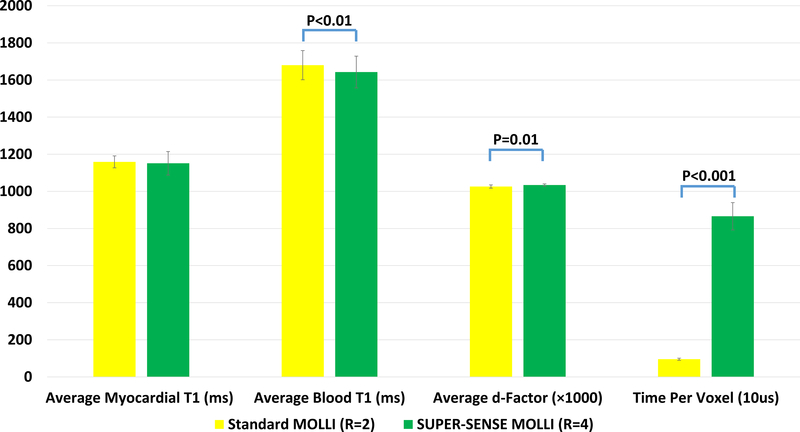
Figure 10 shows the statistical comparison of average myocardial T1, average blood T1, average d- factor in the heart, and average TPV. SUPER-SENSE MOLLI yielded similar myocardial T1 (1151ms±63ms vs 1159±32ms, p=0.6), slightly lower blood T1 (1643ms±86ms vs 1680ms±79ms, p=0.004), slightly larger d-factor (1.034±0.006 vs 1.026±0.008, p=0.01), and longer TPV (8.7ms±0.7ms vs 1.0ms±0.1ms, p<0.001) compared to the standard MOLLI.
Figure 10.
Statistical comparison between standard MOLLI and SUPER-SENSE MOLLI in terms of average myocardial T1, average blood T1, average d-factor (multiplied by 1000), and time per voxel in the unit of 10 microseconds.
Reconstruction time comparison
The reconstruction time quantified by TPV of voxelwise curve-fitting, SUPER, SUPER-SENSE, MARTINI, and GRAPPATINI for all the experiments is collectively shown in Supporting Information Table S1. The speed-up of SUPER relative to MARTINI, and SUPER-SENSE relative to GRAPPATINI, is shown in Supporting Information Table S2. Overall, SUPER and SUPER-SENSE achieved a speed-up around 20 relative to MARTINI and GRAPPATINI, respectively.
Discussions and Conclusion
In this work, we have proposed a novel model-based acceleration method for parametric mapping using shift undersampling. We have demonstrated its utility in accelerated brain T1-mapping, and cardiac T1 mapping with increased spatial resolution. The value of shift undersampling lies in its capability to separate different aliasing spectra, and further to enable blockwise curve-fitting, which allows for fast reconstruction due to greatly reduced computational burden. This is a major innovation of SUPER, since many model-based methods, including MARTINI and GRAPPATINI, are based on iterative algorithms that update the parametric maps on the entire image domain. SUPER and SUPER-SENSE thus provide a fast model-based reconstruction approach that is very suitable for clinical utilization.
Another contribution of the work was to propose the concept of d-factor for quantifying parametric noise amplification due to acceleration. This concept enriches the theory of acceleration-induced noise amplification in MRI, which was originally developed for parallel imaging (g-factor) only. Using d-factor, we demonstrated the advantages of SUPER and nSUPER-SENSE over alternative undersampling patterns, including MARTINI and GRAPPATINI, on minimizing the noise amplification. The difference between d-factor and the CRLB formulation developed in the previous work (32), is that d-factor quantifies the amplification of noise, while CRLB quantifies noise itself, which is a combined effect of many factors such as magnetic field strength, coil loading, voxel size, and acceleration rate. D-factor, however, separates the impact of acceleration from all the other SNR-related factors, providing specific information about the compromise between amplification of parametric noise and the acceleration.
A prior study (9) found less aliasing artifacts using MARTINI vs. a SUPER-like acquisition (but with traditional reconstruction) for brain T2 mapping in the presence of partial-voluming. We also found aliasing artifacts with SUPER in our brain study, probably also due to partial-voluming. However, we have demonstrated with our experiments that SUPER/SUPER-SENSE achieves a lower noise amplification than MARTINI/GRAPPATINI, which is probably attributable to the k-space undersampling difference, in that SUPER/SUPER-SENSE samples central k-space twice as often as MARTINI/GRAPPATINI. This difference is especially significant for extreme T1 values, which have a higher requirement on sufficient sampling of the contrast domain to cover the signal dynamics. In addition, the prior works did not utilize blockwise curve-fitting for SUPER reconstruction, which is proposed in this work.
The aliasing artifacts in SUPER can be generated from factors such as motion, partial volume, and other acquisition imperfections, such as J-coupling (44) or combined T1/T2 contrast (45), which all cause imperfect modeling. The impact of these other sources of parametric mapping is not addressed in this work. However, a potential method for suppressing this artifact is to use data-driven models, such as those based on principal component analysis (18,25,28), which is under our current investigation. In this study, we did not compare SUPER with more advanced regularization-based acceleration methods (18–21,24–28), which rely on sparsity and an incoherent sampling pattern. The uniform sampling strategy of SUPER enables the very fast reconstruction, and has other advantages of a Cartesian acquisition, such as its insensitivity to gradient system imperfections (46), but also makes SUPER potentially incompatible with compressed sensing.
In conclusion, we have proposed a novel technique for parametric mapping with very fast reconstruction, and a tool for evaluating the noise amplification due to model-based acceleration in parametric mapping. The technique utilizes so-called shift undersampling pattern in k-space and blockwise curve-fitting in the reconstruction, which has a comparable reconstruction time to the conventional voxelwise curve-fitting. The concept of d-factor is fully integrable with the conventional g-factor, to characterize spatially heterogeneous noise amplification in parametric mapping. These tools may greatly improve the clinical appeal of parametric mapping.
Supplementary Material
Acknowledgments
Funding: This work was partially supported by grants from the NIH R01HL122560
Reference
- 1.Giri S, Chung YC, Merchant A, Mihai G, Rajagopalan S, Raman SV, Simonetti OP. T2 quantification for improved detection of myocardial edema. J Cardiovasc Magn Reson 2009;11:56. [DOI] [PMC free article] [PubMed] [Google Scholar]
- 2.Deoni SC, Peters TM, Rutt BK. High-resolution T1 and T2 mapping of the brain in a clinically acceptable time with DESPOT1 and DESPOT2. Magn Reson Med 2005;53(1):237–241. [DOI] [PubMed] [Google Scholar]
- 3.Akcakaya M, Basha TA, Weingartner S, Roujol S, Berg S, Nezafat R. Improved quantitative myocardial T2 mapping: Impact of the fitting model. Magn Reson Med 2014. [DOI] [PMC free article] [PubMed] [Google Scholar]
- 4.Chow K, Flewitt JA, Green JD, Pagano JJ, Friedrich MG, Thompson RB. Saturation recovery single-shot acquisition (SASHA) for myocardial T(1) mapping. Magn Reson Med 2014;71(6):2082–2095. [DOI] [PubMed] [Google Scholar]
- 5.Weingartner S, Akcakaya M, Basha T, Kissinger KV, Goddu B, Berg S, Manning WJ, Nezafat R. Combined saturation/inversion recovery sequences for improved evaluation of scar and diffuse fibrosis in patients with arrhythmia or heart rate variability. Magn Reson Med 2014;71(3):1024–1034. [DOI] [PubMed] [Google Scholar]
- 6.Messroghli DR, Radjenovic A, Kozerke S, Higgins DM, Sivananthan MU, Ridgway JP. Modified Look-Locker inversion recovery (MOLLI) for high-resolution T1 mapping of the heart. Magn Reson Med 2004;52(1):141–146. [DOI] [PubMed] [Google Scholar]
- 7.Pruessmann KP, Weiger M, Scheidegger MB, Boesiger P. SENSE: sensitivity encoding for fast MRI. Magn Reson Med 1999;42(5):952–962. [PubMed] [Google Scholar]
- 8.Griswold MA, Jakob PM, Heidemann RM, Nittka M, Jellus V, Wang J, Kiefer B, Haase A. Generalized autocalibrating partially parallel acquisitions (GRAPPA). Magn Reson Med 2002;47(6):1202–1210. [DOI] [PubMed] [Google Scholar]
- 9.Sumpf TJ, Uecker M, Boretius S, Frahm J. Model-based nonlinear inverse reconstruction for T2 mapping using highly undersampled spin-echo MRI. J Magn Reson Imaging 2011;34(2):420–428. [DOI] [PubMed] [Google Scholar]
- 10.Hilbert T, Sumpf TJ, Weiland E, Frahm J, Thiran JP, Meuli R, Kober T, Krueger G. Accelerated T2 mapping combining parallel MRI and model-based reconstruction: GRAPPATINI. J Magn Reson Imaging 2018. [DOI] [PubMed] [Google Scholar]
- 11.Knopp T, Eggers H, Dahnke H, Prestin J, Senegas J. Iterative off-resonance and signal decay estimation and correction for multi-echo MRI. IEEE Trans Med Imaging 2009;28(3):394–404. [DOI] [PubMed] [Google Scholar]
- 12.Tran-Gia J, Stab D, Wech T, Hahn D, Kostler H. Model-based Acceleration of Parameter mapping (MAP) for saturation prepared radially acquired data. Magn Reson Med 2013;70(6):1524–1534. [DOI] [PubMed] [Google Scholar]
- 13.Zhao L, Feng X, Meyer CH. Direct and accelerated parameter mapping using the unscented Kalman filter. Magn Reson Med 2016;75(5):1989–1999. [DOI] [PMC free article] [PubMed] [Google Scholar]
- 14.Ma D, Gulani V, Seiberlich N, Liu K, Sunshine JL, Duerk JL, Griswold MA. Magnetic resonance fingerprinting. Nature 2013;495(7440):187–192. [DOI] [PMC free article] [PubMed] [Google Scholar]
- 15.Block KT, Uecker M, Frahm J. Model-based iterative reconstruction for radial fast spin-echo MRI. IEEE Trans Med Imaging 2009;28(11):1759–1769. [DOI] [PubMed] [Google Scholar]
- 16.Hu C, Reeves SJ. Trust Region Methods for the Estimation of a Complex Exponential Decay Model in MRI With a Single-Shot or Multi-Shot Trajectory. IEEE Transactions on Image Processing 2015;24(11):3694–3706. [DOI] [PubMed] [Google Scholar]
- 17.Hu C, Reeves S, Peters DC, Twieg D. An Efficient Reconstruction Algorithm Based on the Alternating Direction Method of Multipliers for Joint Estimation of R2* and Off-Resonance in fMRI. IEEE transactions on medical imaging 2017;36(6):1326–1336. [DOI] [PubMed] [Google Scholar]
- 18.Zhang T, Pauly JM, Levesque IR. Accelerating parameter mapping with a locally low rank constraint. Magn Reson Med 2015;73(2):655–661. [DOI] [PMC free article] [PubMed] [Google Scholar]
- 19.Lee D, Jin KH, Kim EY, Park SH, Ye JC. Acceleration of MR parameter mapping using annihilating filter-based low rank hankel matrix (ALOHA). Magn Reson Med 2016;76(6):1848–1864. [DOI] [PubMed] [Google Scholar]
- 20.Peng X, Ying L, Liu Y, Yuan J, Liu X, Liang D. Accelerated exponential parameterization of T2 relaxation with model-driven low rank and sparsity priors (MORASA). Magn Reson Med 2016;76(6):1865–1878. [DOI] [PubMed] [Google Scholar]
- 21.Zhao B, Lu W, Hitchens TK, Lam F, Ho C, Liang ZP. Accelerated MR parameter mapping with low-rank and sparsity constraints. Magn Reson Med 2015;74(2):489–498. [DOI] [PMC free article] [PubMed] [Google Scholar]
- 22.Mandava S, Keerthivasan MB, Li Z, Martin DR, Altbach MI, Bilgin A. Accelerated MR parameter mapping with a union of local subspaces constraint. Magnetic Resonance in Medicine 2018;80(6):2744–2758. [DOI] [PMC free article] [PubMed] [Google Scholar]
- 23.Velikina JV, Samsonov AA. Reconstruction of dynamic image series from undersampled MRI data using data-driven model consistency condition (MOCCO). Magn Reson Med 2015;74(5):1279–1290. [DOI] [PMC free article] [PubMed] [Google Scholar]
- 24.Doneva M, Bornert P, Eggers H, Stehning C, Senegas J, Mertins A. Compressed sensing reconstruction for magnetic resonance parameter mapping. Magn Reson Med 2010;64(4):1114–1120. [DOI] [PubMed] [Google Scholar]
- 25.Huang C, Graff CG, Clarkson EW, Bilgin A, Altbach MI. T2 mapping from highly undersampled data by reconstruction of principal component coefficient maps using compressed sensing. Magn Reson Med 2012;67(5):1355–1366. [DOI] [PMC free article] [PubMed] [Google Scholar]
- 26.Velikina JV, Alexander AL, Samsonov A. Accelerating MR parameter mapping using sparsity-promoting regularization in parametric dimension. Magn Reson Med 2013;70(5):1263–1273. [DOI] [PMC free article] [PubMed] [Google Scholar]
- 27.Majumdar A, Ward RK. Accelerating multi-echo T2 weighted MR imaging: analysis prior group-sparse optimization. J Magn Reson 2011;210(1):90–97. [DOI] [PubMed] [Google Scholar]
- 28.Feng L, Otazo R, Jung H, Jensen JH, Ye JC, Sodickson DK, Kim D. Accelerated cardiac T2 mapping using breath-hold multiecho fast spin-echo pulse sequence with k-t FOCUSS. Magn Reson Med 2011;65(6):1661–1669. [DOI] [PMC free article] [PubMed] [Google Scholar]
- 29.Madore B, Glover GH, Pelc NJ. Unaliasing by fourier-encoding the overlaps using the temporal dimension (UNFOLD), applied to cardiac imaging and fMRI. Magn Reson Med 1999;42(5):813–828. [DOI] [PubMed] [Google Scholar]
- 30.Kellman P, Epstein FH, McVeigh ER. Adaptive sensitivity encoding incorporating temporal filtering (TSENSE). Magn Reson Med 2001;45(5):846–852. [DOI] [PubMed] [Google Scholar]
- 31.Tsao J, Boesiger P, Pruessmann KP. k-t BLAST and k-t SENSE: dynamic MRI with high frame rate exploiting spatiotemporal correlations. Magn Reson Med 2003;50(5):1031–1042. [DOI] [PubMed] [Google Scholar]
- 32.Zhao B, Lam F, Liang ZP. Model-based MR parameter mapping with sparsity constraints: parameter estimation and performance bounds. IEEE Trans Med Imaging 2014;33(9):1832–1844. [DOI] [PMC free article] [PubMed] [Google Scholar]
- 33.Yeramian E, Claverie P. Analysis of multiexponential functions without a hypothesis as to the number of components. Nature 1987;326(6109):169. [Google Scholar]
- 34.Martin JL, Maconochie DJ, Knight DE. A novel use of differential equations to fit exponential functions to experimental data. Journal of neuroscience methods 1994;51(2):135–146. [DOI] [PubMed] [Google Scholar]
- 35.Moré JJ. The Levenberg-Marquardt algorithm: implementation and theory Numerical analysis: Springer; 1978. p 105–116. [Google Scholar]
- 36.Robson PM, Grant AK, Madhuranthakam AJ, Lattanzi R, Sodickson DK, McKenzie CA. Comprehensive Quantification of Signal-to-Noise Ratio and g-Factor for Image-Based and k-Space-Based Parallel Imaging Reconstructions. Magnetic resonance in medicine : official journal of the Society of Magnetic Resonance in Medicine / Society of Magnetic Resonance in Medicine 2008;60(4):895–907. [DOI] [PMC free article] [PubMed] [Google Scholar]
- 37.Breuer FA, Kannengiesser SA, Blaimer M, Seiberlich N, Jakob PM, Griswold MA. General formulation for quantitative G-factor calculation in GRAPPA reconstructions. Magn Reson Med 2009;62(3):739–746. [DOI] [PubMed] [Google Scholar]
- 38.Cramér H Mathematical methods of statistics (PMS-9): Princeton university press; 2016. [Google Scholar]
- 39.Rao CR. Information and the accuracy attainable in the estimation of statistical parameters Breakthroughs in statistics: Springer; 1992. p 235–247. [Google Scholar]
- 40.Hager WW, Zhang H. A new conjugate gradient method with guaranteed descent and an efficient line search. SIAM Journal on optimization 2005;16(1):170–192. [Google Scholar]
- 41.McKenzie CA, Yeh EN, Ohliger MA, Price MD, Sodickson DK. Self-calibrating parallel imaging with automatic coil sensitivity extraction. Magn Reson Med 2002;47(3):529–538. [DOI] [PubMed] [Google Scholar]
- 42.Wansapura JP, Holland SK, Dunn RS, Ball WS Jr, NMR relaxation times in the human brain at 3.0 tesla. J Magn Reson Imaging 1999;9(4):531–538. [DOI] [PubMed] [Google Scholar]
- 43.Moon JC, Messroghli DR, Kellman P, Piechnik SK, Robson MD, Ugander M, Gatehouse PD, Arai AE, Friedrich MG, Neubauer S, et al. Myocardial T1 mapping and extracellular volume quantification: a Society for Cardiovascular Magnetic Resonance (SCMR) and CMR Working Group of the European Society of Cardiology consensus statement. J Cardiovasc Magn Reson 2013;15:92. [DOI] [PMC free article] [PubMed] [Google Scholar]
- 44.Henkelman RM, Hardy PA, Bishop JE, Poon CS, Plewes DB. Why fat is bright in RARE and fast spin-echo imaging. J Magn Reson Imaging 1992;2(5):533–540. [DOI] [PubMed] [Google Scholar]
- 45.Kellman P, Hansen MS. T1-mapping in the heart: accuracy and precision. J Cardiovasc Magn Reson 2014;16:2. [DOI] [PMC free article] [PubMed] [Google Scholar]
- 46.Peters DC, Derbyshire JA, McVeigh ER. Centering the projection reconstruction trajectory: reducing gradient delay errors. Magnetic resonance in medicine 2003;50(1):1–6. [DOI] [PMC free article] [PubMed] [Google Scholar]
Associated Data
This section collects any data citations, data availability statements, or supplementary materials included in this article.


