Dynamic Human Environmental Exposome Revealed by Longitudinal Personal Monitoring

Chao Jiang; Xin Wang; Xiyan Li; Jingga Inlora; Ting Wang; Qing Liu; Michael Snyder

doi:10.1016/j.cell.2018.08.060

. Author manuscript; available in PMC: 2019 Sep 20.

Published in final edited form as: Cell. 2018 Sep 20;175(1):277–291.e31. doi: 10.1016/j.cell.2018.08.060

Dynamic Human Environmental Exposome Revealed by Longitudinal Personal Monitoring

Chao Jiang ^1,^2,^3,⁴, Xin Wang ^1,^3,⁴, Xiyan Li ^1,⁴, Jingga Inlora ^1,⁴, Ting Wang ^1,⁴, Qing Liu ¹, Michael Snyder ^1,^2,^3,⁵

PMCID: PMC6472932 NIHMSID: NIHMS1507935 PMID: 30241608

Summary

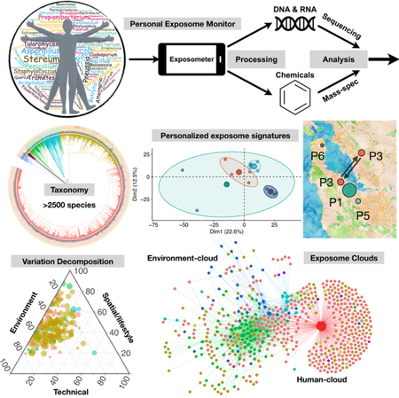
Human health is dependent upon environmental exposures, yet the diversity and variation in exposures is poorly understood. We developed a sensitive method to monitor personal airborne biological and chemical exposures and followed the personal exposomes of 15 individuals for up to 890 days and over 66 distinct geographical locations. We found that individuals are potentially exposed to thousands of pan-domain species and chemical compounds, including insecticides and carcinogens. Personal biological and chemical exposomes are highly dynamic and vary spatial-temporally, even for individuals located in the same general geographical region. Integrated analysis of biological and chemical exposomes revealed strong location-dependent relationships. Finally, construction of an exposome interaction network demonstrated the presence of distinct yet interconnected human- and environment-centric clouds, comprised of interacting ecosystems such as human, flora, pets and arthropods. Overall, we demonstrate that human exposomes are diverse, dynamic, spatiotemporally-driven interaction networks with the potential to impact human health.

Graphical Abstract

graphic file with name nihms-1507935-f0001.jpg

ETOC

Tracking personal exposure to airborne biological and chemical agents enables construction of an interaction network linking individuals, their geographic locations, and environmental factors, which could have broad implications for human health.

Introduction

Human health is greatly impacted by genetics, environmental exposure, and lifestyle. Recently, studies have been performed to understand how genetics and genomic variation can influence our health as well as efforts to understand the molecular mechanisms underlying the effects of lifestyle such as exercise and food ((Laker et al., 2017). These have ushered in an era of personalized medicine (Chen et al., 2012). However, our understanding of human environmental exposures, especially at the personal level, is quite limited. Information about environmental exposures, both biotics (e.g. fungi, pollen, and microbes) and abiotics (e.g. chemicals) can be important for understanding and monitoring numerous diseases such as respiratory diseases, allergy and asthma, chronic inflammatory diseases (Fujimura et al., 2014), and even cancer (Pfeifer, 2010; Tomasetti et al., 2017). Thus, studying environmental exposures will be valuable for understanding human health as well as how humans interact with their environment.

Historically, airborne environmental exposures have been studied by collecting chemical/biological particulates and toxins using immobile sampling stations across distinct geographical locations. These studies have primarily focused on broad detection of air pollutants or simple chemicals, and have revealed useful insights into a variety of human environmental exposures and health (Cao et al., 2014; McCreanor et al., 2007). Studies of personal exposures are much more rare; contact-based chemical exposures using a silicone wristbands have been used to detect personal chemical exposures (O’Connell et al., 2014). Despite these efforts, our understanding of the biotic and abiotic environmental exposures in humans is limited, especially at the personal level. We do not know how vast and dynamic the human biotic and abiotic exposures are and the relative contributions from various spatial-temporal or lifestyle components on the exposure dynamics, nor do we know the relationship among exposure organisms and between the biological and chemical exposures.

In this study, we aimed to establish a comprehensive understanding of human airborne environmental biotic and abiotic exposures, which we collectively refer to as the environmental exposome, or “exposome”. Using a novel approach to systematically interrogate the human airborne exposome for biotics and abiotics we tracked 15 different individuals spatial-temporally, with up to 890 days to provide an extensive personal profiling of the environmental exposome. We find that humans are exposed to thousands of species with great intraspecies diversity and demonstrate that the human exposome is highly dynamic and influenced by spatial/lifestyle and seasonal variables. We describe associations between organisms and chemicals and propose the concept of exposome network based on the extensive interactions among the organisms, which can be partitioned into a stable human-centric cloud and a more dynamic environment-centric cloud. Both the data and approach are expected to be valuable for many scientific fields, including public health, microbiome, environmental science, evolution, and ecology.

Results

A method to capture and decode the personal environmental exposome

We developed a highly sensitive method to monitor the personal exposome using a miniaturized device. A wearable device was modified to actively sample air to capture particulates on a 25 mm sterile filter using optimized filters and sampling methods for the non-biased collection of particulates (Fig. S1A-E and STAR methods). The device also contains a custom 3-D printed zeolite adsorbent cartridge at the end of the airflow that captures large numbers of both hydrophobic and hydrophilic chemical compounds (Fig. S1A). The device is worn on the upper arm or located within a few feet of the subject, and samples air at a steady rate of 0.5L/min (Fig. 1A). Biological agents were detected through optimized isolation and linear amplification protocols followed by deep sequencing (STAR methods). Chemical compounds were extracted by methanol and identified by liquid chromatography coupled mass spectrometry (LC-MS); this method identifies a large variety of hydrophobic and hydrophilic compounds with some limitations (Fig. S1A; STAR methods). Our method is highly sensitive as we are able to detect less than 10 bacterial cells and 200 viral particles, depending on the species (Fig. S1B and C). The device also continuously measures temperature, humidity and particle concentration (Fig. 1B).

We deployed the device on 15 individuals over 66 distinct locations (Fig 1C and D; STAR methods). Three individuals (P1, P2, and P3) were tracked extensively (Fig. 1C): P1 for more than two years (890 days) and 52 locations (201 data points, Fig. 1D and Fig. S1F), P2 for one year and P3 for three months intermittently (Fig. 1C). For P1, sampling was performed such that two filters were typically collected each week (one for weekdays and one for weekends). P1 traveled frequently and each location had a dedicated sampling. Samples from P2 and P3 were collected over longer intervals (1~2 weeks), and sometimes multiple locations. Concurrent chemical exposure sampling was performed on P1 for a period of two months. To visually verify particulates captured by our device, we performed Scanning Electron Microscopy (SEM) on representative filters which revealed diverse biological and inorganic materials; some of these were tentatively assigned based on morphology (Fig. 1E and Fig. S1D) and were consistent with the sequencing results described below.

For each sample, we obtained a median of 62.2M (DNA) and 45.8M (RNA) unique 2×151 bp paired-end reads, resulting in a dataset of 42.9B and 30.4B total reads for DNA and RNA, respectively (Fig. S1G-J), representing the largest personal environmental biological exposure sampling to date. 6.55M (7.4B unique bases) and 1.02M (492M unique bases) contigs were co-assembled from all DNA and RNA reads, respectively. Incorporation of blank filters in each processing batch revealed that contamination effects were very small (Fig. S2A-I; STAR methods).

To gain insights into the biological environmental exposures, we built an extensive reference genome database comprised of more than 40,000 species covering all domains of life (STAR methods). The contigs were queried against the database using discontinuous BLAST and classified using a custom computational analysis pipeline (Fig. S2J and STAR methods). 56.2% of the DNA bases and 64.6% of the RNA bases were classified at the kingdom/subkingdom level using the lowest common ancestor (LCA) algorithm to achieve high specificity. We quantified the relative abundance of individual taxa in Counts Per Million (CPM), by aggregating the number of bases mapped to each contig. We used hyperbolic arcsine (arcsinh) - transformed CPM (aCPM) values for all computational and statistical analyses unless otherwise noted. The fraction and diversity of classified contigs is substantially higher than existing pipelines, which are not adapted to pan-domain detection (Fig. S2K). We confirmed that our methods are reproducible and sensitive (Fig. S2L and Fig. S3A-E). In aggregate, we identified at least 2560 species (including 232 viral species with pan-domain hosts), 1265 genera, and 44 phyla (Fig. 1E-G, Fig. S3F). Individually, P1, P2, and P3 were exposed to 2378, 1357 and 1009 species, for 24, 12, and 3 months of monitoring, respectively, indicating that humans are exposed to more than a thousand biological species within a short period of time.

The human environmental exposome is highly dynamic and diverse.

The analysis of DNA samples revealed highly dynamic exposome profiles in all three individuals (Fig. 2A). Unsupervised clustering of exposome profiles revealed that samples can be grouped into fungi-, plants-, bacteria-, metazoa- dominant groups, with some samples abounding in two or even three kingdoms (Fig. 2B). In contrast, the RNA exposome profiles revealed that bacterial RNA predominates in the majority of the samples (Fig. 2C and D). This is likely due to several reasons: 1. Genomic sizes of eukaryotes can be 1000-fold larger than prokaryotes whereas the sizes of their transcriptomes differ ~10-fold, thus eukaryotic DNA is relatively more abundant in the DNA samples. 2. Some plant and fungi species are probably captured in the form of spore or pollen, rather than active cells (as evidenced by the SEM Fig. 1E and Fig. S1D). Metazoa (animals) are also less prevalent in the RNA exposome, indicating that the metazoan DNA signatures may also come from inactive parts of animals (hair, skin flakes, and brochosomes in Fig. 1E). Despite the differences, the DNA and RNA exposome profiles correlate well at the kingdom and phylum levels; 15 of the top 20 DNA-detected phyla are also found in the top 20 phyla for RNA (Fig. 2E-H). Similar correlating patterns have been reported by studies of human gut microbiome DNA and RNA profiles (Franzosa et al., 2014).

At the phylum level, the top nine phyla in the DNA exposome, including two fungi, four bacterial, and three plant/animal phyla, contribute to the majority of total relative abundance (78.4%) across all samples (Fig. 2E and F). Within the Chordata phylum, we detected contigs for household pets including dogs (0.48% of total aCPM), cats (0.25%) and guinea pigs (0.01%), which were known to co-inhabit with several of the participants (Fig. 2E and F). Interestingly, several other phyla from the metazoan domain were also captured, especially the phylum Rotifera, a group of planktonic and microscopic freshwater/soil organisms able to sustain an asexual life style over millions of years (Flot et al., 2013). P1 was exposed to a very high level of putative rotifers in one sample captured during a holiday period when the subject participated in outdoor sports activities and tree decorations (Fig. S3G and H, last panel). In addition, different human/household-associated arthropods were detected, including several dust, skin and spider mites, as well as mosquitoes, flies, honey bees, and even cockroaches (Fig. S3G and H). Interestingly, we also detected viruses associated with these arthropods, such as those related to the recent honey-bee crisis (Fig. S3G and H), indicating that our method can capture interacting species in the natural environment. Furthermore, our untargeted approach also captured another ubiquitous group of fungi-related eukaryotic organisms, Oomycetes, which are notorious plant pathogens (Fig. S3G and H).

In the RNA exposome, the top ten phyla represent 50.4% of the RNA exposome across all samples (Fig. 2F). It is notable that some species in the top four bacterial phyla, Firmicutes, Proteobacteria, Actinobacteria, and Bacteroidetes are known to associate with humans. Species richness analysis indicated that up to 800 species can be detected during each sampling period and more species were identified in RNA samples compared to their DNA counterparts (Fig. 2I). This is presumably because the RNA exposome detects more bacteria, which have the most species entries in the database. We observed extensive correlation patterns at the phylum and the genus level, indicating potential taxa interactions (Fig. S4A and B).

We also found sequences related to opportunistic and putative pathogens in our DNA and RNA datasets; some share >98% identity to the reference with >90% coverage of the contig (>= 200 bp; Fig. S4C and D). For bacteria and fungi, 15% of samples contained sequences highly homologous to opportunistic pathogens such as Acinetobacter baumannii (Fig. S4C and D), and many mold species such as Penicillum capsulatum (Fig. S4E and F). It is likely that these species are common in the environmental exposome, but only pose threats to immunocompromised individuals. On rare occasions, we detected a few putative pathogenic strains, although no clinical diseases were reported after such exposures (Fig. S4C, red boxes). For viruses, even though our non-targeted approach can detect a variety of respiratory and blood-borne RNA viruses (as few as 200 copies; Fig. S1C and S4G), we did not detect notable respiratory viruses in our samples. It is likely that human RNA viral pathogens are rare in the air environment relative to the other species. In fact, >150 RNA viral species that we found were predominantly associated with plants (Fig. 1G).

We further performed functional analysis of the RNA exposome by querying 1.02M RNA contigs against the NCBI non-redundant protein database, and 66% were identified at the kingdom/subkingdom level (Fig. S5A). Based on the respective top 30 enriched GO annotations (Fig. 2J, and Fig. S5B-D, STAR methods), we found that each taxonomic group displayed both specific and general transcriptional activities. For instance, viral contig sequences were related to capsid, genome integration, and integral to membrane of host cell (Fig. 2J and Fig. S5B-D). To gain more insight into the RNA sequences, we scanned for allergy-related proteins in our transcriptomic data (STAR methods) and identified 31 potential non-food allergen proteins that mostly originated from fungi and plants (Fig. S5E-G). Subsequently, we tracked the relative levels of allergens across different seasons, revealing seasonal patterns of several fungal and plant families (Fig. S5H-K).

In summary, our environmental exposome is highly dynamic and diverse, comprised of thousands of species spanning all domains of life, pre-dominated by a few phyla.

The sources of variation in the human environmental exposome

We investigated the source of variation in the human environmental exposome and focused on the DNA exposome profiles since DNA is more stable than RNA. Conceptually, the exposome can be influenced by at least three major classes of variables: 1. Environmental (Env) such as season, temperature, humidity, wind speed, and particle density. These variables are subject to change over time. 2. Spatial/lifestyle-related (Spa) such as locations, location associated time-insensitive variables such as population density and elevation, and behavior variables. 3. Technical artifacts (Tec) such as batch effects.

To accurately represent the spatial information, we constructed Moran’s Eigenvector Map (MEM) variables to extract broad- and fine-scale spatial structures from the geographic coordinates of each sampling location (Fig. S6A; STAR methods). We divided the 64 collected meta-variables (including the selected MEM variables, complete list in Fig. S6B) into the Env, Spa and Tec groups and carried out forward-selection within each group to select best representative variables. We used partial distance-based redundancy analysis (dbRDA) to decompose the variation in the entire dataset at the genus level (Fig. S6C). Notably, 5 out of 6 MEM variables were selected, indicating that the spatial information is highly relevant (p < 0.05, Fig. S6D). We found that 12.26% of the variation (squared Bray-Curtis distance) in the total DNA exposome can be explained by location/lifestyle-related variables, 9.72% by environmental variables, and only 2.6% of the variation by technical variables that we recorded (Fig. 3A and Fig. S6D and E). In total, 21% of variation can be explained by forward-selected variables (31% can be explained by all variables, Fig. S6E bottom). These numbers are comparable to other ecological studies (Møller and Jennions, 2002).

Fig. 3. — Decomposing the variation in the human environmental exposome. (A) Partial dbRDA variation partitioning analysis. (B) Ternary plots of variation partitioning analysis of highly prevalent genera (detected in >= 100 samples) in different domains of life. Environmental and spatial/lifestyle variables account for more than 80% of the explained variation in at least 75% genera. Each dot represents a genus and the size of the dot corresponds to the total explained variation. Depending on the genera, either environmental (blue) or spatial/lifestyle (dark yellow) variables may play dominant roles, or neither (grey). Contours denote 0.1 to 0.9 confidence intervals. (C) Samples from consecutive time points of P1 in the same location are more similar than those from different locations. (D) Representative differentially abundant genera between the “Campus” (N = 98) and non-”Campus” locations (N = 103). Boxes are color-coded as in Fig. 2A to denote the kingdom/subkingdom of the respective genus. (E) The location of the four individuals (P1, P3, P5, and P6) in the three-week parallel study. The size of dot corresponds to the self-reported activity level of each individual. Arrows indicate commute. (F) PCA analysis of P1, P3, P5 and P6. The bigger colored dots are geometric centers of respective groups. (G) Bray-Curtis distance profiles between samples from the same individual are more similar. (H) Top contributing genera with respect to the PCA analysis in (F). Color indicates relative contribution of each genus. All ellipses are drawn with axes equal to the standard deviation of the data. The Adj. p values are either directly displayed or denoted using the following notations * <0.05, ** < 0.01, *** < 0.001, and **** < 0.0001.

We next dissected the influence of the environmental, spatial/lifestyle, and technical variables on the individual genus. We performed multivariate regression-based variation partitioning analysis on the 241 genera detected in at least 100 samples. After filtering genera whose regression models were not statistically significant after adjustments (Adj. p >= 0.05), we performed hierarchical partition analysis on the remaining 199 genera to evaluate the relative importance of each group of variables (STAR methods). We estimated 90% bootstrap confidence intervals and the permutation-based p values for the contribution of each group of variables (N = 9999 for both methods; see Table S1 and STAR methods). Notably, 99% of the regression models explained less than 40% of the variation (median is 17.4%), consistent with our dbRDA analysis. The majority of these genera are fungi (143/199), followed by bacteria (41/199), plant (12/199), and animals (3/199).

Overall, genera across different domains of life are mainly influenced by various combinations of spatial/lifestyle and environmental variables (Fig. 3B). Whereas the spatial/lifestyle variables can account for up to 80% of total explained variation in some genera, environmental variables are the dominating force in the others (Fig. 3B). We define that a genus is subjected to dominating influences from a specific source, if the source is consistently (>= 90%) estimated to have more influence than the other in the bootstrap analysis (Table S1 and STAR methods). Interestingly, all 20 fungi genera (p < 0.01) that are subjected to dominating environmental influences (blue) are from the phylum Basidiomycota (mushrooms; Diamonds in Fig. 3B, first panel), whereas 19 out of 21 genera (p < 0.01) that are subjected to dominating spatial/lifestyle influences (dark yellow) belong to the phylum Ascomycota (molds, plant pathogens, and yeasts; Circles in Fig. 3B first panel). This suggests that exposures to the two major fungi phyla are influenced by distinct groups of variables (Fig. 3B). We observed similar diverging patterns for bacterial, plants (trees are subjected to environmental influence, whereas grasses are subjected to spatial/lifestyle influence), and animal genera (pets) are mostly subjected to spatial/lifestyle influence (Fig. 3B; SI).

In summary, the variation analyses at the sample and the genus level revealed that our exposome is influenced heavily by environmental and spatial/lifestyle variables. Individual genera across domains are subjected to a combination of quantifiable environmental and spatial/lifestyle influences, which are potentially relevant to the ecological niches of respective organisms and their interactions with humans.

Spatial/lifestyle influence on the human environmental exposome

We further investigated the spatial/lifestyle influences on the DNA exposome. Using the high resolution P1 DNA data at the genus level, we first calculated the Bray-Curtis distance between consecutive sampling points which should largely remove the influence of time. As expected, smaller differences (shorter Bray-Curtis distances) were observed in consecutive samples collected from the same location when compared to the consecutive samples collected from different locations (p < 1e-5) (Fig. 3C). Expanding this analysis to all pair-wise comparisons over time revealed similar patterns: samples obtained from the same geographical location (N = 98) have higher similarity compared to pairs collected at different sites (N = 103; p < 1e-10; Fig. S7A). To control for seasons, we compared P1 “Campus” samples vs those with from other geographical locations) over a two-month time frame; similar results were observed (Fig. S7B and SI). Finally, PCA analysis on the DNA exposome at the genus level revealed that samples from different individuals collected from Asia tend to cluster together (Dark blue ellipses; Fig. S7C-F).

We next examined the genera that have differential abundance patterns between different locations. We used the P1 “Campus” (N = 98) and non-”Campus” (N = 103) sample groups which are large (to increase the statistical power) and evenly distributed across seasons (Fig. S7G inset). After multi-comparisons adjustments (Benjamini & Hochberg, Adj. p < 0.05), 100 of 431 tested genera detected in more than 50 samples showed statistically significant differential abundances in two groups (Adj. p< 0.05; Fig. S7G); 73 are fungi, and the rest are from animal (2/100), plants (7/100), and bacteria (18/100). Interestingly, among the 73 fungi genera, only 16 of them are from the phylum Basidiomycota (mushrooms, p < 1e-3); the rest (57/73) belong to the phylum Ascomycota (molds, plant pathogens, and yeasts). This is consistent with our genus-based variation partitioning analysis using all samples, where we found that the Ascomycota is subjected to dominating spatial/lifestyle influences. Interestingly, whereas almost all (79/82) fungi, plant, and animals genera showed higher abundance in the “Campus” location (Fig. 3D and S7G), five bacteria genera showed exactly the opposite trend: Streptococcus, Staphylococcus, Corynebacterium, Rothia, and Enhydrobacter (Fig. 3D and S7G) are all human-related and preferentially in the non-”Campus” samples.

To further examine the effect of location/lifestyle, we simultaneously tracked four participants within the broad San Francisco Bay Area over three weeks, using multiple samplings per individual. The short timeframe limits potential temporal influences. Each individual has his/her own work-life routines. P6 lives in the San Francisco metropolitan region while P1, P3, P5 live in sub-urban areas. Specifically, P1 had a diverse routine during this period, including a trip to Washington DC; P3 mostly commuted back and forth between two communities (~40 km apart) on opposite sides of the bay for a home-office routine; P5 has a close commute (<3 km) between home and office; P6 only used the device indoor (Fig. 1D and3E). Strikingly, the location and travel pattern had a strong impact on their exposome profiles even in close geographical areas. Samples from P5 and P6, who had geographical constrained home-office routines, were each very tightly clustered. Samples from P3, who had a long commute, were more scattered (Fig. 3F and S7H). P1 had diverse activities and locations during this period and had the most diverging exposome in the group (Fig. 3F and S7H). Overall, with the exception of P1, the clustering pattern of personal exposome profiles was unique and well separated from that of other individuals (samples were extracted in the same batch; Fig S7H). Comparing the pairwise Bray-Curtis distance profiles revealed that samples from the same individual are significantly more similar than the samples from different individuals (p = 0.01, Fig. 3G); we validated the result via a graph-based permutation test (McMurdie and Holmes, 2013) (p = 0.0243; Fig. S7I). The difference is even more pronounced if we remove P1, who has the most variability (p < 1e-4; Fig. S7I). Thus, based on the case study, each individual has a distinct environmental exposome with quantifiable differences, even when located in relatively close geographical locations.

We next investigated which genera influenced the clustering patterns (Fig. 3H). P6’s device captured signatures of several urban-associated genera such as bacteria associated with sludge, whereas P1’s device captured significant amounts of plant and fungi exposures (Fig. 3H navy and green boxes, respectively; SI). Overall, these results demonstrate an important and quantifiable role of spatial/lifestyle-related variables in our exposome dynamics.

Seasonal influence on the human environmental exposome

Season plays a prominent role in environmental exposures and leads to changes in temperature, flora density, and even the presence/absence of different organisms (Luria et al., 2016; Strand et al., 2011). Similarly, our dbRDA and genus-based variation partitioning analyses showed that the environmental variables, including seasons, exhibited significant influences on the exposome profiles (Fig. 3A and B; Fig. S6D). We further examined the seasonal differences by directly determining if samples from the same seasons are more similar (locations are random throughout seasons, Fig. S7E-G). To this end, we calculated the pair-wise Bray-Curtis distance matrix among all samples and constructed a nearest neighbor (NN) tree (Fig. 4A). We assign the edge connecting two nodes (samples) as pure if they are from the same season (otherwise the edge is “mixed”). Through graph-based permutation test (N = 9999), we found that pure edges in intra-seasonal samples are enriched (p = 0.0001, Fig. 4B), indicating that intra-seasonal samples are more similar. Moreover, when restricted to specific geographic locations to limit potential spatial influences, we can observe seasonal influences on P1’s “Campus” samples (Fig. S8A).

Fig. 4. — Seasonal influence on the human environmental exposome. (A) Nearest Neighbor (NN) tree constructed on the Bray-Curtis distance matrix calculated between all samples (nodes). If from the same season, nodes are connected by solid edges (pure), otherwise they are connected by dashed lines (mixed). Color denotes season. (B) Graph-based permutation test (N=9999) on the NN tree generated from (A), p = 0.0001. (C) Fuzzy c-means clustering of the genera abundance profiles. The four seasonal clusters are shown. (D) PCA analysis of genera abundance profiles, color-coded by clustering information from (C). (E) The temporal trends of four representative species based either on seasons (left) or months (right). (F) Heatmap of features selected by the regularized multi-class logistic regression model. Colored boxes highlight seasonal abundance profiles. Lollipop charts and the percentage information indicate the relative importance of each genus. (G) Stable internal performance of the season predictive model (resampling 10 times). (H) Macro-average performance metrics from the resampling data (10 times). (I) ROC curves calculated by one-vs-all approach using predictions from the resampling data (10 times). (J) Abundance profiles of representative genera selected for seasonal prediction. The Adj. p values are either directly displayed or denoted using the following notations * <0.05, ** < 0.01, *** < 0.001, and **** < 0.0001.

We next identified organisms with seasonal patterns using fuzzy c-means clustering on seasonally binned relative abundance data (aCPM) at the genus level. Four clusters, including 355 genera, were derived from the analysis (STAR methods). Interestingly, each cluster displays peak abundance in a specific season (Fig 4C). The “Winter” cluster is the largest with 121 genera, whereas the other three clusters have ~80 genera each. When visualized in PCA analysis, the 355 genera display clear season-based clustering that also follows a clock-wise seasonal progression pattern (Fig. 4D).

We further explored the seasonal influence on organisms at different taxonomy levels. Even at the phylum level, many taxa displayed seasonal patterns (Fig. S8B). For example, the Streptophyta phylum (green leaf plants) was most abundant during spring and summer, as expected. The fungal phyla Ascomycota (such as yeast and most molds) increased in summer and fall whereas Basidiomycota (including all mushrooms) peaked in winter and spring. Four diverse bacterial phyla, Firmicutes, Proteobacteria, Actinobacteria and Bacteroidetes showed no significant seasonal patterns, which is consistent with the RNA analyses (Fig. 2F). For animals, the relative abundance of the phylum Chordata (animals with spine) is elevated during winter.

At the genus level, 124 genera showed significant seasonal patterns (Fig. S8B, bottom; Adj. p < 0.05). Fungi dominates (81/124) with the majority (61/81) Basidiomycota (mushrooms), and only 18/81 are Ascomycota (molds and plant pathogens; p < 1e-3). This is in stark contrast to the spatial differentially abundant genera analysis where the Ascomycota dominated (57/73, p < 1e-3), but consistent with the conclusion that Basidiomycota genera are more influenced by environmental variables (Fig. 3B). Seasonal influence was also evident at the species level: examples include plants (Pinus taeda, or pine tree) and fungi (such as mushroom Stereum hirsutum and fruit green mold Penicillium citrinum) (Fig. 4E and S8C) which were most abundant in summer, fall, and summer, respectively. In contrast, skin-related species did not display any seasonal pattern (Fig. 4E;Fig. S8C, third row), including Propionibacterium acnes, which is linked to the onset and progress of acnes, Staphylococcus epidermidis, and a fungal species Malassezia restricta. This finding indicates that species closely associated with humans are potentially less susceptible to macro-environmental changes.

We built a season predictive model using the exposome profiles using the North American region data from P1. A generalized logistic regression model using the LASSO method was used for feature selection (Fig. 4F and Fig. S8D), along with nested-cross validations (10 × 10 fold) to select the best parameters. Resampling the P1 data 10 times demonstrated that our model is highly stable with a median multi-class area under curve (mAUC) of 0.75 (Fig. 4G-I). We validated the model with external data from P2 and found a similar performance (mAUC = 0.74; Fig. S8E and F). We identified genera (e.g. mushrooms, mold, trees, etc) that contribute to defining each season, with corresponding seasonal patterns (Fig. 4J and S8G; SI). Overall, these results demonstrate that season has a significant influence on human exposome through many diverse species, which enables us to construct a season predictive model from P1’s data and validated it on P2’s data. Many of the species were known previously to be seasonal, whereas a number of others appear to be new.

The diverse and dynamic abiotic exposome

To further study the diversity of the personal exposome as well as explore relationships between biotic and abiotic exposures, we also tracked the abiotic chemical exposure of individual P1 for two months (during the winter to spring transition), collecting 15 samples spanning 8 locations. Because the chemical collection cartridge was placed downstream of the particulate-collecting membrane filter, the collected chemical compounds largely represent solute compounds in air. The chemical compounds were profiled through both positive and negative electrospray ionization (ESI) modes with high reproducibility (Fig. S9A-E). We identified 3299 chemical features (Fig. S9A) that were enriched >= 10 fold when compared with negative control samples (STAR methods; Fig. S9B). Using an in silico approach to exclude mass features that may be isoforms, isotopic mass species or major adducts (−H₂O, +Na, +NH₄, +Cl), we found 2,796 unique formulae of the chemical exposome (STAR methods). Using the accurate mass/charge (m/z) ratio, we tentatively annotated 972 compounds by searching against the Metlin database (Smith et al., 2005) (Fig. S9A). Interestingly, the vast majority (> 95%) of these 972 annotations were only found in a toxicant database, but not in a database of natural metabolites.

We investigated the dynamics of these compounds by fuzzy c-means clustering of the compound abundances profiles across the 15 samples (Fig. S9F). Overall, three clusters with unique patterns were observed (of 5 clusters, using quality filter on membership >= 0.65; Fig. 5A and B; Fig. S9F). Cluster Cyan (N=84) and cluster Red (N=228) appear location-dependent, whereas the cluster Green (N=456) has a sharp transition from the first 10 to the last 5 samples, which coincides with a seasonal transition in March (Fig. 5B), raising the possibility that these chemicals may be partially season-driven. Due to the large size of cluster Green (N=456), this transition is directly reflected in the PCA analysis (Fig. 5C and Fig. S10A). We searched for chemicals that anti-correlated with the cluster Green, which led to the discovery of a small group of compounds in the cluster Navy (N=26, Fig. 5B; R < −0.85, Adj. p <0.05). For example, PM3177 and PM3175, both of which are tentatively plant-related, belong to cluster Green and cluster Navy, respectively (Fig. 5D). Therefore, the chemical exposome is also potentially influenced by spatial-temporal variables.

Fig. 5. — The abiotic exposome and its correlation with the biotic exposome. (A) Line plots of the abundance profiles of chemicals of the location-related cluster Cyan (left, N=84) and cluster Red (Right, N=228) as classified by the fuzzy c-means clustering. Each line represents a chemical feature. (B) Line plots of the abundance profiles of chemicals of the putative season-related clusters Green (N = 456) and Navy (N = 26). Transparency of each line (chemical feature) in (A) and (B) corresponds to the membership (>= 0.65). (C) PCA analysis of the abiotic exposome, colored by season. Note that as time progresses a major shift occurs for samples collected in the spring season. (D) Two anti-correlating chemicals potentially corresponding to different seasons. (E) Phthalate (cluster Cyan) is anti-correlated with geosmin, caprylic acid, and omethoate. (F) Several chemicals of interest show unique location-dependent patterns. (G) A chemical feature is positively correlated with several fungal species. (H) Pyridine, an organic solvent, is anti-correlated with multiple fungal species in a location-dependent manner. Colored boxes around chemicals denote their respective clusters. (I) PCA bi-plot of the sCCA-selected biotic and abiotic features. Samples collected from the “Campus” location are tightly clustered. Colored arrows denote the relative importance of contributing features. All correlations have Adj. p < 0.05.

We confirmed eight compounds using reference standards (Fig. S9G). These included the insect repellent diethyltoluamide (DEET), the pesticide omethoate, and the carcinogen diethylene glycol (DEG) which were present in every sample. DEET is widely used outdoors and not recommended for under-cloth or near-mouth application by the EPA. We also detected and verified several body scent related features (some of which have other industrial applications, see below), such as caproic/caprylic/capric acids (Fig. S9G and S10).

We explored the dynamics of some of the annotated chemical compounds. We found that (a) geosmin--the “earthy” smell compound present when it rains, (b) caprylic acid—commonly found in different types of disinfectant, and (c) omethoate--a pesticide--were highly positively correlated with each other (all belong to the cluster Red, R > 0.9, Adj. p < 1e-4); these samples were collected during raining periods, which is suggesting that geosmin, caprylic acid, and omethoate can accumulate on the ground surfaces and are released during periods of rain (Fig. 5E). Interestingly, these compounds were negatively correlated with phthalate (Cluster Cyan), a synthetic plastic component, which is deposited by adsorbing on suspended particulate matter (SPM) in air and would be expected to decrease during rainy periods (Fig. 5E). DEET was enriched in the Davis-CA sample whereas DEG was enriched in Bethesda-MD and some of the “Campus” locations (Fig. 5F). Overall, our results suggest that we are exposed to thousands of expected and unexpected chemicals on a frequent basis, often at specific locations.

Integration of biotic and abiotic exposomes

We examined the relationship of the biotic and abiotic exposures using the DNA exposome data (Fig. S10A-C). Interestingly, in PCA analyses, geographically close Davis-CA and SF-CA samples showed a much higher similarity to “Campus” samples in the biotic exposome (Fig. S10B, navy box), but they were well separated in the chemical exposome (Fig. S10A, navy boxes). This suggests that the biotic and abiotic exposomes differ spatial-temporally.

Several significant and interesting correlation patterns were found between the biotic and abiotic profiles (Fig. 5G and H; Fig. S10D). For example, caproic acid (body scent and elsewhere) is correlated with a few fungal genera (R > 0.7, Adj. p < 0.05, Fig. 5G); Pyridine, a ubiquitous organic solvent used in many industry products such as paint and dye, is highly anti-correlated with a number of fungal species (R < −0.7, Adj. p < 0.05). Notably, we detected significantly less pyridine in “Campus” samples than travel locations such as Boston, Michigan, and Montana (Fig. 5H). Together, the combination of biotic and abiotic measurements potentially constitute spatial signatures that distinguish samples collected from the “Campus” location from the other non-”Campus” locations, consistent with our earlier analyses (Fig. 3D).

Intrigued by the pyridine-fungal species correlations, we systematically examined the correlations between the biotic and abiotic exposome. First we showed that significant correlations exist between biotic and abiotic datasets (p = 0.02, 499 replicates; STAR methods). We then used sparse canonical correlation analysis (sCCA) to extract features that best explain such correlations (STAR methods). Of 146 biological and 1565 chemical features, 13 and 47 correlated features were extracted, respectively. PCA analysis using these 60 features revealed strong location-based patterns compared to analyzing biological or chemical datasets alone (Fig. 5I and Fig. S10A-C). Specifically, all “Campus” samples, including a geographically close sample “SF-CA” (San Francisco), form a tight cluster. Interestingly, the biological and chemical features were anti-correlated, at least partially due to a large group of fungal genera anti-correlating with pyridine in a location-dependent manner (Fig. 5H). Indeed, three of the four genera that anti-correlated with pyridine were also extracted in the sCCA analysis (Fig. 5I and Fig. S10E). We repeated the sCCA and PCA analyses at the species level and observed highly similar patterns (Fig. S10C and F). In summary, despite that both chemical and biological exposomes are influenced by spatial-temporal variables, integrated analysis indicates that the correlations between the biological and chemical exposomes are mostly location-dependent.

Extensive intraspecies variations in the biotic exposome

The deep sequencing data enabled us to examine intraspecies variation at single-nucleotide resolution. Using the uniquely mapped sequencing reads, we investigated the genomic evolutionary landscapes of the top ranked abundant species for several kingdom/subkingdoms in the exposome profiles. We calculated the single nucleotide polymorphism (SNP) density and nucleotide diversity (π) across all filtered genomic positions across species from different domains of life, including bacteria, fungi, viruses, archaea, and Oomycetes (Fig. 6; STAR methods) and identified 5.11 million SNPs in the selected 108 pan-domain species across all samples.

As expected, we found that SNP density is highly concordant with nucleotide diversity (R = 0.98, p < 1e-3) (Fig. 6 and Fig. S11A), and that, except for viruses, a greater genomic diversity across all domains with higher coverage (p < 1e-5, Fig. 6; Fig. S11B). Genomic diversity began to saturate at 500-fold coverage, consistent with previous findings (Schloissnig et al., 2013). Nucleotide diversity and SNP density are inversely correlated with the genome size across different domains of life after taking coverage variation into consideration (p < 1e-4; Fig. S11C-E). Specifically, with sufficient coverage (e.g >100x, second dashed line in Fig. 6 bottom), fungal species, which usually have larger genomes than bacteria and viruses, also have lower SNP density and lower nucleotide diversity (except for a plant pathogen). On the other hand, viruses, which have smaller genomes by three orders of magnitude, have the highest SNP density and nucleotide diversity (Fig. S11F and G). In particular, two viruses, white clover mosaic viruses and clover yellow mosaic viruses, have more than 150 SNPs/kbp (Fig. S10G). Interestingly, several bacterial plasmids which have virus-like genomic sizes also display comparable high genomic variation (Fig. 6, top 5 bacterial data points, Fig. S11H). Most plasmids showed elevated SNP density, nucleotide diversity, and coverage compared to their host species, except for the cyanobacterial species Nostoc punctiforme (Fig. S11H). The observed extensive intraspecies variations across domains of microorganisms indicate that the traditional definition of species may not be very relevant in the exposome setting, since even a few genomic mutations could lead to a multitude of phenotypic changes in diverse organisms (Carroll, 2008; Jiang et al., 2014).

The environmental and human exposome clouds

To explore the inter-species relationships of the organisms in the human biotic exposome, we queried all identified species against the integrated species-interaction databases from published sources (Poelen et al., 2014; Wardeh et al., 2015) and generated a comprehensive species-interaction network (600 nodes and 1418 interactions; STAR methods). From this interaction network, we identified two major overlapping clouds: a plant-centric environmental cloud comprised of plants, fungi, arthropods and bacteria and a human-centric cloud comprised of pets, human-related bacteria, fungi, parasites, and a few protozoan species (Fig. 7A). These two clouds reflect two connected, but relatively independent ecological systems. Intriguingly, many bacterial and fungal species interact with both human and plants/animals, creating numerous links between these two clouds (Fig. 7A, dark yellow shade area). The observation of human-centric cloud is consistent with recent discoveries of a human centric microbial cloud (Lax et al., 2014; Meadow et al., 2015).

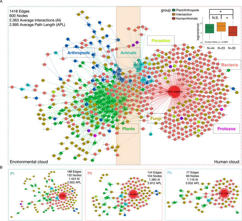
Fig. 7. — The bi-modal exposome interacting cloud. (A) The interaction network includes a plant-centric environmental cloud and a human-centric cloud. The intersection region between the two clouds is labeled by the dark yellow shade. The inset boxplots show that the species (detected in >= 50 samples) belonging to the Human/Animal group (human cloud) have significant less variance when compared to either Plant/Arthropods group (environmental cloud) or the Intersection group. Y-axis, log value of the variances of the aCPM values of analyzed individual species across all samples. (B) The individual exposome cloud of P1, P3, and P5 show diversity/complexity corresponding to their activity level. The number of average interactions (AI) is calculated at per node basis. The average path length (APL) is calculated by averaging the length of paths connecting any two nodes in the network. The Adj. p values are indicated as: N.S. Not Significant, * <0.05, ** < 0.01, *** < 0.001, and **** < 0.0001.

We hypothesized that human-related species would be less variable than environment-related species in our dataset because they are less susceptible to the macro temporal changes (Fig. 2E and F, Fig. 4E; Fig. S8B and C). To test this, we divided the implicated species (found in >= 50 samples) in the exposome network into three groups, namely Plant/Arthropods (representing the environmental cloud), Human/Animals (representing the human cloud), and the “Intersection” group with species that connect the two groups. We found that the Human/Animals group have significantly less variance than that of both Plant/Arthropods and the Intersection group (Fig. 7A inset). In contrast, we did not observe significant differences between the Plant/Arthropods and the Intersection” group. We also observed similar results when arthropods and animals were excluded from our analyses (Fig. S11I). We further demonstrated the reproducibility of the exposome network configuration using the data of P1, P2, P3 and found that each individual has a human-centric and an environmental-centric cloud; Fig. S11J-K).

To explore the utility of exposome networks at the individual level, we applied this technique to three different individuals in the case study (P1, P3, and P5, Fig. 3E-H) which had the same number of samplings. Based on these individuals, we observe that the complexity of personal exposome clouds are directly correlated with personal lifestyles and work-home routines. Specifically, the more active individual who travels to multiple locations, P1, has the highest number of nodes/edges/average interactions (AI) among the three, whereas P3 and P5 have decreasing complexity corresponding to their lifestyles (Fig. 7B), consistent with our earlier PCA analyses (Fig. 3E-H). Taken together, our exposome depicts a dynamic network of diverse species derived from at least two distinct ecosystems.

Discussion

Other metagenomics studies have investigated the microbiome in soil, extreme environments, and the ocean (Rinke et al., 2013; Sunagawa et al., 2015; Thompson et al., 2017). Although highly important for human health, airborne metagenomics are disproportionally understudied due to technological difficulties such as a) low density of microorganisms in the air, b) lack of an efficient method of retrieving information from such microorganisms, and c) bioinformatics challenges (Behzad et al., 2015). We have addressed these difficulties and produced a unique dataset that a) extends beyond the microbiome and also includes chemical exposures, b) is longitudinal and multi-location, and c) directly maps personal exposures. Our findings greatly extend the human microbial cloud to a human exposome cloud by including numerous organisms from different domains of life (Fig. 7A). Finally, the wearable device can easily be deployed as a portable miniaturized sampling station to monitor any geographical location.

In our chemical exposome, many of the potentially hazardous compounds were collected by sorbent adsorption from an air flow that already passed through a 0.8 μm pore-sized filter (for biological analyses). This indicates the possibility that the compounds could reach into the deep lower respiratory tract including respiratory bronchioles and alveoli and directly interact with the moist mucosa in lungs. However, neither the Environmental Protection Agency (EPA) nor the Center for Disease Control and prevention (CDC) has evaluated possible health risks associated with inhalation of these non-biological compounds, such as DEET. Our findings thus revealed a previously unrecognized type of potentially hazardous exposure that is commonly detected in the air.

Among the potential applications of our study, the putative location/lifestyle signatures are of high interest. Both biotic/abiotic exposures, as well as their correlations, show a strong location/lifestyle-driven pattern (Fig. 3 and 5), which can potentially define location-specific exposure profiles (“Campus” versus non-”Campus”). An archive with more individuals/locations could reveal more location-specific health-related substances, such as allergens, potential pathogens, and harmful chemicals, in human exposure. The understanding of location/lifestyle-specific exposures may benefit the population health at large, especially the immuno-compromised individuals.

Our study also provides invaluable data for ecological and evolutionary studies with the deeply sequenced metagenomics data. Most environment-related sequencing projects have targeted marker genes such as 16S/18S rDNA/rRNA (Barberán et al., 2015) and thus provide limited intraspecies diversity information, and no functional information. In comparison, our method is able to detect species across all domains of life, provide functional insights, and reveal intraspecies diversity at single-nucleotide resolution. The variation partitioning analyses revealed that different genera are subjected to drastically different influences from environmental and/or spatial/lifestyle sources (Fig. 3B), potentially relevant to their potential ecological niches. In addition, the capture and detection of rare taxa such as rotifer, various mites, and insects are impractical with targeted approaches (Fig. S4).

There are several notable limitations of our study: 1) We only followed 3 individuals extensively, hence some findings, such as the location-specific signatures, would benefit from the analysis of data from more individuals. Such information would help identify generalizable and individual-specific exposure dynamics. 2) Organismal sequence databases are still incomplete; hence misclassifications and false-negatives will occur. 3) For chemicals, the exact number and the nature of molecules is not known. Of the total of 2796 putative chemical features, only 972 can be tentatively annotated, most of which are potential toxins (Fig. S9). Future research using purified standards is necessary to confirm the numerous anonymous peaks.

Despite the limitations, the extent of diversity we observed in this study is enormous; In addition to over 2500 species identified, 5.11 million SNPs in 108 pan-domain species across all samples were identified. This number is comparable to the number of SNPs evaluated in the human gut microbiome (101 bacterial species; 3.98M SNPs at the individual level, 10.3 million for all samples) (Schloissnig et al., 2013). However, in spite of the great sequencing depth, the number of SNPs we found still severely underrepresents the true diversity in the human exposome (Fig. 6). In the biotic exposome, most contigs shared 70–90% identity to reference genomes, again suggesting our knowledge on intra- and inter-species diversity is limited (Fig. S3 and 4). 43.74% of DNA information cannot be classified even with our pan-domain and computationally intensive classification strategy (Fig. 1F). These results indicate that a huge gap exists between the complexity of our environmental exposures and what is presently in our knowledge database.

In the future, it will be important to systematically expand the depth and breadth of our exposure knowledge. These efforts will enable a comprehensive understanding of the diversity in our environmental exposures that eventually leads to an actionable exposure risk guidelines for general and personal human health.

STAR Methods

Contact for Reagent and Resource Sharing

Further information and requests for resources and reagents should be directed to and will be fulfilled by the Lead Contact, Dr. Michael Snyder (mpsnyder@stanford.edu).

Experimental Model and Subject Details

Personal environmental exposure sample collection

To measure personal environmental airborne exposures, 15 adult participants were recruited; all lived in the Northern California Greater Bay Area and some traveled to other locations, depending on the individuals. The participants enrolled in this study under the IRB protocols IRB-23602 and IRB-34907 at Stanford University. All participants are age 18 or older, self-reported healthy and consented in writing (See table below). All clinic measurements were covered by IRB-23602, with the enrollment criteria as age 18 or older. An RTI MicroPEM V3.2 personal exposure monitor (RTI international, Research Triangle Park, NC, USA) was modified and used to simultaneously collect biotic and abiotic samples of personal aerosol exposure for the period of August 2014 to January 2017. The MicroPEM allows for integrated sampling while simultaneously collecting real time particulate measurements (PM) using a 780 nm IR laser nephelometer operating on a 30-s cycling time. The original sequential oiled frit impactors were remove to maximize the biotic aerosol particulates collection. Before sampling and data collection, a 3.0 µm pore-size polytetrafluoroethylene (PTFE) 25 mm Teflon filter (PALL Corporation, Port Washington, NY, USA) or a 0.8 µm pore-size polyethersulfone (PES) 25 mm filter (Sterlitech, Kent, WA, USA) was placed in MicroPEM filter cassettes to collect aerosol particulates for biotics extraction. A homemade cartridge filled with 200 mg zeolite adsorbent beads (Sigma 2–0304) was also placed at the end of airflow to collect hydrophobic and hydrophilic chemical compounds. Before participants were given the MicroPEM monitor, the MicroPEM nephelometer was calibrated with an in-line HEPA filter, and pump flow rate was pre-calculated at 0.5 L per minute with a TSI model 4140 mass flowmeter (TSI, Shoreview, MN, USA) using Docking Station software (RTI international).

Participants were instructed to either carry the monitor on their arm or place the monitor near them within a 2-meter radius at all times during the sampling period. Once the participants turned the monitor on, sampling and monitoring would last for 1 to 14 days according to the participant’s activity. Three participants (P1, P2, P3) were sampled extensively; P1 for more than 2 years, P2 for approximately 1 year and P3 for three months intermittently. For P1, sampling was performed such that two filters were typically collected each week (one during the weekdays and one during the weekends). P1 traveled frequently and during each trip/location a dedicated MicroPEM monitor was used to collect the sample. If several locations were visited during one trip, a dedicated monitor and filter/cartridge would be used for each location separately and the filters were collect at the end of the trip. Samples from P2 and P3 were collected over longer intervals and samples often covered more than one location (1~2 weeks each time). At the end of the sampling and monitoring period, filters and cartridges were removed from monitor and stored at −80 ^oC until analysis. To minimize environmental contaminations, filters and cartridges were deployed and recovered from MicroPEM in a sterilized biosafety cabinet. The aerosol and quality control data were also downloaded from the MicroPEM monitor after each sampling through the Docking Station program. MicroPEM flow rate was post-calibrated after each sampling period using TSI 4140 mass flowmeter. All post-calibration flow rates were within ± 5% of pre-calibration values. Three participants (P1, P2, P3) also using MOVES App to track their geographic locations with GPS coordinates and daily activity.

Individual	Age	Gender/Sex
P1	61	Male
P2	45	Male
P3	61	Female
P4	40	Female
P5	36	Male
P6	60	Male
P7	31	Female
P8	43	Male
P9	36	Male
P10	31	Male
P11	28	Female
P12	29	Female
P13	43	Female
P14	56	Male
P15	42	Male

Open in a new tab

Method Details

DNA and RNA sample extraction and library preparation

After testing many extraction and amplification protocols we found the following protocol optimal for our studies. DNA and RNA were extracted from the filter using a modified protocol combining the PowerWater® DNA and RNA Extraction kits (Mo Bio, CA, USA) according to the manufacturer’s instructions. The amount of nucleic acid materials extracted from a typical sample filter is similar to that of 1–10 mammalian cell(s) (Fig. S1). The DNA and RNA extracts were then subjected to linear amplifications prior to library preparation for next-generation sequencing. Specifically, the DNA amplification was achieved through Multiple Displacement Amplification (MDA) with REPLI-g Single Cell Kit (Qiagen, Hilden, Germany). The RNA samples were linearly amplified by Ovation RNA-seq system V2 (NuGEN Technologies, Inc., San Carlos, CA, USA) following the manufacturer’s instructions. All pre-amplification steps were performed in a biosafety cabinet to minimize biotic aerosol particulate contamination from lab environment. Pre-amplification and post-amplification steps were carried out in physically separated locations. DNA and cDNA libraries were then prepared using the KAPA HyperPlus library kit (Kapa Biosystems, Wilmington, MA, USA) with Illumina® adaptors as described by the manufacturer. The size and quality of libraries were assessed on a Bioanalyzer instrument from Agilent (Agilent Technologies, Santa Clara, CA), and sequenced using Illumina HiSeq 4000 platform (2 × 151 bp) (Illumina Inc., San Diego, CA), with four samples pooled for each lane.

Through control experiments, we found that our approach produces reproducible results and is capable of detecting many species across domains of life (Fig. S2). Specifically, we carried out a control experiment where we employed two devices side by side at the same location to collect samples for 3 days and analyzed their filters through the pipeline in parallel. The taxonomy classification results for the two filters are highly concordant even at the species level (Fig. S2). Through comparisons with the other mainstream taxonomy classification pipelines, we found that our pipeline can classify significantly more contigs/reads across multiple domains, among which fungi, plants, and animals are not well covered by the default databases of other classification pipelines. Interestingly, due our unique pan-domain approach in species detection, we noticed that 18.3% and 20.7% of bases from DNA and RNA are classified as ambiguous even at the kingdom/subkingdom level, meaning they are similar to species belonging to different kingdoms. For example, a contig can be classified as an insect species as well as a bacterial or viral species. This either indicates contamination of reference sequences in existing databases or genuine host-cargo (pathogen) relationships.

Scanning Electron Microscopy (SEM)

The representative sample filters collected for SEM were dried using a vacuum desiccator (Bel-Art-SP Scienceware, Wayne, NJ, USA) overnight at room temperature. The dehydrated filters were then mounted onto a 12mm SEM stainless steel stub using double stick copper tape for maximum conductivity, followed by 50–100 Angstrom coating in an Au/Pd sputter coater for 2 minutes. The images were then visualized and taken by Hitachi S-3400N VP SEM (Hitachi High Technologies, Japan) and affiliated software.

Contamination considerations

Since our experimental protocol was adapted to low input nucleotide materials from environmental sources via unbiased linear amplification steps, we carefully evaluated the potential impact of contamination by including a blank filter for every batch of extraction-amplification-library preparations (28 batches). For each batch, we selected samples using the stratified random sampling method. Briefly, we divided our total samples into 15 groups each containing similar number of samples, which were collected during similar periods of time (e.g. #1–20, #20–40 etc.). We considered that the time of collection should play an important role in data variation and would likely represent the temporal variation in each batch. Unfortunately, we could not directly quantitate the absolute abundance of organisms following MDA amplifications. We evaluated the potential impact of contamination via the following approaches: 1. The quantitation of pre-amplified DNA and post-amplified cDNA (RNA could not be quantified without amplification) showed that there is at least a 8-fold difference in median concentration between blank/control filters and sample filters (Fig. S2A and B); this number is likely an overestimate of background since the single-cell amplification protocols were usually designed for samples with the very low amounts of material, giving the blank samples an opportunity to catch up; 2. The fact that the sequencing reads generated from the DNA blank/control filter is far less complex that those from the sample filters (Fig. S2C), based on the assembly results; 3. Through the UFC classification pipeline, the blank/control filters (Bacteria-heavy) show significantly different taxonomy profiles when compared to the sample filters (Fungi-heavy); 4. The fact that the batch effects play a very small role in our variation partition analysis (Fig. 3A and B) supports the notion that contamination is not a significant issue in our datasets; 5. Finally, population genetics analysis on blank/control filters and sample filters in parallel demonstrates orders of magnitude larger species intra-diversity on the samples filters relative to control filters (Fig. S2E-I; mapped reads were sub-sampled to the same coverage for sample and control filters). Further analysis indicates that while species identified in both blank/control and sample filters may share a portion of SNP sites (~60% of control SNPs), their actual allele profiles at such sites are drastically different (only share 3.7%). This result implies that for those species that can be detected in blank/control and sample filters, they are basically two distinct populations of the same species. Taken together, we believe the contamination plays an insignificant role in our dataset.

Chemical Compound Collection and Preparation

A homemade 3D-printed cartridge filled with 200 mg 13 angstrom (A) pore-size Molecular Sieve Adsorbent Sigma 20304 (Sigma-Aldrich Corp., St. Louis, MO USA) was attached to the end of the particle-free air flow in the portable device to collect abiotic chemical air solvent concomitantly with the collection of biotic biological particulates in personal environment exposure.

The adsorbent zeolite beads were later recovered in a clean Eppendorf LoBind tube, where 1 ml methanol (Mass Spec grade) was added. The mixture was incubated for 20 min at room temperature (RT). Then separated at 22,000 x g for 20 min at RT. The supernatant was transferred to 150-µl deactivated glass insert housed in Waters 2-ml brown MS vials for LC/MS analysis, or stored at 20 °C for later use.

For chemical compounds, we used zeolite adsorbent to collect air-dissolved compounds from particle-free air flow that was concomitantly generated with the collection of biotic samples. Zeolite is widely used as molecular sieve to remove molecular impurity in industry. Among our different sample testing, zeolite was able to readily capture two flavor compounds emanated by an orange peel placed in close vicinity (Fig. S3D and E).

Liquid Chromatography Coupled Mass Spectrometry (LC/MS)

LC/MS analysis was performed in a platform that consists of Waters UPLC-coupled Exactive Orbitrap Mass Spectrometer (Thermo, Waltham, MA, USA), using a mix-mode OPD2 HP-4B column (4.6×50 mm) with a 4.6×10 mm guard column (Shodex, Showa Denko, Tokyo, Japan). The column temperature was maintained at 45 °C. The sample chamber was maintained at 4 °C.

The binary mobile phase solvents were: A, 10 mM Ammonium acetate (NH4OAc) in 50:50 Acetonitrile:water; B, 10 mM NH4OAc in 90:10 Acetonitrile:water. Both solvents were modified with 10 mM Acetic acid (HOAc) (pH 4.75) for positive mode acquisition, or 10 mM NH4OH (pH 7.25) for negative mode.

The flow was set as follows: flow rate, 0.1 ml/min; gradient, 0–15 min, 99% A, 15–18 min, 99% to 1% A; 18–24 min, 1% A; 24–25 min, 1% to 99% A; 25–30 min, 99% A.

The MS acquisition was in profile mode and performed with an ESI probe, operating with capillary temperature at 275 °C, sheath gas at 40 units, spray voltage at 3.5 kV for positive mode and 3.1 kV for negative mode, Capillary voltage at 30 V, tube lens voltage at 120 V and Skimmer voltage at 20 V. The mass scanning used 100,000 mass resolution, high dynamic range for AGC Target, 500 ms as Maximum Inject Time and 70–1,000 m/z as the scan range.

Quantification and Statistical Analysis

General statistical analysis and data visualization

The majority of statistical analyses and visualizations were done in Rstudio and R (at the time of writing, 1.0143 for Rstudio and 3.4.0 for R), with necessary aid from customized python scripts (2.7.4) and shell scripts (Linux). The primary R packages are mostly maintained by the Bioconductor project (https://www.bioconductor.org/, along with all their dependencies). The essential ones used are ggplot2 (2.2.1), reshape2 (1.4.3), edgeR (3.18.1), NMF (0.23.6), phyloseq (McMurdie and Holmes, 2013) (1.20.0), RColorBrewer (1.1–2), scales (0.5.0), corrplot (0.84), Hmisc (4.1–1), ggrepel (0.7.0), vegan (2.4–5), cluster (2.0.6), factoextra (1.0.5), plyr (1.8.4), dplyr (0.7.4), psych (1.7.8), glmnet (Friedman et al., 2010) (2.0–13), devtools (1.13.4), ggpubr (0.1.6), tidyverse (1.2.1), ade4 (1.7–10), caret (6.0–78), e1071 (1.6–8), pROC (1.10.0), gridExtra (2.3), ggnetwork (0.5.1), ggsci (2.8), ggbeeswarm (0.6.0), ggpmisc (0.2.16), ggmap (2.7), colorspace (1.3–2), adespatial (0.1–1), limma (3.32.10), and relaimpo (2.2–2), PMA (1.0.9). The main analysis script is attached as Data File 1.

In general, non-parametric statistical tests (Wilcoxon test, Kruskal-Wallis, and Spearman correlation) were used over the parametric counterparts due to the non-normality of our datasets. We adjust the p values using the Benjamini & Hochberg (BH) method to control for False Discovery Rate (FDR), when multiple comparisons are concerned, including p value matrix constructed when calculating correlations matrix among different features or samples. We chose not to rarify our data because we do not want to lose any data (McMurdie and Holmes, 2014). For inter-sample normalization, we chose to not use the standard negative binomial or rlog modeling approaches (implemented in edgeR and DEseq2 (Love et al., 2014)) because our exposome data violates the fundamental assumption that most features should not change drastically in-between samples. Instead, we used Counts Per Million (CPM) method (Love et al., 2014) for inter-sample normalization followed by hyperbolic arcsine (arcsinh) transformation (asinh() in R) for within sample normalization (Callahan et al., 2016). We used log₁₀(n + 1) transformation for chemical abundances. The arcsinh transformed CPM values (aCPM) were used in all statistical/computational analyses and visualizations unless otherwise noted (e.g. area plots of relative abundances of kingdom/subkingdom in Fig. 2A-D and pathogen analysis). We did not adjust relative abundance value based on genome sizes of different organisms because a lot of species in our database are represented by incomplete genomes (a collection of contigs), therefore precise estimates of their genome sizes cannot be achieved. We used the F1000 microbiome workflow paper as a reference in designing many of the downstream analyses (Callahan et al., 2016). Annotated phylogenetic trees were generated using phyloT and iTOL (Letunic and Bork, 2011).

Moran’s Eigenvector Map (MEM) is a statistical method to extract spatial structure information from geographic coordinates of samples collected from different locations, typically used in the ecological studies. Statistically, Moran’s Eigenvector Map (MEM) variables are orthogonal vectors maximizing the spatial autocorrelation (Dray et al., 2012) (measured by Moran’s I of autocorrelation). MEM variables are calculated from the spatial neighborhood matrix and spatial weighting matrix, both of which are derived from the raw spatial data of the sampling sites. Each MEM variable independently represents broad- or fine-scale spatial structure in the geographic data, and can be directly super-imposed on the geographic coordinates for visual interpretation of spatial patterns (Fig. S6A). In this study, we used adespatial, ade4, and spdep packages to construct the MEM variables using the geographic coordinates of collected exposome samples. The MEM variables were forward-selected on the taxonomy abundance data using redundancy analysis (RDA) to filter insignificant MEM variables. We then used the selected MEMs to provide explicit spatial information in the downstream variation partitioning analysis.

For differential abundant genera/phyla/species analyses between the “Campus” and non-”Campus” locations and across four seasons, we only considered organisms (at different taxonomy level) that were detected in more than 50 of 283 samples. We used the Wilcox test for two group comparisons and the Kruskal-Wallis test for multi-group comparisons. For ad-hoc comparisons we used the Wilcox test. P values for multiple comparisons (including ad-hoc comparisons) were adjusted using the BH method. Comparisons with Adj. p < 0.05 were reported accordingly.

For ordination methods, we chose principal component analysis (PCA) instead of the correspondence analysis (CA) because we were able to observe a environmental gradient axis shorter than 2 in the detrended correspondence analysis (DCA) (Fig. S6C). This indicates that the environmental gradients in our dataset are rather short and linear instead of unimodal for which CA is designed (Smilauer and Lepš, 2014). All ellipses are drawn with axes equal to the standard deviation of the data unless noted otherwise. For variable plots, contributions of individual variables are calculated from the weighted average of the square of their coefficients (loading score) for top three principal components (weighted by principal components’ eigenvalues). As a validation of our PCA analysis results, we also calculated pairwise in-group and out-of-group Bray-Curtis distances of respective groups and show that the differences are statistically significant.

For overall variation partitioning, we used dbRDA (distance based redundancy analysis) to decompose the variation in our datasets influenced by various variables, we gathered and prepared 64 metadata variables for each sample; we divided them into “environmental”, “spatial/lifestyle”, and “technical” groups and carried out forward-selection of variables within each group (this is to retain the overlapping between different groups). We then partitioned the variation (squared Bray-Curtis distances) of our dataset based on the definitions of these groups of variables using the varpart() function from the vegan package. Adonis (improved PERMANOVA) analysis was used to evaluate how variation can be explained by individual variable.

For genus-based variation partitioning, we selected genera that were detected in more than 100 samples, 241 genera satisfied this criterion. We then performed forward-selection on all 64 variables over the entire exposome DNA dataset to select the best representative variables. Multivariate linear regression models were then constructed for each of the 241 genera and based on the adjusted p value (p < 0.05, BH) of these models, we selected 199 genera for the downstream variation decomposition analyses. To evaluate the contributions of each variable, we used a hierarchical partitioning method implemented in the relaimpo package, which loops through all potential ways of adding the terms in regression models (instead of evaluating the R² based on one particular regression model). After the contribution of each variable was evaluated in conjunction with all other variables, we calculated the contributions of each group (environmental, spatial/lifestyle, and technical) by summing up the contributions of the variables of each group. Note that the total percentage of contributions of each group is based on the total explained variation of each individual model, not the total variation.

The formula used for the multivariate regression model constructed for individual genus (see Fig. S6 for an explanation on these variables):

a s i n h (C P M) \sim b a t c h + l o n g i t u d e + M e a n_T e m p e r a t u r e C + m F P A R + M E M 1 + s p r i n g + O v e r a l l . A Q I . V a l u e + M E M 91 + w i n t e r + P 1 + d a t e . m o n t h + p o p d e n s i t y + M E M 69 + d N 02 + P 2 + M E M 83 + i s_t h e r e_r a i n

For sparse canonical correlation analysis (sCCA), we first evaluated the correlations between the biological (biotics) and chemical (abiotics) dataset and show that these two datasets have extensive correlations among their features (p < 0.05, 499 permutations, implemented as the RV.rtest() function from the ade4 package, Monte-Carlo Test on the sum of eigenvalues of a co-inertia analysis). We then performed sparse canonical correlation analysis using the penalized matrix decomposition (implemented as the CCA() function from the PMA package) on the two datasets with penaltyx = 0.20, penaltyz = 0.20. We combined biological/chemical features with non-zero coefficients and performed PCA analysis on the combined data frame to visualize the driving force behind the correlations (Callahan et al., 2016).

UFC classification pipeline

Raw reads in fastq format were first removed of duplicates using an in-house developed python script. We removed only exact paired-end duplicates (meaning both forward and reverse reads need to be identical, although the ordering of which can be swapped). We expected most of pair-ended duplicates represent technical artifacts as we applied linear amplification step to both DNA and RNA during sequencing library preparations. The de-duplicated reads were then trimmed using Trim_galore (0.4.4) wrapper with default parameters (https://github.com/FelixKrueger/TrimGalore), which essentially combines the adapter removal tool Cutadapt (1.14) and NGS quality control tool Fastqc (0.11.5). These reads were then mapped to hg19 human genome using BWA-mem algorithm with default parameters. After removing human-mapped reads, a de novo assembly step was executed by Megahit (Li et al., 2015) (1.1.1), a popular de bruijn graph assembler for short NGS sequencing reads. This step assembled millions or more reads into a much smaller collection of information-dense contigs (>200 bp).

These contigs were queried against the UFC database using a BLASTN (2.3.0+) wrapper, which takes NCBI BLAST algorithm as its core and added a few modified functionalities that are essential to the pipeline. The choice of database(s) is the most crucial component when it comes to nucleic acids detection and classification. A poorly chosen database always leads to under-classification and sometimes even miss-classification. For the accurate identification of organisms, a broad database encompassing all domains of life is essential. In short, our in-house UFC database is constructed by a union of NCBI Refseq project and the Genbank representative genomes, containing nucleic acid information that represents all domains of life. This curated database includes all domains of life known to humans, which are broadly divided into the following categories: plants, protozoa, invertebrates, bacteria, archaea, fungi, virus, non-mammal vertebrates and some selected animals (82 million entries, 40,000 species).

The BLAST results were further analyzed by a customized implementation of Lowest Common Ancestor (LCA) algorithm, along with special considerations to certain domains of life that do not conform to the usual taxonomy database structures. The UFC taxonomy database was constructed by leveraging the NCBI taxonomy database to provide a unique taxonomy label for each entry in the UFC database, which enables fast and accurate evaluation of taxonomy in the LCA step. The inferred taxonomy results from the LCA step was compiled and displayed in a text format. Specifically, the report followed the hierarchical taxonomy rank conventions of NCBI and displayed the sequencing abundance of each taxonomy rank in aggregate. We would like to emphasize that although classification down to the species level is possible, the conservative LCA algorithm will rigorously classify contigs at higher taxonomy level due to ambiguity in the sequence alignments. Abundance estimation was handled as aggregated sequencing amount (applicable to all taxonomic levels). The sequencing amount (in base pairs) was estimated by mapping sequencing reads that were used for assembly onto the assembled contigs, each with assigned taxonomy label. The final report also included a special section where species belonging to different groups of interests were listed separately.

Although our pipeline classifies contigs at the species level, we noticed that frequently those contigs would share 70%−90% identity with target reference genome (Fig S4). This indicates that while a taxonomic label is assigned, the contig is actually only classified by its most closely related species in the database. Although our UFC database is substantially larger than most, if not all, known fragment classification pipelines, the actual diversity in nature still dwarfs our current knowledge database of species. This observation is also reflected in the results of population genetics analysis where substantial intraspecies diversity was observed for almost all involved species across different domains (Fig. 6). Effectively, environmental species should be viewed as a dynamic species complex defined by the aggregate functional capacity and intraspecies diversity of each member of the complex. As examples, the information on contigs classified as Rotifera and Apicomplexa organisms is attached in Data File 2.

Coassembly of DNA and RNA data

To gain an overview understanding of our data, we co-assembled 42.9 and 30.4 billion reads for DNA and RNA exposomes, respectively (totaling 6.43 and 4.56 Tbp). Due to the sheer amount of data, even megahit that was optimized for assembling large amount of metagenome data could not handle the job given the limitations on computing resources. To overcome this, we used a digital normalization module implemented in bbnorm (37.02), a part of the bbtool package (https://jgi.doe.gov/data-and-tools/bbtools/), to significantly reduce the amount of input reads. We then used megahit (Li et al., 2015) (1.1.1) with the preset --sensitive option for the co-assembly. For DNA, the co-assembly comprised of 6,545,607 contigs, totaling 7,409,478,621 bp, with cutoff set at 200 bp, a max contig size of 111,652 bp, an average contig size of 1132 bp, and a N50 of 1896 bp. For RNA, the co-assembly comprised of 1,023,712 contigs, totaling 492,353,963 bp, with cutoff set at 200 bp, a max contig size of 169,362 bp, an average contig size of 481 bp, and a N50 of 486 bp. We ran the co-assembled contigs through our UFC pipeline and the classification results are consistent with the aggregate results from analyzing individual samples incrementally (The N+1 problem).

Bootstrap confidence interval estimation, bootstrap-based dominating force definition, and the permutation-based p-value estimations

We used the bootstrap method to evaluate the 90% confidence interval of selected calculated or measured statistics based on the genus abundance data (denoted as S), such as relative importance of each group of variables (Environmental, Spatial/lifestyle, and Technical artefacts), denoted as $k_{1}, k_{2}, \dots k_{n}$ , collectively defined as the statistics vector K. We resampled the genus abundance data with replacement 9999 times (also known as bootstrapping). For each of the resampled abundance data ${S^{'}}_{1}, {S^{'}}_{2}, \dots {S^{'}}_{9999}$ , we retain all corresponding meta-variable associations, and calculated the relative importance and other statistics vectors ${K^{'}}_{1}, {K^{'}}_{2}, \dots {K^{'}}_{9999}$ for the each S’. We then computed the difference between the K and each of the ${K^{'}}_{1}, {K^{'}}_{2}, \dots {K^{'}}_{9999}$ vectors, resulting in a 9999 ∗ n matrix of differences denoted as D. For each column of the matrix D, we sorted the values from lowest to the highest and calculated the values for 5th percentile and 95th percentile of each column, denoted as P₅ and P₉₅, respectively. The 90% confidence interval for each of the statistics $k_{1}, k_{2}, \dots K_{n}$ can then be estimated as $[k_{n} - P_{95}, k_{n} - P_{5}]$ , where k_n is the value of the statistic evaluated using the original dataset.

For each genus, we consider it is subjected to the dominating influence from either the environmental variables (Env) or spatial/lifestyle (Spa) variables, if the calculated relative importance of one group is consistently greater than the other in at least 90% of all 9999 bootstrap samples, namely ${S^{'}}_{1}, {S^{'}}_{2}, \dots {S^{'}}_{9999}$ For example, for genus A, if the calculated relative importance of the environmental variables env is greater than the calculated relative importance of the spatial/lifestyle variables spa in 93% of the bootstrap samples, we define that the genus A is subjected to the dominating force from the environmental variables env in our dataset.

For permutation test, we permutated the meta-data associations with the taxonomy abundance profiles randomly 9999 times and recalculated the relative importance of each group of variables (as well as other statistics) for each genus in the 9999 permutated datasets. We then derived the p-values by calculating 1 – q, where q is the quantile value of the observed value of the statistics in the background distribution of the permutated statistics, as evaluated by the 9999 permutated datasets.

Analysis of the source of dominating influence in bacteria, plants, and animals.

Using the same criteria in the fungi variation partitioning analysis, 5 bacterial genera, 4 of them being Firmicutes, are subjected to dominating environmental forces (blue), including Bacillus, Flavobacterium, Enterococcus, and Dolosigranulum (Fig. 3B, second panel). 6 bacterial genera are subjected to dominating spatial/lifestyle influence (dark yellow, some are overlapping), including Corynebacterium (skin bacteria), Acinetobacter (soil bacteria, but also found in hospital infections), Dyadobacter, and Geobacillus (Fig. 3B, second panel). The plant genera with dominating environmental influences (blue) are Quercus (oak tree), Fraxinus (ash tree), and Musa (banana tree). In contrast, Betula (small tree/shrubs), Triticum (wheat/grass), and Aegilops (grass) have dominating influences from Spatial/lifestyle variables (dark yellow). Thus, it appears that, based on our data, larger plants such as trees (Diamonds in Fig. 3B, third panel) are more likely to be influenced by environmental variables (such as seasons, see below) whereas the exposures to smaller plants such as grass (Circles in Fig. 3B, third panel) may be more Spatial/lifestyle-dependent. Finally, animal genera Canis (dogs) and Felis (cats) are both strongly spatial/lifestyle-dependent (>60%), reflecting their presence at distinct geographical locations (Fig. 3B, last panel). We also noted that the abundance of a fly genus, Rhagoletis, is subjected to substantial technical influence.

Graph-based permutation test

To demonstrate the seasonal influence on the exposome, we first calculated the Bray-Curtis distances between all DNA exposome samples at the genus level. We then constructed nearest neighbor (NN) tree with the number of neighbor set as 1 (knn = 1). We colored each node in the resulting tree based on the sampling seasons. If two nodes (samples) are of the same season, the edge connecting them is “pure”. Otherwise, the edge connecting them is “mixed”. We then counted how many pure edges there are in the initial tree. To test whether this number is statistically significant above background distribution, we permutated the season labels of all nodes while maintaining the initial tree structure (Callahan et al., 2016). For each permutation, we count the number of pure edges and mixed edges. As a result, we generated a background distribution of the number of pure edges (and mixed edges) for the original tree (N = 9999 in this study). We then calculated the chance of observing the number of observed pure edges (or greater) in the original tree based on this background distribution. Due to the limitation of permutation-based p value estimation method, we cannot derive a p-value less than 1/N (or p = 0.0001) in this study, hence the actual probability may be lower.

Fuzzy c-means clustering

We used the fuzzy c-means clustering algorithm (package e1071) to explore the seasonal and location-related patterns in our biotic and abiotic data, respectively. For seasonal clustering, we binned the DNA relative abundance (aCPM) data by seasons for all samples (arcsinh transformed CPM at the genus level). This produced a N ∗ 4 data matrix where N is the number of genera in the dataset. For chemical data, we directly used the log transformed, log(n + 1), chemical abundance data over 15 locations (N ∗ 15). We used default parameters (except for iter.max = 2000). The optimal cluster number was determined based on a combination of three methods (Elbow, Silhouette, and Gap statistic). The clustering results were then optimized by visualizations of the results (PCA and line plots). For line plots, only features (both biotics and abiotics) with a membership score > 0.65 were considered, we chose this high stringency so that we can explore the dynamics of the core members of each cluster. In fuzzy c-means clustering, the membership score is the probability of a feature belonging to any cluster, each feature is assigned a cluster based on its top membership score (as opposed to k-means clustering, where the membership score is binary). The alpha (transparency) of each feature is directly based on the membership score. The output results were not smoothed.

Season predictive modeling

To predict seasons based on the DNA taxonomic profile across different domains of life, we developed a customized R script pipeline using the glmnet package. Specifically, we used the LASSO logistic regression classifier implemented in the glmnet package, because it generates a classifier with a small number of selected features from the thousands of genera in our data. These features are biologically interpretable as the linear combinations of variables in the logistic regression. Since the feature selection process is built into the LASSO classifier, it is straightforward to obtain not only the prediction model, but also a realistic estimate of the generalized error during cross-validations. This is superior to a two-step approach, where a supervised feature selection step is performed prior to cross-validation, which can lead to over-optimistic accuracy estimates. In addition, this approach prevents information leakage from highly correlated features between training and testing dataset. As only one of the highly correlating features will be selected before model training/testing.

Specifically, the steps are:

Applying arcsinh transformation to our dataset, which performs nearly linearly for small values, but near log transformation for larger values.
Selecting the data of P1 in North America (N=179) because the variabilities in other continents with limited sample sizes did not allow adequate in depth analysis. We use the genus level datasets because they provide the best balance between resolution and accuracy.
Partitioning data for ten-fold (outer loop) times ten folds (inner loop) nested cross-validations. In the outer loop, one fold of data is progressively assigned as the testing data, the remaining nine folds of data are then progressively partitioned into one plus nine folds in the inner loop. The nine folds of data are used for training the model to get a hyperparameter for selected model (in this case, the penalizing parameter lambda for feature selection) and the one fold of data is used for evaluating the hyperparameter for selected model (in this case, the penalizing parameter lambda for feature selection). The resulting model from the internal loop is then tested on the one fold in the external loop, this step generates a series of model performances parameters including multi-class area under curve (mAUC), accuracy, specificity, F1 score etc. We resample the whole dataset 10 times to generate 100 internal model performance parameters to assess its stability. Weights for samples in each season are adjusted for every training to account for sample size variations in four seasons.
We obtained season prediction scores for each sample based on the average prediction scores of the resampled 10×10 internal testing, from which we generated the multi-class ROC curve using one vs all approach for each season, using mean predicting scores of each season.
For model interpretation and feature extraction, we examined features with non-zero coefficients for each season and visualized them on a heatmap. For importance of features, we use square of coefficient normalized by total sum of squared coefficient for each season to denote its contribution to the prediction model. Bar length of lollipop plot corresponds to the log-odds ratios of respective feature.
For external validation, we used the data from P2, who stayed in the North America region throughout the entire sampling period, making it a great external validation dataset. The result is comparable to the performance metrics through cross-validation on P1’s data.

Of note, this algorithm does not retain certain genera due to multicollinearity issues (if several genera are highly correlated, only one of them will be selected for model training purposes), which are fairly ubiquitous due to seasonal patterns of many genera as previously discussed. However, as we demonstrated in the results, the selected features indeed reflect the seasonal patterns consistent with the season predicting model.

Season predictive model identified species with corresponding seasonal patterns.

Examples include: a) the winter-contributing genus Tricholoma, a type of edible mushroom that grows in winter; b) the spring-contributing genus Azadirachta, a type of tree that blooms during the spring; c) the summer-contributing genus Sclerotinia, or white mold, which sheds spores during summer (Fig. 4J). Interestingly, the aquatic Flavobacterium was identified as a winter-contributing genus (Luria et al., 2016) (Fig. S8G, right), indicating that we captured organisms that are not previously considered as airborne.

Population genetics analysis

For population genetics analysis, we adapted the method from previous human microbiome studies (Kuleshov et al., 2016; Schloissnig et al., 2013). Specifically, we first generated a list of reference genomes with > 10x aggregate coverage among all samples. We chose the reference genomes based on clinical and scientific interests for each domain. For bacteria, the focus was placed on pathogens, opportunistic pathogens, and human related species, in that order. For fungi, the focus was placed on mold species. For viruses, we chose the top 21 species as all of their coverage are quite high among samples. For species with draft genomes comprised of assembled contigs instead of complete chromosomes, we only considered contigs longer than 1000 bp in our analysis. Reference genomes/contigs with less than 10% coverage were discarded from the final analysis. An assembly of reference genomes and contigs was used as the reference to map total pooled DNA reads (for RNA viruses, total RNA reads were used). We followed the BROAD Institute variant calling best practices until the actual variant calling step, for which we developed a custom SNP calling pipeline based on previous studies (Kuleshov et al., 2016; Schloissnig et al., 2013) and only considered bases with a quality score >= 15. We required SNPs to be supported by >= 4 reads and to occur with a frequency of at least 1%. This rules out sequencing errors. We opted to use custom variant caller because the variant calling in our dataset require special considerations in the number of haplotypes existed for a particular species which is an unknown number, therefore all optimizations in the existing variant calling procedures for human genome are not applicable. We also detected indel variations but the results was not used in population genetics analysis.

We estimated SNP density (Number of SNPs/kbps) and nucleotide diversity (π) based on the SNP profiles. The nucleotide diversity (π) for each SNP site is calculated using the following formula:

π = \sum_{i j} x_{i} x_{j} π_{i j} = 2 * \sum_{i = 2}^{n} \sum_{j = 1}^{i = 1} x_{i} x_{j} π_{i j}

where x_i and x_j are the respective frequencies of the i th and j th sequences (each “sequence” is only one base here) at each site, π_ij is the number of nucleotide differences between the i tℎ and j tℎ sequences (either 0 or 1), and n is the number of coverage at each site. The calculated nucleotide diversity of each site is then aggregated over entire reference genome or contigs to calculate the nucleotide diversity of the respective species. For species with unfinished genomes (collection of contigs), we calculated weighted versions of the metrics using their effective genome sizes (proportion of genome that have >= 4x coverage) as weights. To validate, our results are consistent with population-level estimation published previously for bacteria (Kuleshov et al., 2016; Schloissnig et al., 2013). In addition, our results show that even multiple chromosomes from the same viral species have similar SNP density and nucleotide diversity even if the coverages are different (Fig. S11).

Transcriptomics analysis

Contigs from the co-assembled RNA were mapped using BlastX to the non-redundant (nr) protein database from NCBI. RPS-BLAST was used to annotate protein functions based on Conserved Domain Database. Gene products were annotated using gene ontology (GO), cluster of orthologous groups (COG), protein family (Pfam) and protein clan databases. Enrichment was calculated relative to the observed GO annotations across all taxonomic groups in the transcriptomic dataset. Results were visualized using R.

Allergen characterization

Taxonomy categorization of the co-assembled RNA contigs was performed using the in-house UFC pipeline. This information, along with Pfam annotations, were further used to identify potential allergens using the structural database of allergenic proteins (SDAP). We were able to identify 42 potential allergen proteins, 31 of which are non-food related. To calculate allergen abundance, we mapped the RNA sequencing reads from each filter to the identified allergen contigs. Sequence mapping was performed using Burrows-Wheeler Aligner (BWA). Gene expression levels were calculated in CPM.

Species interaction network (Exposome clouds)

To generate the species interaction network, we first acquired a list of species of interests from either all samples or samples of individuals in case studies. We integrated two species interaction databases to generate a comprehensive species-interaction database that cover pathogen-host and other natural interactions between species of different domains (Poelen et al., 2014; Wardeh et al., 2015). We then queried our species list against the species-interaction database. Only interactions with both species found in our query list are retained. The results were parsed using customized scripts to comply to the import format of Gephi (0.9.2). The layout algorithm (Yifan Hu) was chosen with customized parameters to optimize the visualization of the exposome clouds of interest in Gephi.

Chemicals post-acquisition analysis

The raw LC/MS data files were centroided with PAVA (Guan et al., 2011) and converted to mzXML format by a customized R script. Mass feature extraction was performed with XCMS v1.30.3. The mass features were then manually searched against the Metlin metabolite database using 5 p.p.m. mass accuracy, with Toxicant search turned on. A portion of the metabolite hits were validated using standards that were analyzed in an identical fashion (e.g Fig. S9). The scored mass features were clustered with SIMCA v14.1(Umetric, Malmö, Sweden). For a conservative assessment of the number of unique chemical features, we developed a customized Python script to remove potential isoforms, isotopes, and adducts from the 3,299 xcms-extracted putative chemical features that were enriched at least 10 fold as compared with the blank control. Filter windows of m/z differences (±0.0015, corresponding to 6 p.p.m at 500 m/z or 10 p.p.m at 300 m/z) and retention time (±0.1 min) were applied. We estimated the total number of at least 2,796 unique chemical features that cannot be considered as isoforms (e.g. the same mass within the same retention time window), isotopic mass species (¹³C for M+1, ³⁴S or ¹⁸O for M+2), or adducts (-H₂O, +Na, +NH₄, +Cl) of another feature in the data. We note however that all adducts and modifications of compounds are not known so this estimation is tentative. The predicted accurate masses for isotopic peaks and adducts were obtained from XCalibur (V2.2 Thermo), the same software used to acquire all mass spectrometry data in this study.

Identification of genera that influence sample clustering patterns in the four-people tracking study

We investigated which genera influenced the clustering patterns (Fig. 3H). P6’s device captured signatures of Alkanindiges, Metaseiulus, Propionibacterium, and Mogibacterium genera (Fig. 3H navy boxes). Alkanindiges is a genus of bacteria typically found in an urban environment, usually in sludge; Metaseiulus is a type of mite frequently found indoors; Propionibacterium, a genus of bacteria, is usually found on human skin; Mogibacterium is an obligate anaerobic bacterial genus that is associated with human periodontitis. These genera are expected in urban/indoor/human environment, consistent with P6’s location. In contrast, P1’s more active schedule led to significant amounts of plant and fungi exposures (Fig. 3H green boxes). Overall, these results demonstrate an important role of spatial/lifestyle-related variables in our exposome dynamics.

Data and Software Availability

The raw sequencing reads for DNA and RNA, as well as the co-assembled contigs from the DNA and RNA reads, are deposited under the NCBI Bioproject PRJNA421162. The main analysis script was written in the Rmarkdown format and is attached as Data File 1. The detailed information for contigs assigned as Rotifer and Apicomplexa is included in the Data File 2. Please see the Key Resources Table for availability of other software.

KEY RESOURCES TABLE

REAGENT or RESOURCE	SOURCE	IDENTIFIER
Antibodies
Bacterial and Virus Strains
Cowpea mosaic virus	Dr. Dinesh Kumar, UC Davis	N/A
Biological Samples
NATtrol Respiratory Validation Panel (RVP) (Qualitative)	ZeptoMetrix Corporation	NATRVP-3
Chemicals, Peptides, and Recombinant Proteins
Pyridine	FISHER SCIENTIFIC	AC131780500
Octanoic acid	Sigma	C2875–10ML
Hexanoic acid	Sigma	53745–2.5G
Decanoic acid	Sigma	C1875–100G
N,N-diethyl-m-toluamide (DEET)	Fisher Scientific	AC114571000
Tangeretin	Fisher Scientific	505943
Nobiletin (Hexamethoxyflavone)	Fisher Scientific	505360
Phthalate	Sigma	90677–100ML
Diethylene glycol	Sigma	03128–5ML-F
Omethoate	Sigma	36181–100MG
Critical Commercial Assays
The Ovation RNA-Seq System V2	NuGEN	7102–32
PowerWater® DNA kit	Qiagen-Mo Bio	14900–100-NF
PowerWater® RNA kit	Qiagen-Mo Bio	14700–100-NF
REPLI-g Single Cell Kit	Qiagen	150343; 150345
HyperPlus library kit	Roche-Kapa Biosystems	KK8514
Deposited Data
Raw sequencing reads for DNA and RNA	This study	NCBI Bioproject PRJNA421162
Co-assembled contigs for DNA and RNA	This study	NCBI Bioproject PRJNA421162
Experimental Models: Cell Lines
Experimental Models: Organisms/Strains
Oligonucleotides
Recombinant DNA
Software and Algorithms
Moves App	ProtoGeo Oy	N/A
R analysis script	This study	Data File 1
PAVA	PMID: 21937731	https://www.ncbi.nlm.nih.gov/pubmed/21937731
Rstudio	https://www.rstudio.com	https://www.rstudio.com
Bioconductor package	https://www.bioconductor.org/	https://www.bioconductor.org/
DESeq2	PMID: 25516281	https://genomebiology.biomedcentral.com/articles/10.1186/s13059–014-0550–8
phyloseq	PMID: 23630581	https://www.ncbi.nlm.nih.gov/pubmed/23630581
reshape2	https://www.rdocumentation.org/packages/reshape2/versions/1.4.3	https://www.rdocumentation.org/packages/reshape2/versions/1.4.3
ggplot2	https://github.com/hadley/ggplot2-book	https://github.com/hadley/ggplot2-book
edgeR	PMID: 19910308	https://www.ncbi.nlm.nih.gov/pubmed/19910308
NMF	PMID: 20598126	https://www.ncbi.nlm.nih.gov/pubmed/20598126
RcolorBrewer	https://cran.r-project.org/web/packages/RColorBrewer/index.html	https://cran.r-project.org/web/packages/RColorBrewer/index.html
vegan	https://cran.r-project.org/web/packages/vegan/index.html	https://cran.r-project.org/web/packages/vegan/index.html
factoextra	https://cran.r-project.org/web/packages/factoextra/index.html	https://cran.r-project.org/web/packages/factoextra/index.html
glmnet	PMID: 20808728	https://www.ncbi.nlm.nih.gov/pubmed/20808728
e1071	https://cran.r-project.org/web/packages/e1071/index.html	https://cran.r-project.org/web/packages/e1071/index.html
relaimpo	https://cran.r-project.org/web/packages/relaimpo/index.html	https://cran.r-project.org/web/packages/relaimpo/index.html
ade4	https://www.jstatsoft.org/article/view/v022i04	https://www.jstatsoft.org/article/view/v022i04
ViromeScan	PMID: 29492895	https://www.ncbi.nlm.nih.gov/m/pubmed/29492895/
PubChem	PMID: 15879180	https://pubchem.ncbi.nlm.nih.gov
phyloT	PMID: 27095192	https://phylot.biobyte.de
iTOL	PMID: 27095192	https://itol.embl.de
megahit	PMID: 25609793	https://github.com/voutcn/megahit
bbtools	https://jgi.doe.gov/data-and-tools/bbtools/	https://jgi.doe.gov/data-and-tools/bbtools/
Bwa-mem	https://arxiv.org/abs/1303.3997	http://bio-bwa.sourceforge.net
Gephi	https://www.aaai.org/ocs/index.php/ICWSM/09/paper/view/154	https://gephi.org
XCalibur	Thermo-Fisher Scientific	https://www.thermofisher.com/order/catalog/product/OPTON-30487
SIMCA	Umetric	https://umetrics.com/products/simca
Other
ODP2 HP-4B (LC column)	Shodex	F009121
OPD2 HPG-4A (LC guard column)	Shodex	G207063
Information and statistics on classified contigs of Rotifer and Apicomplexa	This Study	Data File 2
MicroPEM Personal Aerosol Exposure Monitor v3.2A	RTI International	N/A
Teflo Air Sampling Filters	PALL Life Science	R2P1025
Polyethersulfone Membrane Filters	STERLITECH Corporation	PES0825100
The TSI Mass Flowmeter	TSI Inc	Model 4143 D
Bioanalyzer	Agilent	G2939BA
Illumina HiSeq 4000 platform	Illumina Inc.	https://www.illumina.com/systems/sequencing-platforms/hiseq-3000–4000.html
Molecular Sieve Adsorben Sigma 20304	Sigma-Aldrich Corp., St. Louis, MO USA	https://www.sigmaaldrich.com/catalog/product/supelco/20304?lang=en&region=US
Structural database of allergenic proteins (SDAP)	PMID: 12520022	http://fermi.utmb.edu
Protein Family database (Pfam)	PMID: 26673716	https://pfam.xfam.org
Gene Ontology database (GO)	PMID: 10802651	http://www.geneontology.org
Cluster of orthologous groups database (COG)	PMID: 10592175	https://www.ncbi.nlm.nih.gov/COG/
Metlin database	PMID: 16404815	https://metlin.scripps.edu/landing_page.php?pgcontent=mainPage

Open in a new tab

KEY RESOURCES TABLE

The table highlights the genetically modified organisms and strains, cell lines, reagents, software, and source data essential to reproduce results presented in the manuscript. Depending on the nature of the study, this may include standard laboratory materials (i.e., food chow for metabolism studies), but the Table is not meant to be comprehensive list of all materials and resources used (e.g., essential chemicals such as SDS, sucrose, or standard culture media don’t need to be listed in the Table). Items in the Table must also be reported in the Method Details section within the context of their use. The number of primers and RNA sequences that may be listed in the Table is restricted to no more than ten each. If there are more than ten primers or RNA sequences to report, please provide this information as a supplementary document and reference this file (e.g., See Table S1 for XX) in the Key Resources Table.

Please note that ALL references cited in the Key Resources Table must be included in the References list. Please report the information as follows:

REAGENT or RESOURCE: Provide full descriptive name of the item so that it can be identified and linked with its description in the manuscript (e.g., provide version number for software, host source for antibody, strain name). In the Experimental Models section, please include all models used in the paper and describe each line/strain as: model organism: name used for strain/line in paper: genotype. (i.e., Mouse: OXTR^fl/fl: B6.129(SJL)-Oxtr^tm1.1Wsy/J). In the Biological Samples section, please list all samples obtained from commercial sources or biological repositories. Please note that software mentioned in the Methods Details or Data and Software Availability section needs to be also included in the table. See the sample Table at the end of this document for examples of how to report reagents.
SOURCE: Report the company, manufacturer, or individual that provided the item or where the item can obtained (e.g., stock center or repository). For materials distributed by Addgene, please cite the article describing the plasmid and include “Addgene” as part of the identifier. If an item is from another lab, please include the name of the principal investigator and a citation if it has been previously published. If the material is being reported for the first time in the current paper, please indicate as “this paper.” For software, please provide the company name if it is commercially available or cite the paper in which it has been initially described.
IDENTIFIER: Include catalog numbers (entered in the column as “Cat#” followed by the number, e.g., Cat#3879S). Where available, please include unique entities such as RRIDs, Model Organism Database numbers, accession numbers, and PDB or CAS IDs. For antibodies, if applicable and available, please also include the lot number or clone identity. For software or data resources, please include the URL where the resource can be downloaded. Please ensure accuracy of the identifiers, as they are essential for generation of hyperlinks to external sources when available. Please see the Elsevier list of Data Repositories with automated bidirectional linking for details. When listing more than one identifier for the same item, use semicolons to separate them (e.g. Cat#3879S; RRID: AB_2255011). If an identifier is not available, please enter “N/A” in the column.
- A NOTE ABOUT RRIDs: We highly recommend using RRIDs as the identifier (in particular for antibodies and organisms, but also for software tools and databases). For more details on how to obtain or generate an RRID for existing or newly generated resources, please visit the RII or search for RRIDs.

TABLE WITH EXAMPLES FOR AUTHOR REFERENCE

REAGENT or RESOURCE	SOURCE	IDENTIFIER
Antibodies
Rabbit monoclonal anti-Snail	Cell Signaling Technology	Cat#3879S; RRID: AB_2255011
Mouse monoclonal anti-Tubulin (clone DM1A)	Sigma-Aldrich	Cat#T9026; RRID: AB_477593
Rabbit polyclonal anti-BMAL1	This paper	N/A
Bacterial and Virus Strains
pAAV-hSyn-DIO-hM3D(Gq)-mCherry	Krashes et al., 2011	Addgene AAV5; 44361-AAV5
AAV5-EF1a-DIO-hChR2(H134R)-EYFP	Hope Center Viral Vectors Core	N/A
Cowpox virus Brighton Red	BEI Resources	NR-88
Zika-SMGC-1, GENBANK: KX266255	Isolated from patient (Wang et al., 2016)	N/A
Staphylococcus aureus	ATCC	ATCC 29213
Streptococcus pyogenes: M1 serotype strain: strain SF370; M1 GAS	ATCC	ATCC 700294
Biological Samples
Healthy adult BA9 brain tissue	University of Maryland Brain & Tissue Bank; http://medschool.umaryland.edu/btbank/	Cat#UMB1455
Human hippocampal brain blocks	New York Brain Bank	http://nybb.hs.columbia.edu/
Patient-derived xenografts (PDX)	Children’s Oncology Group Cell Culture and Xenograft Repository	http://cogcell.org/
Chemicals, Peptides, and Recombinant Proteins
MK-2206 AKT inhibitor	Selleck Chemicals	S1078; CAS: 1032350–13-2
SB-505124	Sigma-Aldrich	S4696; CAS: 694433–59-5 (free base)
Picrotoxin	Sigma-Aldrich	P1675; CAS: 124–87-8
Human TGF-β	R&D	240-B; GenPept: P01137
Activated S6K1	Millipore	Cat#14–486
GST-BMAL1	Novus	Cat#H00000406-P01
Critical Commercial Assays
EasyTag EXPRESS 35S Protein Labeling Kit	Perkin-Elmer	NEG772014MC
CaspaseGlo 3/7	Promega	G8090
TruSeq ChIP Sample Prep Kit	Illumina	IP-202–1012
Deposited Data
Raw and analyzed data	This paper	GEO: GSE63473
B-RAF RBD (apo) structure	This paper	PDB: 5J17
Human reference genome NCBI build 37, GRCh37	Genome Reference Consortium	http://www.ncbi.nlm.nih.gov/projects/genome/assembly/grc/human/
Nanog STILT inference	This paper; Mendeley Data	http://dx.doi.org/10.17632/wx6s4mj7s8.2
Affinity-based mass spectrometry performed with 57 genes	This paper; and Mendeley Data	Table S8; http://dx.doi.org/10.17632/5hvpvspw82.1
Experimental Models: Cell Lines
Hamster: CHO cells	ATCC	CRL-11268
D. melanogaster: Cell line S2: S2-DRSC	Laboratory of Norbert Perrimon	FlyBase: FBtc0000181
Human: Passage 40 H9 ES cells	MSKCC stem cell core facility	N/A
Human: HUES 8 hESC line (NIH approval number NIHhESC-09–0021)	HSCI iPS Core	hES Cell Line: HUES-8
Experimental Models: Organisms/Strains
C. elegans: Strain BC4011: srl-1(s2500) II; dpy-18(e364) III; unc-46(e177)rol-3(s1040) V.	Caenorhabditis Genetics Center	WB Strain: BC4011; WormBase: WBVar00241916
D. melanogaster: RNAi of Sxl: y[1] sc[*] v[1]; P{TRiP.HMS00609}attP2	Bloomington Drosophila Stock Center	BDSC:34393; FlyBase: FBtp0064874
S. cerevisiae: Strain background: W303	ATCC	ATTC: 208353
Mouse: R6/2: B6CBA-Tg(HDexon1)62Gpb/3J	The Jackson Laboratory	JAX: 006494
Mouse: OXTRfl/fl: B6.129(SJL)-Oxtr^tm1.1Wsy/J	The Jackson Laboratory	RRID: IMSR_JAX:008471
Zebrafish: Tg(Shha:GFP)t10: t10Tg	Neumann and Nuesslein-Volhard, 2000	ZFIN: ZDB-GENO-060207–1
Arabidopsis: 35S::PIF4-YFP, BZR1-CFP	Wang et al., 2012	N/A
Arabidopsis: JYB1021.2: pS24(AT5G58010)::cS24:GFP(-G):NOS #1	NASC	NASC ID: N70450
Oligonucleotides
siRNA targeting sequence: PIP5K I alpha #1: ACACAGUACUCAGUUGAUA	This paper	N/A
Primers for XX, see Table SX	This paper	N/A
Primer: GFP/YFP/CFP Forward: GCACGACTTCTTCAAGTCCGCCATGCC	This paper	N/A
Morpholino: MO-pax2a GGTCTGCTTTGCAGTGAATATCCAT	Gene Tools	ZFIN: ZDB-MRPHLNO-061106–5
ACTB (hs01060665_g1)	Life Technologies	Cat#4331182
RNA sequence: hnRNPA1_ligand: UAGGGACUUAGGGUUCUCUCUAGGGACUUAGGGUUCUCUCUAGGGA	This paper	N/A
Recombinant DNA
pLVX-Tight-Puro (TetOn)	Clonetech	Cat#632162
Plasmid: GFP-Nito	This paper	N/A
cDNA GH111110	Drosophila Genomics Resource Center	DGRC:5666; FlyBase:FBcl0130415
AAV2/1-hsyn-GCaMP6-WPRE	Chen et al., 2013	N/A
Mouse raptor: pLKO mouse shRNA 1 raptor	Thoreen et al., 2009	Addgene Plasmid #21339
Software and Algorithms
Bowtie2	Langmead and Salzberg, 2012	http://bowtie-bio.sourceforge.net/bowtie2/index.shtml
Samtools	Li et al., 2009	http://samtools.sourceforge.net/
Weighted Maximal Information Component Analysis v0.9	Rau et al., 2013	https://github.com/ChristophRau/wMICA
ICS algorithm	This paper; Mendeley Data	http://dx.doi.org/10.17632/5hvpvspw82.1
Other
Sequence data, analyses, and resources related to the ultra-deep sequencing of the AML31 tumor, relapse, and matched normal.	This paper	http://aml31.genome.wustl.edu
Resource website for the AML31 publication	This paper	https://github.com/chrisamiller/aml31SuppSite

Open in a new tab

Please use the empty table that follows to organize the information in the sections defined by the subheading, skipping sections not relevant to your study. Please do not add subheadings. To add a row, place the cursor at the end of the row above where you would like to add the row, just outside the right border of the table. Then press the ENTER key to add the row. Please delete empty rows. Each entry must be on a separate row; do not list multiple items in a single table cell. Please see the sample table at the end of this document for examples of how reagents should be cited.

Supplementary Material

Data File 2. Contigs and validation statistics for each contig classified as the Rotifer and Apicomplexa phyla, Related to STAR methods.

NIHMS1507935-supplement-1.gz^{(3.2MB, gz)}

Figure S2. A robust and reproducible method to extract information from personal environmental exposures, Related to Figure 1. (A) Amplified cDNA concentration (ng/μl) of extractions from control filters (red) and sample filters (blue), respectively. cDNA concentrations were measured after single primer isothermal linear amplification of synthesized double-strand cDNA from extracted RNA samples. A significant difference between the two groups can be observed, indicating that the amount of contamination is orders of magnitude lower (plotted in log scale) than that of sample filters. (B) qPCR results using universal bacterial primers (16s rDNA) demonstrate that the DNA materials on the sample filters are estimated to be 9~17 times more than that of the blank/control filter. Note that various mock samples using a mixture of E. coli, B. subtilis, and yeast cells were also included in the graph. (C) DNA sequencing reads generated from blank/control filters tend to have much less complexity than that of sample filters, as illustrated by the number of assembled fragments (right Y axis) as well as the number of assembled bases (left Y axis, out of 300 million bases for each filter). The Blank, Sample filter #1 (S #1), Sample filter #2 (S #2), and the Mock filter correspond to the same filters in (B). (D) Overall, the sample filters and control filters showed very distinct composition profiles. Briefly, the sample filters were dominated by fungal signatures and the blank/control filters were dominated by bacterial signatures. (E) Putative contaminating species on blank/control filters (Red) have much less SNP density, nucleotide diversity (pi), and coverage width (percentage of genomes covered) than their counterparts identified on the sample filters (Blue). Reads from control and sample filters were sub-sampled to the same coverage for each species respectively for population genetics analysis. Except for E. coli, which probably is a true contaminating species, due to its role in the production of various reagents kits, all other species show orders of magnitude higher SNP density, nucleotide diversity (PI), and percentage of genome covered in sample filters compared to control filters. This indicates that although certain species can be detected in both control filters and sample filters, the significant difference in their SNP density and nucleotide diversity given the same sequencing coverage suggests that they came from completely different sources. (F) Nucleotide diversity versus sequencing coverage plot for the species Propionibacterium acnes. As the coverage increases, we do not observe an increase in nucleotide diversity, which may arise because of the pre-library amplification steps to overcome the extremely low input materials. The “0.5 barrier” observed is a result of theoretical limit of nucleotide diversity for positions in which only two alleles were observed. This result indicates that our amplification protocols do not introduce artificial nucleotide diversity into the population. (G) Visualization of SNP positions and nucleotide diversity in the species Propionibacterium acnes identified from control filters (blue) and sample filters (red). Second row shows the relative positions of these SNP sites in the genome. Third row provides a zoomed-in view of a region of the genome. (H) While the same species detected in the samples and control filters may share 7709 SNP sites, they only share 460 SNP profiles across the entire genome (defined by the compositions of individual alleles observed at each SNP site). This indicates that the same species detected in the sample and control filters share little genomic mutation profiles at the population level. (I) Same analysis as in (G), except now applied to Streptococcus pneumoniae, producing very similar results. (J) The detailed bioinformatics pipeline for processing raw reads into contigs and taxonomy profile. Contigs can be used for functional analyses, viral detection, and contig-based population genetics analysis. (K) A comparison of the performance of Universal Fragment Classification (UFC) pipeline against other commonly used reads/fragments classification pipelines. UFC significantly outperforms both. Of special note, UFC package was capable of detecting large portions of Viridiplantae (plants) and Metazoa (animals), whereas other pipelines could not. This is mostly due to that fact that UFC pipelines leverages on the expansive pan-domain database. (L) A pipeline test with side by side parallel sample collection-extraction-amplification-library preparation-sequencing was done to demonstrate that our approach is highly reproducible and consistent, down to the abundance at the species level (R = 0.9085).

NIHMS1507935-supplement-5.pdf^{(4.7MB, pdf)}

Figure S3. Development and additional characteristics of the method, Related to Figure 1. (A) The stability test of cowpea mosaic virus 2 (CPMV2) viral particles (1000 copies) in solution or loaded on a filter with 0.5L/min flow in the device for up to 6 days at room temperature. Viral particles in PBS solution outperforms those on filter, but no obvious decay of signal was observed in either case over the time course of six days. This indicates that the initial loss of signal was purely due to the usage of the filter, which adheres to viral particles and resulting in inefficient nucleic acids extraction. (B) The amount of cDNA amplified from the RNA extraction is linearly correlated with the number of days of collection. In general, more collection days led to more nucleotide materials extracted from the filter, as expected. (C) Rarefication curve of the number of species detected using sequencing reads data from a particular sample filter. Sampling coefficient 1 denotes the median number of reads per sample (~62 million reads). This particular sample was sequenced three times hence a sampling coefficient larger than 1 is possible. Overall, more species were detected as more reads were included in the analysis, although there is a diminishing return as the sampling coefficient increases. (D-E) Chemical extraction and detection pipeline is highly sensitive (D) and can be validated (E). In order to test the detection capacity of the chemical pipeline, a small slice of orange peel was placed inside a 50-ml falcon tube in which the chemical compound capturing beads were also present (purple). A control tube was set up the same way without the orange peel (D, bottom). Two representative chemicals, among others, were extracted from the beads in the experimental tube but not from the beads in the control tube. Both chemicals are related to the orange peel. One of the chemicals, Nobiletin, was validated independently with purchased Nobiletin compound (E). (F) An alternative visualization of the phylogenetic tree (Fig. 1F) featuring identified species in all samples. (G-H) The detection of various kinds of arthropods and one Oomycetes species in our samples (G) and their validations (H). Briefly, the Oomycetes species Phytophthora lateralis was frequently detected in samples over time. In addition, we detected fair amount of signatures from Rhagoletis zephyria (a type of fly) and Aedes albopictus (a type of mosquito) in our samples. The Rotifera species Adineta vaga was detected with very high abundance in one particular sample collected during a thanksgiving period as described in the main text (last plot). Metaseiulus occidentalis, Dermatophagoides farinae, and Tetranychus urticae are different types of mites; Pediculus humanus is a type of louse; Apis mellifera is the honey bee; Blattella germanica is a type of cockroach; the rest are fly species. For each species, only samples with relative abundances higher than 10% of the maximum relative abundance (CPM) are labeled. The percentage identity, alignment percentage and log(bit scores) of all contigs for corresponding species are plotted in (H). (I) Validation statistics for the Apicomplexa phylum. Note for different species, the metrics could vary significantly, indicating that the actual detected species for most cases are phylogenetically closely related organism. For bit scores, a log median score higher than 2.5 is considered rigorous enough.

NIHMS1507935-supplement-6.pdf^{(1.1MB, pdf)}

Figure S4. Taxa correlations and pathogen analyses of the exposome, Related to Figure 2. (A-B) Extensive taxa correlations were observed at the genus (A) and the phylum (B) level. Notably, large blocks of correlating genera were observed, indicating potentially similar environmental niches of the said genera. Interestingly, four bacterial phyla--Proteobacteria, Firmicutes, Bacteriodetes, and Actinobacteria—all of which lacked seasonal dynamics, formed their own block in (B), reflecting their role in the human-related exposome cloud. On the other hand, the more environment-oriented bacterial phyla--Cyanobacteria, Acidobacteria, and Chloroflexi— form a trans-domain block with the fungal phylum Ascomycota, the animal phylum Chordata and the archaeal phylum Thaumarchaeota in (B); all of which are relevant to environmental exposures. Only correlations with adjusted p value < 0.05 are shown, the BH method was used to adjust p values matrix from correlation calculation. (C-D) Exposure to opportunistic bacterial pathogens are common; exposures to potential real bacterial pathogens (red boxes) are sporadic and relatively low abundance. Species affecting human respiratory and gastrointestinal systems were identified from samples. Some of the notable species (median identity >95% ) are Streptococcus pneumoniae, Bacillus anthracis, Clostridium perfringens, Haemophilus influenzae, and Haemophilus parainfluenzae. For each species, only samples with relative abundances higher than 10% of the maximum relative abundance are labeled. The percentage identity, alignment percentage and log(bit scores) of all contigs for corresponding bacterial species in (C) are plotted in (D). It is notable that quite a few species have relatively high percentage identity and alignment coverage when compared to the reference genomes (two dashes lines correspond to 95% (top) and 90% (bottom) percentage identity, respectively). This suggests that their taxonomy assignments are potentially real, although this does not validate the pathogenicity of the involved strains. (E-F) Extensive exposures to various molds were detected. Frequency of exposures range from infrequent (Stachybotrys chartarum, also known as black mold) to very common (Penicillium capsulatum and Aureobasidium pullulans, which can cause “humidifier lung”). Similar to bacterial opportunistic pathogens, the frequently exposed mold species are usually not harmful to population unless immunocompromised. For each species, only samples with relative abundances higher than 10% of the maximum relative abundance are labeled. The percentage identity, alignment percentage and log(bit scores) of all contigs for corresponding fungal species in (E) are plotted in (F). (G) Although UFC package was not built to specifically detect viral species, its performance is equivalent or better than dedicated virus detection package such as Viromescan, which failed to detect 8–10 top viral species in the exposome data. For bit scores, a log median score higher than 2.5 is considered rigorous.

NIHMS1507935-supplement-7.pdf^{(8.6MB, pdf)}

Figure S5. Functional transcriptomic and allergen analysis, Related to Figure 2. (A) Pie-chart showing the taxonomy composition of RNA contigs classified at the kingdom/sub-kingdom level. Consistent with Fig. 2C-F and as expected, Bacteria predominates, a stark contrast to the DNA contigs results (Fig. 1F, pie chart). (B-D) The functional analyses of RNA transcriptome based on protein clans database (B), Pfam database (C), and COG database (D). These databases are in addition to the GO term database we described in the main text and reflected different functional aspects of the exposome dataset. Overall, the functional analyses reveal very domain-specific annotations. For example, in COG annotations, the kingdom viruses are found to have way more proportions of genes dedicated to replication, recombination and repair mechanisms, as well as nucleotide transport and metabolism. Interestingly, the kingdom Archaea also seem to have increased proportions of genes dedicated to these mechanisms. In Pfam annotations, both viruses and archaea also have many exclusive functional domains, such as 7kD_coat, mRNAcap, Viral methyltransferase for the viruses domain; FtsZ_C, PAS_3, and HSP20 for the Archaea domain. (E) Relative proportions of different types of allergens identified in the samples. (F) The relative proportions of different types of allergens at the family level. (G) 31 allergens identified across Fungi, Viridiplantae, and Metazoa kingdoms. Several allergen proteins can be identified from the same species. (H) Allergens in Cupressaceae and Aspergillaceae families are influenced by season in various geographic locations. (I-K) Families of allergens that show seasonal patterns in all P1’s samples (I), P1’s samples collected from US West (J), and P1 samples collected from US East (K). Non-parametric statistical method Kruskal Wallis test is used due to the non-normal distribution of the data. All p values are adjusted using the BH method for multiple comparisons.

NIHMS1507935-supplement-8.pdf^{(6.5MB, pdf)}

Figure S6. Summary of collected meta-variables and the construction of Moran Eigenvalue Map variables for variation partition of the exposome data, Related to Figure 3. (A) Plotting of Moran Eigenvalue Map (MEM) variables on world map. Briefly, GPS coordinates of each sample are evaluated based on actual tracking data or travel log. These coordinates are then used for constructing Moran Eigenvalue Map variables which essentially deconstruct the geographic coordinates to represent the broad and fine scale spatial structures in provided spatial information. For example, MEM1 has the highest value in Asia/Australia and the lowest value in USA (with Europe in-between), suggesting that MEM1 represents the geographic differences on continental scale. (B) The correlation map of all collected meta-variables (64 variables). Multi-level categorical variables are recoded into binary tables with each level represented independently. Many correlating variables can be observed. Only correlations with adjusted p values < 0.05 are shown. (C) Detrended Correspondence Analysis (DCA) of all exposome data. The axis lengths for DCA1 and DCA2 are 1.795 and 1.396, respectively. This indicates that the environmental gradients are short and linear in the exposome data. Henceforth PCA, RDA, or dbRDA methods can be used in analysis. (D) The Adonis analysis of forward-selected variables used in the dbRDA analysis in this study. Adonis is an improved version of permutational multivariate analysis of variance (PERMANOVA). Different color indicates membership of corresponding groups: cyan, environment-related; yellow, location-related; purple, batch-related. The adonis analysis is also capable of partitioning variation at the individual variable level. Most variables are self-explanatory; mLAI, mFPAR, and mNDVI are different forms of vegetation index. MEM variables are listed as shown in (A); Overall.AQI.Value is the air quality index; popdensity is the population density of respective location; urban.bi is a binary variable indicating whether the location can be considered as urban/rural; in_in_a_day is a variable to describe how much time relatively has the individual spent indoor during each sampling period. (E) Results of variation partition of all samples with forward-selected variables (top) or all variables (bottom) using dbRDA after grouping variables into categories; these numbers were used to plot Fig. 3A. Theoretically, including all variables in dbRDA analysis would provide the most optimistic estimation of total explained variation, at the cost of statistical power to assess contributions of individual group/variable due to multicollinearity.

NIHMS1507935-supplement-9.pdf^{(8.8MB, pdf)}

Figure S7. Spatial/lifestyle influence on human exposome, Related to Figure 3. (A) Samples from P1’s “Campus” location (within campus) are more similar to one another than samples from non-“Campus” (other) sites across all sampling period. (B) PCA analysis of samples of P1 during two-month period (2016–06 to 2016–08). Left, samples collected from the “Campus” location (orange) are clustered compared to other locations. P1 frequently travels from (red dashed arrows) and to (blue dashed arrows) the “Campus” location. Dark blue dashed arrows indicate movements either within the “Campus” cluster or between traveling locations. Middle, Bray-Curtis distance profiles show that two samples are more similar when they are from the “Campus” location (within Campus), compared to when they are from different locations. Right, Variable plot showing the contributing genera with respect to the PCA analysis. Color indicates relative contribution of each genus. All ellipses are drawn with axes equal to the standard deviation of the data unless noted otherwise. (C) Analyses of all samples’ DNA data at the genus level. Panels from left to right: scree plot, PCA result colored by geography, and variable plot of the PCA analysis. (D) Analyses of P1 samples’ DNA data at the genus level. Panels from left to right: same as in (B). Samples from Asia form its own cluster in both cases. Color of variable plots indicate relative contribution of individual variables to the PCA analysis. (E-F) Sampling scheme of all individuals in this study, colored by geography (E) or seasons (F). Note that the samples collected from Asia belonged to multiple individuals, including P1, P7, P8, and others. The season-colored plot is an exact duplicate of Fig. 1C for the purpose to demonstrate that there are no intrinsic location/geography – season biases. (G) Plot of the Adj. p values of all 100 differentially abundant genera between P1’s “Campus” and non- “Campus” locations. All of the Adj. p values are less than 0.05. The color indicates the difference between the mean of relative abundances in the “Campus” and non-“Campus” location for respective genus. Briefly, blue color indicates that the genus is more abundant in the “Campus” location and red color indicates the opposite. Arrows mark the genera with higher abundance in non-“Campus” location. Inset table show that samples from the “Campus” and non-“Campus” locations are evenly distributed across seasons, no seasonal bias was observed. (H) Personal exposome is influenced by individual’s work-home routines and activity level. Left panel, PCA result of four individual’s exposome data with added location labels; note that P3 took a short trip to New York City (NYC) during one of the sampling period. Right panel, all samples were extracted in the same batch 24. (I) Intra-individual samples are more similar. Left panel, graph-based permutation test (N = 9999) showing that intra-individual samples are significantly more similar. Right panel, Bray-Curtis distance analysis of samples belonging to the same individual against samples belonging to the different individuals. P1 samples were removed from the analysis due to the large variations.

NIHMS1507935-supplement-10.pdf^{(858.7KB, pdf)}

Figure S8. Seasonal influence on human exposome, Related to Figure 4. (A) Analysis of P1’s samples at the “Campus” location to demonstrate seasonal effects when location influence is removed. Panels are PCA analysis (1st), variable plot (2nd), and Bray-Curtis distance analysis (3rd), as well as the graph-based permutation test (4th) demonstrating the seasonal differences and what genera drive such differences. (B) Top, The seasonal trends of the top 9 phyla detected the in DNA exposome profiles. Bottom, the plotting of Adj. p values of differential abundant genera across four seasons in all samples. All Adj. p values are less than 0.05. (C) Seasonal influences on various fungal, bacterial (Staphylococcus epidermis), and plant species (Betula nana). (D) A representative plot showing how hyper-parameter lambda for feature selection is selected during the internal training process of the machine learning algorithm; the lambda is chosen based on the minimum value of multinomial deviance. (E-F) The ROC curve (E) and the confusion table (F) of the predictive results on P2’s exposome data using the model trained on P1’s exposome data. (G) Additional season-predicting genera selected by the machine learning algorithm, all of which exhibit relevant seasonal patterns. Specifically, flavobacterium, which is also highlighted in the main text, is a bacteria aquatic genus that is found in water bodies and typically peaks during winter season.

NIHMS1507935-supplement-11.pdf^{(1.8MB, pdf)}

Figure S9. The abiotic exposome is diverse, Related to Figure 5. (A) Overview of chemical features detected in positive and negative modes of LC-MS. Briefly, around 3300 chemical features were detected, and only 972 features could be annotated when querying against the METLIN database. (B) Frequency plot of features with different folds’ enrichment, cutoff is set at 10 for downstream analysis. (C) Density plot of m/z ratios for features detected in the positive mode (Yellow) and the negative mode (Blue). Of note, features detected in the negative mode have a much smaller m/z ratios and an unimodal distribution, whereas features detected in the positive mode are more uniformly distributed across the spectrum. (D) Max feature abundance detected in the positive (left) and the negative (right) mode, plotted against background abundance in the blank control. Most features have low abundance in samples and blanks. The theoretical limit for feature abundance is between 5e7 and 5e6 (hence the “dashed line”). The insect repellent DEET is labeled on the plot, which is significantly enriched (E) The ordination of 15 chemical examples in triplicates, using the O2PLS-DA model. Tight clustering of triplicates is observed, demonstrating the reproducibility and reliability of the chemical detection pipeline. (F) The PCA analysis on fuzzy c-means clustered chemical features. Each cluster is named after their color. Specifically, Green, Cyan, and Red are the three high quality clustered referred in the main text. The Navy and Salmon cluster are more scattered. (G) LC-MS validation of selected chemicals detected in the exposome samples. Specifically, DEET is the commercially available insect repellent; Hexanoic acid, Octanoic acid, and Decanoic acid are various kinds of body scent chemicals or industrial ingredients in household products such as disinfectants; Phthalate is a plastic-related chemical; Diethylene glycol (DEG) is a carcinogen; and Omethoate is a pesticide; Pyridine is a common organic solvent for industrial use (e.g. found in paint). The XlogP3 values are calculated hydrophobicity values for each compound retrieved from PubChem. Positive values indicate that the chemicals are hydrophobic while negative values indicate that the chemicals are hydrophilic. For references, the XLogP3 values of some common chemicals are: ATP, -5.7; glycerol, −1.8; water, −0.5; methanol, −0.5; phenol, 1.5; benzene, 2.1; Oleic acid, 6.5; and cholesterol, 8.7.

NIHMS1507935-supplement-12.pdf^{(1.1MB, pdf)}

Figure S10. Integrated analysis of the biotic (biological) and abiotic (chemical) exposomes, Related to Figure 5. (A-C) from left to right -- scree plots, PCA results with location labels and ellipses based on season, bi-plots, and variable plots--of chemical exposome (A), biological exposome at the genus level (B), and biological exposome at the species level (C). Specifically, the SF-CA and Davis-CA samples which are geographically close are separated out in the chemical profiles analysis but not in the biological profiles analysis. Colored arrows depict relative importance of each feature to the PCA analysis. (D) List of chemicals of interests (left) and the correlation map (right) of these chemicals with biological features (genus level). See Fig. 5 for examples. A short list of potential carcinogens is also included. Only correlations with a R > 0.7 and an adjusted p value < 0.05 are shown. Underscored chemical names were experimentally validated in Fig. S9G. (E) sCCA analysis at the genus level. Top, scree plot; bottom, variable plot showing how biological and chemical features are negatively correlated. (F) sCCA analysis at the species level. The results are very similar to sCCA analysis at the genus level, however individual species are identified instead. Colored arrows in (E) and (F) depict relative importance of each feature to the PCA analysis.

NIHMS1507935-supplement-13.pdf^{(2.5MB, pdf)}

Figure S11. The divergent and interconnected exposome cloud, Related to Figure 6 and 7. (A) SNP density is highly correlated with the nucleotide diversity n across different domains of life. (B) Sequencing coverage is correlated with SNP density in bacteria and fungi but not in viruses, presumably because of saturation of SNP detection in the viral domain. Left, correlation plots by domain; right, correlation plot for all domains. (C-D) Reference genome size is negatively correlated with SNP density (C), this effect cannot be explained by coverage variation alone (D). (E) Reference genome size is highly correlated with effective genome size (number of positions with higher than 4x coverage), indicating that genomic positions are randomly sequenced in the reference genomes. (F) SNP density is not correlated with the coverage depth (left) and width (right) in viruses, indicating that extremely high coverage as a result of either amplification or natural abundance does not necessarily lead to extremely high SNP density. In addition, viruses with multiple chromosomes are also colored accordingly. We observe that different chromosomes of the same viral species often share very similar SNP density even if their sequencing coverages differ. (G) SNP density and nucleotide diversity of top viral species. Similar to the viruses plots in Fig. 6, the difference here is that multiple chromosomes of the same viral species are plotted separately. We observe that multiple chromosomes of the same viral species often share similar SNP density and nucleotide diversity, further validating our SNP calling pipeline. (H) Bacteria and its plasmids display different SNP density and nucleotide diversity. Plasmids (Diamond shape) of three bacterial species (Circle shape) were included in the population genetics analysis. Notably, plasmids tend to have elevated SNP density, nucleotide diversity, and coverage, except for the cyanobacterium Nostoc punctiforme. The elevated SNP density and nucleotide diversity cannot be explained by elevated coverage alone, suggesting that plasmids may evolve faster. (I) Variances of Human-related species is significantly lower than that of Plant-related, and Plant/Human-related species. Only species detected in more than 50 samples are included in the analysis. (J-L) Personal exposome clouds of P1 (J), P2 (K) and P3 (L), all of which share the same basic configuration: environment-centric cloud vs human-centric cloud. More samplings led to significant more diversity in the case of P1, yet all individuals were exposed to large amount of interacting species. For color legends please see Fig. 6B.

NIHMS1507935-supplement-14.pdf^{(991.5KB, pdf)}

Data File 1. Analytical script used for generating the majority of figures in this study (R markdown file), Related to STAR methods.

NIHMS1507935-supplement-2.Rmd^{(398.2KB, Rmd)}

Table S1. Estimated 90% bootstrap confidence intervals and p-values (based on permutation tests) of various measured statistics in genus-based variation analyses, Related to Figure 3. The results for Env/Spa ratios were included to demonstrate that how traditional ratio-based methods can be a very unreliable. Overall, we show that our estimations of the variation contribution of each group of variables to be reliable and biologically relevant in our dataset, as 127/199 (Env), 169/199 (Spa), and 120/199 (Tech) estimated statistical value for variation contribution were found to be statistically significant after multiple-comparison adjustments (adj.p < 0.05). Furthermore, If we consider the top 100 genera by the rank of adjusted R-square of each generalized linear regression model (adj.rsq), the results show that 88/100 (Env), 98/100 (Spa), and 79/100 (Tech) of respected estimated variation contribution statistics were found to be statistically significant, after multiple-comparison adjustments (adj.p < 0.05). This indicates that by using all of our taxonomy dataset (N=283), and accounting for all potential variables that we were able to collect and record (64, of which 20 were selected using forward-selection algorithm), the vast majority of our estimated statistics for the variation contribution of each respective group of variables could not happen due to chance alone.

NIHMS1507935-supplement-3.csv^{(48.5KB, csv)}

Figure S1. A highly sensitive non-targeted method to track personal exposomes, Related to Figure 1. (A) A representative 22mm circular filter (left) after collecting samples (grey area); a representative zeolite adsorbent cartridge (right) collecting chemical compounds. The 1.5 ml Eppendorf tube is positioned next to the cartridge as a reference. (B) The pipeline is capable of detecting as few as 10 spiked-in E. coli cells on the filter and (C) detecting a wide variety of viruses, including several respiratory viral species at the 200–400 copies level. All listed viruses were mixed together and then spotted onto a filter prior to the extraction. (D) Selected SEM images of captured biological/inorganic substances. Top row, front (left) and back (right) side of the filter; Second row, unknown biological substances; Third row, close-up of the stem rust spore (left), brochosomes (right); Fourth row, both panels show pollens of a Eucalyptus species; Fifth row, inorganic substances (left) and unknown substances (right); Sixth row, potential dander (left) and potential hair (right). All scales are indicated on the images. (E) Spike-in tests showing that the amount of DNA and RNA materials are at the level of 500–5000 fg/sample. Serial dilutions (50, 500, 5000 fg) of PhiX174 DNA were mixed in prior to linear amplifications. However, since only 1/10 of the extracted volume is used for amplification, the total amount on the original filter is ten times higher. (F) Tracked locations of P1, P2, and P3 in the North America region. P1 (green), P2 (dark blue), and P3 (red). P1 traveled to diverse locations. (G) Density plot of read counts per sample for DNA and RNA, respectively. Read counts are calculated after reference-free pair-ended reads deduplication. (H) Fraction of genera with zero relative abundance in each sample, drawn separately for DNA and RNA. This distribution is referred to as the zero-inflated distribution, typical to microbiome and single-cell studies. (I) Density plot of log(total arcsinh transformed CPM) of each genus. There is a very broad dynamic range of abundance level (more than 15 orders of magnitude) for both DNA and RNA data. (J) Mean-variance relationship for each genus in DNA and RNA dataset, both in log scale. The linear relationship is typically observed in microbiome and RNA-seq data; hence variance-stabilization transformation is needed prior to further analysis.

NIHMS1507935-supplement-4.pdf^{(28.7MB, pdf)}

Human exposome, including biotic/abiotic exposures, is vast, diverse, and dynamic.
Human exposome is influenced by environmental and spatial/lifestyle sources.
People can have distinct personalized exposomes, even when geographically close.
Human- and environment-related exposures constitute the human exposome cloud.

Acknowledgements

This work was supported by US National Institutes of Health and Stanford Spectrum. C.J. was a Stanford CEHG fellow. We thank J. Snyder, J. Gu and Norman C.Y. Lee for help in chemical validation; R.W. Davis, S. Challa, and J. Lynn for help in custom cartridge printing; S. Holmes, W. Huber, X. Zhu, X. Zhang, L. Zhuo, H. Rost, N. Watson and A. Breschi for helpful discussions on analyses; X. Li, J. Dunn, M. Ashland, W. Zhou, D. Salins, P. Limcaoco, and K. Contrepois for their assistance.

Footnotes

Publisher's Disclaimer: This is a PDF file of an unedited manuscript that has been accepted for publication. As a service to our customers we are providing this early version of the manuscript. The manuscript will undergo copyediting, typesetting, and review of the resulting proof before it is published in its final citable form. Please note that during the production process errors may be discovered which could affect the content, and all legal disclaimers that apply to the journal pertain.

Conflict of Interests

Two provisional patents were filed (pending Appl. No.: 62/488119 and 62/488256).

REFERENCES

Barberán A, Ladau J, Leff JW, Pollard KS, Menninger HL, Dunn RR, and Fierer N (2015). Continental-scale distributions of dust-associated bacteria and fungi. Proc. Natl. Acad. Sci 112, 5756–5761. [DOI] [PMC free article] [PubMed] [Google Scholar]
Behzad H, Gojobori T, and Mineta K (2015). Challenges and opportunities of airborne metagenomics. Genome Biol. Evol 7, 1216–1226. [DOI] [PMC free article] [PubMed] [Google Scholar]
Callahan BJ, Sankaran K, Fukuyama JA, McMurdie PJ, and Holmes SP (2016). Bioconductor Workflow for Microbiome Data Analysis: from raw reads to community analyses. F1000Research 5, 1492. [DOI] [PMC free article] [PubMed] [Google Scholar]
Cao C, Jiang W, Wang B, Fang J, Lang J, Tian G, Jiang J, and Zhu TF (2014). Inhalable microorganisms in Beijing’s PM2.5 and PM10 pollutants during a severe smog event. Environ. Sci. Technol. 48, 1499–1507. [DOI] [PMC free article] [PubMed] [Google Scholar]
Carroll SB (2008). Evo-devo and an expanding evolutionary synthesis: a genetic theory of morphological evolution. Cell 134, 25–36. [DOI] [PubMed] [Google Scholar]
Chen R, Mias GI, Li-Pook-Than J, Jiang L, Lam HYK, Chen R, Miriami E, Karczewski KJ, Hariharan M, Dewey FE, et al. (2012). Personal omics profiling reveals dynamic molecular and medical phenotypes. Cell 148, 1293–1307. [DOI] [PMC free article] [PubMed] [Google Scholar]
Dray S, Pélissier R, Couteron P, Fortin M-J, Legendre P, Peres-Neto PR, Bellier E, Bivand R, Blanchet FG, De Cáceres M, et al. (2012). Community ecology in the age of multivariate multiscale spatial analysis. Ecol. Monogr 82, 257–275. [Google Scholar]
Flot J-F, Hespeels B, Li X, Noel B, Arkhipova I, Danchin EGJ, Hejnol A, Henrissat B, Koszul R, Aury JM, et al. (2013). Genomic evidence for ameiotic evolution in the bdelloid rotifer Adineta vaga. Nature 500, 453–457. [DOI] [PubMed] [Google Scholar]
Franzosa EA, Morgan XC, Segata N, Waldron L, Reyes J, Earl AM, Giannoukos G, Boylan MR, Ciulla D, Gevers D, et al. (2014). Relating the metatranscriptome and metagenome of the human gut. Proc. Natl. Acad. Sci 111, E2329–E2338. [DOI] [PMC free article] [PubMed] [Google Scholar]
Friedman J, Hastie T, and Tibshirani R (2010). Regularization Paths for Generalized Linear Models via Coordinate Descent. J. Stat. Softw 33, 1–22. [PMC free article] [PubMed] [Google Scholar]
Fujimura KE, Demoor T, Rauch M, Faruqi AA, Jang S, Johnson CC, Boushey HA, Zoratti E, Ownby D, Lukacs NW, et al. (2014). House dust exposure mediates gut microbiome Lactobacillus enrichment and airway immune defense against allergens and virus infection. Proc. Natl. Acad. Sci. U. S. A 111, 805–810. [DOI] [PMC free article] [PubMed] [Google Scholar]
Guan S, Price JC, Prusiner SB, Ghaemmaghami S, and Burlingame AL (2011). A Data Processing Pipeline for Mammalian Proteome Dynamics Studies Using Stable Isotope Metabolic Labeling. Mol. Cell. Proteomics 10, M111.010728. [DOI] [PMC free article] [PubMed] [Google Scholar]
Jiang C, Brown PJB, Ducret A, and Brun1 YV (2014). Sequential evolution of bacterial morphology by co-option of a developmental regulator. Nature 506, 489–493. [DOI] [PMC free article] [PubMed] [Google Scholar]
Kuleshov V, Jiang C, Zhou W, Jahanbani F, Batzoglou S, and Snyder M (2016). Synthetic long-read sequencing reveals intraspecies diversity in the human microbiome. Nat. Biotechnol 34, 64–69. [DOI] [PMC free article] [PubMed] [Google Scholar]
Laker RC, Garde C, Camera DM, Smiles WJ, Zierath JR, Hawley JA, and Barrès R (2017). Transcriptomic and epigenetic responses to short-term nutrient-exercise stress in humans. Sci. Rep 7, 15134. [DOI] [PMC free article] [PubMed] [Google Scholar]
Lax S, Smith DP, Hampton-Marcell J, Owens SM, Handley KM, Scott NM, Gibbons SM, Larsen P, Shogan BD, Weiss S, et al. (2014). Longitudinal analysis of microbial interaction between humans and the indoor environment. Science (80-. ) 345, 1048–1052. [DOI] [PMC free article] [PubMed] [Google Scholar]
Letunic I, and Bork P (2011). Interactive Tree Of Life v2: online annotation and display of phylogenetic trees made easy. Nucleic Acids Res 39, W475–W478. [DOI] [PMC free article] [PubMed] [Google Scholar]
Li D, Liu C-M, Luo R, Sadakane K, and Lam T-W (2015). MEGAHIT: an ultra-fast single-node solution for large and complex metagenomics assembly via succinct de Bruijn graph. Bioinformatics 31, 1674–1676. [DOI] [PubMed] [Google Scholar]
Love MI, Huber W, and Anders S (2014). Moderated estimation of fold change and dispersion for RNA-seq data with DESeq2. Genome Biol 15, 550. [DOI] [PMC free article] [PubMed] [Google Scholar]
Luria CM, Amaral-Zettler LA, Ducklow HW, and Rich JJ (2016). Seasonal Succession of Free-Living Bacterial Communities in Coastal Waters of the Western Antarctic Peninsula. Front. Microbiol 7, 1731. [DOI] [PMC free article] [PubMed] [Google Scholar]
McCreanor J, Cullinan P, Nieuwenhuijsen MJ, Stewart-Evans J, Malliarou E, Jarup L, Harrington R, Svartengren M, Han I-K, Ohman-Strickland P, et al. (2007). Respiratory effects of exposure to diesel traffic in persons with asthma. N. Engl. J. Med 357, 2348–2358. [DOI] [PubMed] [Google Scholar]
McMurdie PJ, and Holmes S (2013). phyloseq: An R Package for Reproducible Interactive Analysis and Graphics of Microbiome Census Data. PLoS One 8, e61217. [DOI] [PMC free article] [PubMed] [Google Scholar]
McMurdie PJ, and Holmes S (2014). Waste Not, Want Not: Why Rarefying Microbiome Data Is Inadmissible. PLoS Comput. Biol 10, e1003531. [DOI] [PMC free article] [PubMed] [Google Scholar]
Meadow JF, Altrichter AE, Bateman AC, Stenson J, Brown G, Green JL, and Bohannan BJM (2015). Humans differ in their personal microbial cloud. PeerJ 3, e1258. [DOI] [PMC free article] [PubMed] [Google Scholar]
Møller A, and Jennions MD (2002). How much variance can be explained by ecologists and evolutionary biologists? Oecologia 132, 492–500. [DOI] [PubMed] [Google Scholar]
O’Connell SG, Kincl LD, and Anderson KA (2014). Silicone wristbands as personal passive samplers. Environ. Sci. Technol 48, 3327–3335. [DOI] [PMC free article] [PubMed] [Google Scholar]
Pfeifer GP (2010). Environmental exposures and mutational patterns of cancer genomes. Genome Med 2, 54. [DOI] [PMC free article] [PubMed] [Google Scholar]
Poelen JH, Simons JD, and Mungall CJ (2014). Global biotic interactions: An open infrastructure to share and analyze species-interaction datasets. Ecol. Inform 24, 148–159. [Google Scholar]
Rinke C, Schwientek P, Sczyrba A, Ivanova NN, Anderson IJ, Cheng J-F, Darling A, Malfatti S, Swan BK, Gies EA, et al. (2013). Insights into the phylogeny and coding potential of microbial dark matter. Nature 499, 431–437. [DOI] [PubMed] [Google Scholar]
Schloissnig S, Arumugam M, Sunagawa S, Mitreva M, Tap J, Zhu A, Waller A, Mende DR, Kultima JR, Martin J, et al. (2013). Genomic variation landscape of the human gut microbiome. Nature 493, 45–50. [DOI] [PMC free article] [PubMed] [Google Scholar]
Smilauer P, and Lepš J (2014). Multivariate Analysis of Ecological Data using CANOCO 5
Smith CA, O’Maille G, Want EJ, Qin C, Trauger SA, Brandon TR, Custodio DE, Abagyan R, and Siuzdak G (2005). METLIN: a metabolite mass spectral database. Ther. Drug Monit 27, 747–751. [DOI] [PubMed] [Google Scholar]
Strand LB, Barnett AG, and Tong S (2011). Methodological challenges when estimating the effects of season and seasonal exposures on birth outcomes. BMC Med. Res. Methodol 11, 49. [DOI] [PMC free article] [PubMed] [Google Scholar]
Sunagawa S, Coelho LP, Chaffron S, Kultima JR, Labadie K, Salazar G, Djahanschiri B, Zeller G, Mende DR, Alberti A, et al. (2015). Structure and function of the global ocean microbiome. Science 348, 1261359. [DOI] [PubMed] [Google Scholar]
Thompson LR, Sanders JG, McDonald D, Amir A, Ladau J, Locey KJ, Prill RJ, Tripathi A, Gibbons SM, Ackermann G, et al. (2017). A communal catalogue reveals Earth’s multiscale microbial diversity. Nature nature24621 [DOI] [PMC free article] [PubMed]
Tomasetti C, Li L, and Vogelstein B (2017). Stem cell divisions, somatic mutations, cancer etiology, and cancer prevention. Science 355, 1330–1334. [DOI] [PMC free article] [PubMed] [Google Scholar]
Wardeh M, Risley C, McIntyre MK, Setzkorn C, and Baylis M (2015). Database of host-pathogen and related species interactions, and their global distribution. Sci. Data 2, 150049. [DOI] [PMC free article] [PubMed] [Google Scholar]

Associated Data

This section collects any data citations, data availability statements, or supplementary materials included in this article.

Supplementary Materials

Data File 2. Contigs and validation statistics for each contig classified as the Rotifer and Apicomplexa phyla, Related to STAR methods.

NIHMS1507935-supplement-1.gz^{(3.2MB, gz)}

NIHMS1507935-supplement-5.pdf^{(4.7MB, pdf)}

NIHMS1507935-supplement-6.pdf^{(1.1MB, pdf)}

NIHMS1507935-supplement-7.pdf^{(8.6MB, pdf)}

NIHMS1507935-supplement-8.pdf^{(6.5MB, pdf)}

NIHMS1507935-supplement-9.pdf^{(8.8MB, pdf)}

NIHMS1507935-supplement-10.pdf^{(858.7KB, pdf)}

NIHMS1507935-supplement-11.pdf^{(1.8MB, pdf)}

NIHMS1507935-supplement-12.pdf^{(1.1MB, pdf)}

NIHMS1507935-supplement-13.pdf^{(2.5MB, pdf)}

NIHMS1507935-supplement-14.pdf^{(991.5KB, pdf)}

Data File 1. Analytical script used for generating the majority of figures in this study (R markdown file), Related to STAR methods.

NIHMS1507935-supplement-2.Rmd^{(398.2KB, Rmd)}

NIHMS1507935-supplement-3.csv^{(48.5KB, csv)}

NIHMS1507935-supplement-4.pdf^{(28.7MB, pdf)}

Data Availability Statement

KEY RESOURCES TABLE

REAGENT or RESOURCE	SOURCE	IDENTIFIER
Antibodies
Bacterial and Virus Strains
Cowpea mosaic virus	Dr. Dinesh Kumar, UC Davis	N/A
Biological Samples
NATtrol Respiratory Validation Panel (RVP) (Qualitative)	ZeptoMetrix Corporation	NATRVP-3
Chemicals, Peptides, and Recombinant Proteins
Pyridine	FISHER SCIENTIFIC	AC131780500
Octanoic acid	Sigma	C2875–10ML
Hexanoic acid	Sigma	53745–2.5G
Decanoic acid	Sigma	C1875–100G
N,N-diethyl-m-toluamide (DEET)	Fisher Scientific	AC114571000
Tangeretin	Fisher Scientific	505943
Nobiletin (Hexamethoxyflavone)	Fisher Scientific	505360
Phthalate	Sigma	90677–100ML
Diethylene glycol	Sigma	03128–5ML-F
Omethoate	Sigma	36181–100MG
Critical Commercial Assays
The Ovation RNA-Seq System V2	NuGEN	7102–32
PowerWater® DNA kit	Qiagen-Mo Bio	14900–100-NF
PowerWater® RNA kit	Qiagen-Mo Bio	14700–100-NF
REPLI-g Single Cell Kit	Qiagen	150343; 150345
HyperPlus library kit	Roche-Kapa Biosystems	KK8514
Deposited Data
Raw sequencing reads for DNA and RNA	This study	NCBI Bioproject PRJNA421162
Co-assembled contigs for DNA and RNA	This study	NCBI Bioproject PRJNA421162
Experimental Models: Cell Lines
Experimental Models: Organisms/Strains
Oligonucleotides
Recombinant DNA
Software and Algorithms
Moves App	ProtoGeo Oy	N/A
R analysis script	This study	Data File 1
PAVA	PMID: 21937731	https://www.ncbi.nlm.nih.gov/pubmed/21937731
Rstudio	https://www.rstudio.com	https://www.rstudio.com
Bioconductor package	https://www.bioconductor.org/	https://www.bioconductor.org/
DESeq2	PMID: 25516281	https://genomebiology.biomedcentral.com/articles/10.1186/s13059–014-0550–8
phyloseq	PMID: 23630581	https://www.ncbi.nlm.nih.gov/pubmed/23630581
reshape2	https://www.rdocumentation.org/packages/reshape2/versions/1.4.3	https://www.rdocumentation.org/packages/reshape2/versions/1.4.3
ggplot2	https://github.com/hadley/ggplot2-book	https://github.com/hadley/ggplot2-book
edgeR	PMID: 19910308	https://www.ncbi.nlm.nih.gov/pubmed/19910308
NMF	PMID: 20598126	https://www.ncbi.nlm.nih.gov/pubmed/20598126
RcolorBrewer	https://cran.r-project.org/web/packages/RColorBrewer/index.html	https://cran.r-project.org/web/packages/RColorBrewer/index.html
vegan	https://cran.r-project.org/web/packages/vegan/index.html	https://cran.r-project.org/web/packages/vegan/index.html
factoextra	https://cran.r-project.org/web/packages/factoextra/index.html	https://cran.r-project.org/web/packages/factoextra/index.html
glmnet	PMID: 20808728	https://www.ncbi.nlm.nih.gov/pubmed/20808728
e1071	https://cran.r-project.org/web/packages/e1071/index.html	https://cran.r-project.org/web/packages/e1071/index.html
relaimpo	https://cran.r-project.org/web/packages/relaimpo/index.html	https://cran.r-project.org/web/packages/relaimpo/index.html
ade4	https://www.jstatsoft.org/article/view/v022i04	https://www.jstatsoft.org/article/view/v022i04
ViromeScan	PMID: 29492895	https://www.ncbi.nlm.nih.gov/m/pubmed/29492895/
PubChem	PMID: 15879180	https://pubchem.ncbi.nlm.nih.gov
phyloT	PMID: 27095192	https://phylot.biobyte.de
iTOL	PMID: 27095192	https://itol.embl.de
megahit	PMID: 25609793	https://github.com/voutcn/megahit
bbtools	https://jgi.doe.gov/data-and-tools/bbtools/	https://jgi.doe.gov/data-and-tools/bbtools/
Bwa-mem	https://arxiv.org/abs/1303.3997	http://bio-bwa.sourceforge.net
Gephi	https://www.aaai.org/ocs/index.php/ICWSM/09/paper/view/154	https://gephi.org
XCalibur	Thermo-Fisher Scientific	https://www.thermofisher.com/order/catalog/product/OPTON-30487
SIMCA	Umetric	https://umetrics.com/products/simca
Other
ODP2 HP-4B (LC column)	Shodex	F009121
OPD2 HPG-4A (LC guard column)	Shodex	G207063
Information and statistics on classified contigs of Rotifer and Apicomplexa	This Study	Data File 2
MicroPEM Personal Aerosol Exposure Monitor v3.2A	RTI International	N/A
Teflo Air Sampling Filters	PALL Life Science	R2P1025
Polyethersulfone Membrane Filters	STERLITECH Corporation	PES0825100
The TSI Mass Flowmeter	TSI Inc	Model 4143 D
Bioanalyzer	Agilent	G2939BA
Illumina HiSeq 4000 platform	Illumina Inc.	https://www.illumina.com/systems/sequencing-platforms/hiseq-3000–4000.html
Molecular Sieve Adsorben Sigma 20304	Sigma-Aldrich Corp., St. Louis, MO USA	https://www.sigmaaldrich.com/catalog/product/supelco/20304?lang=en&region=US
Structural database of allergenic proteins (SDAP)	PMID: 12520022	http://fermi.utmb.edu
Protein Family database (Pfam)	PMID: 26673716	https://pfam.xfam.org
Gene Ontology database (GO)	PMID: 10802651	http://www.geneontology.org
Cluster of orthologous groups database (COG)	PMID: 10592175	https://www.ncbi.nlm.nih.gov/COG/
Metlin database	PMID: 16404815	https://metlin.scripps.edu/landing_page.php?pgcontent=mainPage

Open in a new tab

[R1] Barberán A, Ladau J, Leff JW, Pollard KS, Menninger HL, Dunn RR, and Fierer N (2015). Continental-scale distributions of dust-associated bacteria and fungi. Proc. Natl. Acad. Sci 112, 5756–5761. [DOI] [PMC free article] [PubMed] [Google Scholar]

[R2] Behzad H, Gojobori T, and Mineta K (2015). Challenges and opportunities of airborne metagenomics. Genome Biol. Evol 7, 1216–1226. [DOI] [PMC free article] [PubMed] [Google Scholar]

[R3] Callahan BJ, Sankaran K, Fukuyama JA, McMurdie PJ, and Holmes SP (2016). Bioconductor Workflow for Microbiome Data Analysis: from raw reads to community analyses. F1000Research 5, 1492. [DOI] [PMC free article] [PubMed] [Google Scholar]

[R4] Cao C, Jiang W, Wang B, Fang J, Lang J, Tian G, Jiang J, and Zhu TF (2014). Inhalable microorganisms in Beijing’s PM2.5 and PM10 pollutants during a severe smog event. Environ. Sci. Technol. 48, 1499–1507. [DOI] [PMC free article] [PubMed] [Google Scholar]

[R5] Carroll SB (2008). Evo-devo and an expanding evolutionary synthesis: a genetic theory of morphological evolution. Cell 134, 25–36. [DOI] [PubMed] [Google Scholar]

[R6] Chen R, Mias GI, Li-Pook-Than J, Jiang L, Lam HYK, Chen R, Miriami E, Karczewski KJ, Hariharan M, Dewey FE, et al. (2012). Personal omics profiling reveals dynamic molecular and medical phenotypes. Cell 148, 1293–1307. [DOI] [PMC free article] [PubMed] [Google Scholar]

[R7] Dray S, Pélissier R, Couteron P, Fortin M-J, Legendre P, Peres-Neto PR, Bellier E, Bivand R, Blanchet FG, De Cáceres M, et al. (2012). Community ecology in the age of multivariate multiscale spatial analysis. Ecol. Monogr 82, 257–275. [Google Scholar]

[R8] Flot J-F, Hespeels B, Li X, Noel B, Arkhipova I, Danchin EGJ, Hejnol A, Henrissat B, Koszul R, Aury JM, et al. (2013). Genomic evidence for ameiotic evolution in the bdelloid rotifer Adineta vaga. Nature 500, 453–457. [DOI] [PubMed] [Google Scholar]

[R9] Franzosa EA, Morgan XC, Segata N, Waldron L, Reyes J, Earl AM, Giannoukos G, Boylan MR, Ciulla D, Gevers D, et al. (2014). Relating the metatranscriptome and metagenome of the human gut. Proc. Natl. Acad. Sci 111, E2329–E2338. [DOI] [PMC free article] [PubMed] [Google Scholar]

[R10] Friedman J, Hastie T, and Tibshirani R (2010). Regularization Paths for Generalized Linear Models via Coordinate Descent. J. Stat. Softw 33, 1–22. [PMC free article] [PubMed] [Google Scholar]

[R11] Fujimura KE, Demoor T, Rauch M, Faruqi AA, Jang S, Johnson CC, Boushey HA, Zoratti E, Ownby D, Lukacs NW, et al. (2014). House dust exposure mediates gut microbiome Lactobacillus enrichment and airway immune defense against allergens and virus infection. Proc. Natl. Acad. Sci. U. S. A 111, 805–810. [DOI] [PMC free article] [PubMed] [Google Scholar]

[R12] Guan S, Price JC, Prusiner SB, Ghaemmaghami S, and Burlingame AL (2011). A Data Processing Pipeline for Mammalian Proteome Dynamics Studies Using Stable Isotope Metabolic Labeling. Mol. Cell. Proteomics 10, M111.010728. [DOI] [PMC free article] [PubMed] [Google Scholar]

[R13] Jiang C, Brown PJB, Ducret A, and Brun1 YV (2014). Sequential evolution of bacterial morphology by co-option of a developmental regulator. Nature 506, 489–493. [DOI] [PMC free article] [PubMed] [Google Scholar]

[R14] Kuleshov V, Jiang C, Zhou W, Jahanbani F, Batzoglou S, and Snyder M (2016). Synthetic long-read sequencing reveals intraspecies diversity in the human microbiome. Nat. Biotechnol 34, 64–69. [DOI] [PMC free article] [PubMed] [Google Scholar]

[R15] Laker RC, Garde C, Camera DM, Smiles WJ, Zierath JR, Hawley JA, and Barrès R (2017). Transcriptomic and epigenetic responses to short-term nutrient-exercise stress in humans. Sci. Rep 7, 15134. [DOI] [PMC free article] [PubMed] [Google Scholar]

[R16] Lax S, Smith DP, Hampton-Marcell J, Owens SM, Handley KM, Scott NM, Gibbons SM, Larsen P, Shogan BD, Weiss S, et al. (2014). Longitudinal analysis of microbial interaction between humans and the indoor environment. Science (80-. ) 345, 1048–1052. [DOI] [PMC free article] [PubMed] [Google Scholar]

[R17] Letunic I, and Bork P (2011). Interactive Tree Of Life v2: online annotation and display of phylogenetic trees made easy. Nucleic Acids Res 39, W475–W478. [DOI] [PMC free article] [PubMed] [Google Scholar]

[R18] Li D, Liu C-M, Luo R, Sadakane K, and Lam T-W (2015). MEGAHIT: an ultra-fast single-node solution for large and complex metagenomics assembly via succinct de Bruijn graph. Bioinformatics 31, 1674–1676. [DOI] [PubMed] [Google Scholar]

[R19] Love MI, Huber W, and Anders S (2014). Moderated estimation of fold change and dispersion for RNA-seq data with DESeq2. Genome Biol 15, 550. [DOI] [PMC free article] [PubMed] [Google Scholar]

[R20] Luria CM, Amaral-Zettler LA, Ducklow HW, and Rich JJ (2016). Seasonal Succession of Free-Living Bacterial Communities in Coastal Waters of the Western Antarctic Peninsula. Front. Microbiol 7, 1731. [DOI] [PMC free article] [PubMed] [Google Scholar]

[R21] McCreanor J, Cullinan P, Nieuwenhuijsen MJ, Stewart-Evans J, Malliarou E, Jarup L, Harrington R, Svartengren M, Han I-K, Ohman-Strickland P, et al. (2007). Respiratory effects of exposure to diesel traffic in persons with asthma. N. Engl. J. Med 357, 2348–2358. [DOI] [PubMed] [Google Scholar]

[R22] McMurdie PJ, and Holmes S (2013). phyloseq: An R Package for Reproducible Interactive Analysis and Graphics of Microbiome Census Data. PLoS One 8, e61217. [DOI] [PMC free article] [PubMed] [Google Scholar]

[R23] McMurdie PJ, and Holmes S (2014). Waste Not, Want Not: Why Rarefying Microbiome Data Is Inadmissible. PLoS Comput. Biol 10, e1003531. [DOI] [PMC free article] [PubMed] [Google Scholar]

[R24] Meadow JF, Altrichter AE, Bateman AC, Stenson J, Brown G, Green JL, and Bohannan BJM (2015). Humans differ in their personal microbial cloud. PeerJ 3, e1258. [DOI] [PMC free article] [PubMed] [Google Scholar]

[R25] Møller A, and Jennions MD (2002). How much variance can be explained by ecologists and evolutionary biologists? Oecologia 132, 492–500. [DOI] [PubMed] [Google Scholar]

[R26] O’Connell SG, Kincl LD, and Anderson KA (2014). Silicone wristbands as personal passive samplers. Environ. Sci. Technol 48, 3327–3335. [DOI] [PMC free article] [PubMed] [Google Scholar]

[R27] Pfeifer GP (2010). Environmental exposures and mutational patterns of cancer genomes. Genome Med 2, 54. [DOI] [PMC free article] [PubMed] [Google Scholar]

[R28] Poelen JH, Simons JD, and Mungall CJ (2014). Global biotic interactions: An open infrastructure to share and analyze species-interaction datasets. Ecol. Inform 24, 148–159. [Google Scholar]

[R29] Rinke C, Schwientek P, Sczyrba A, Ivanova NN, Anderson IJ, Cheng J-F, Darling A, Malfatti S, Swan BK, Gies EA, et al. (2013). Insights into the phylogeny and coding potential of microbial dark matter. Nature 499, 431–437. [DOI] [PubMed] [Google Scholar]

[R30] Schloissnig S, Arumugam M, Sunagawa S, Mitreva M, Tap J, Zhu A, Waller A, Mende DR, Kultima JR, Martin J, et al. (2013). Genomic variation landscape of the human gut microbiome. Nature 493, 45–50. [DOI] [PMC free article] [PubMed] [Google Scholar]

[R31] Smilauer P, and Lepš J (2014). Multivariate Analysis of Ecological Data using CANOCO 5

[R32] Smith CA, O’Maille G, Want EJ, Qin C, Trauger SA, Brandon TR, Custodio DE, Abagyan R, and Siuzdak G (2005). METLIN: a metabolite mass spectral database. Ther. Drug Monit 27, 747–751. [DOI] [PubMed] [Google Scholar]

[R33] Strand LB, Barnett AG, and Tong S (2011). Methodological challenges when estimating the effects of season and seasonal exposures on birth outcomes. BMC Med. Res. Methodol 11, 49. [DOI] [PMC free article] [PubMed] [Google Scholar]

[R34] Sunagawa S, Coelho LP, Chaffron S, Kultima JR, Labadie K, Salazar G, Djahanschiri B, Zeller G, Mende DR, Alberti A, et al. (2015). Structure and function of the global ocean microbiome. Science 348, 1261359. [DOI] [PubMed] [Google Scholar]

[R35] Thompson LR, Sanders JG, McDonald D, Amir A, Ladau J, Locey KJ, Prill RJ, Tripathi A, Gibbons SM, Ackermann G, et al. (2017). A communal catalogue reveals Earth’s multiscale microbial diversity. Nature nature24621 [DOI] [PMC free article] [PubMed]

[R36] Tomasetti C, Li L, and Vogelstein B (2017). Stem cell divisions, somatic mutations, cancer etiology, and cancer prevention. Science 355, 1330–1334. [DOI] [PMC free article] [PubMed] [Google Scholar]

[R37] Wardeh M, Risley C, McIntyre MK, Setzkorn C, and Baylis M (2015). Database of host-pathogen and related species interactions, and their global distribution. Sci. Data 2, 150049. [DOI] [PMC free article] [PubMed] [Google Scholar]

PERMALINK

Dynamic Human Environmental Exposome Revealed by Longitudinal Personal Monitoring

Chao Jiang

Xin Wang

Xiyan Li

Jingga Inlora

Ting Wang

Qing Liu

Michael Snyder

Summary

Graphical Abstract

ETOC

Introduction

Results

A method to capture and decode the personal environmental exposome

Fig. 1.

The human environmental exposome is highly dynamic and diverse.

Fig. 2.

The sources of variation in the human environmental exposome

Fig. 3.

Spatial/lifestyle influence on the human environmental exposome

Seasonal influence on the human environmental exposome

Fig. 4.

The diverse and dynamic abiotic exposome

Fig. 5.

Integration of biotic and abiotic exposomes

Extensive intraspecies variations in the biotic exposome

Fig. 6.

The environmental and human exposome clouds

Fig. 7.

Discussion

STAR Methods

Contact for Reagent and Resource Sharing

Experimental Model and Subject Details

Personal environmental exposure sample collection

Method Details

DNA and RNA sample extraction and library preparation

Scanning Electron Microscopy (SEM)

Contamination considerations

Chemical Compound Collection and Preparation

Liquid Chromatography Coupled Mass Spectrometry (LC/MS)

Quantification and Statistical Analysis

General statistical analysis and data visualization

UFC classification pipeline

Coassembly of DNA and RNA data

Bootstrap confidence interval estimation, bootstrap-based dominating force definition, and the permutation-based p-value estimations

Analysis of the source of dominating influence in bacteria, plants, and animals.

Graph-based permutation test

Fuzzy c-means clustering

Season predictive modeling

Season predictive model identified species with corresponding seasonal patterns.

Population genetics analysis

Transcriptomics analysis

Allergen characterization

Species interaction network (Exposome clouds)

Chemicals post-acquisition analysis

Identification of genera that influence sample clustering patterns in the four-people tracking study

Data and Software Availability

KEY RESOURCES TABLE

Supplementary Material

Acknowledgements

Footnotes

REFERENCES

Associated Data

Supplementary Materials

Data Availability Statement

ACTIONS

PERMALINK

RESOURCES

Similar articles

Cited by other articles

Links to NCBI Databases