Differential Markov random field analysis with an application to detecting differential microbial community networks

Summary

Micro-organisms such as bacteria form complex ecological community networks that can be greatly influenced by diet and other environmental factors. Differential analysis of microbial community structures aims to elucidate systematic changes during an adaptive response to changes in environment. In this paper, we propose a flexible Markov random field model for microbial network structure and introduce a hypothesis testing framework for detecting differences between networks, also known as differential network analysis. Our global test for differential networks is particularly powerful against sparse alternatives. In addition, we develop a multiple testing procedure with false discovery rate control to identify the structure of the differential network. The proposed method is applied to data from a gut microbiome study on U.K. twins to evaluate how age affects the microbial community network.

1. Introduction

1.1. Markov random field model for microbial networks

High-throughout sequencing technologies provide comprehensive surveys of the human microbiome using either 16S rRNA or shotgun metagenomics sequencing (Kuczynski et al., 2012). An important objective in microbiome studies is to infer the interactions among various microorganisms (Faust & Raes, 2012). There is growing interest in studying microbial community structures, because the underlying ecological structures are highly dynamic and undergo differential changes in response to changes in their environment. An example that motivates this paper is to understand how age-related physiological changes in the gut and modifications in lifestyle influence gut microbial interaction structures (Biagi et al., 2010; Claesson et al., 2011). Motivated by this goal of uncovering changes in microbial interactions associated with age, we develop a method for detecting differential microbial community networks.

Microbiome data present at least two challenges. First, the observations in sequencing-based microbiome studies are often relative abundances of different bacteria, and the absolute microbial abundances are unavailable. The observation from each sample can be represented by a compositional vector with taxa and the unit-sum constraint . Because typical microbial communities consist of both rare and common taxa, the second obstacle is the sparsity of the compositional vector ; many taxa are absent from the sample or their abundances are below the detection level. There is a lack of flexible statistical models that can capture the complex dependency structures among the taxa in a given community. For instance, methods based on Gaussian graphical models cannot be directly applied to study the conditional dependence relationships, due to the unit-sum constraint, and naive application of such models can lead to spurious associations (Aitchison, 1982).

Gaussian graphical models have been applied to centred log-ratio transformed data to study conditional dependence relationships among microbes (Kurtz et al., 2015), but this transformation has difficulty in dealing with zeros and the resulting transformed data are not even close to being Gaussian or sub-Gaussian. Furthermore, graphical models based on the centred log-ratio transformation are difficult to interpret. Biswas et al. (2016) proposed studying conditional microbial interactions by modelling the residuals from a Poisson regression, but their approach does not account for the compositional nature of the data. Fang et al. (2017) modelled the conditional dependence among the latent absolute abundances that generate the compositional data using a logistic normal distribution, but this method does not address the sparsity issue. Finally, existing works based on graphical models do not assign uncertainties or statistical significance to the conditional associations, and are not developed with a focus on differential network analysis.

To address the above challenges, we propose to discretize the compositional vector into a vector of binary measurements based on a prespecified abundance threshold such as the median relative abundance. In particular, represents absence or a relative abundance below the given threshold, whereas represents presence or a relative abundance above the threshold. After discretizing the data, one can use a binary Markov random field to model conditional dependencies between the components of the discretized vector . 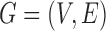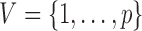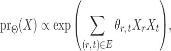The pairwise relationships can be captured by an undirected graph whose vertex set is and whose edge set corresponds to conditional dependencies. The binary Markov random field associated with graph has the joint distribution

(1)

subject to a normalizing constant, where quantifies the conditional dependence between taxa and . With binary , this model has a clear biological interpretation: positive implies co-existence and negative implies co-exclusiveness.

1.2. Differential network analysis

Let and be the matrices that represent the microbial network among discretized taxa abundances for two age groups. In this paper, we are interested in the global test

(2)

If the global null in (2) is rejected, it becomes of interest to test for entrywise changes in the differential network ,

(3)

while controlling the false discovery rate at a prespecified level.

The gut microbial networks of young adults and the elderly often differ only in a small number of links (Goodrich et al., 2016). Our proposed global test uses the maximum of the standardized entrywise differences as the test statistic, and is thus particularly powerful against such sparse alternatives, compared to tests based on the Frobenius norm (Schott, 2007; Li & Chen, 2012). Our multiple testing procedure for differential network analysis accounts for the multiplicity in testing the 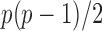hypotheses, with both the false discovery proportion and the false discovery rate controlled asymptotically. The proposed global and multiple testing procedures are implemented in the R package TestBMN (R Development Core Team, 2019), which is available on GitHub. The merits of the proposed tests are further demonstrated through extensive simulations and a gut microbiome study of U.K. twins.

1.3. Our contribution

In an unpublished 2016 technical report from the University of Pittsburgh, Z. Ren developed a method for estimation of individual entries in for a single binary Markov random field model. In contrast, this paper studies global and multiple testing of two Markov random field models with multiple testing error control. Nodewise logistic regressions are used to develop the entrywise test statistics, whose dependence structure is much more complicated than in the Gaussian case (Xia et al., 2015; Cai & Liu, 2016; Xia et al., 2018). The debiased entrywise estimators for testing Gaussian graphical models are based on the residuals from nodewise linear regressions whose correlations are straightforward to characterize. However, the estimators in the current paper depend not only on the residual from each nodewise logistic regression but on carefully defined projection directions needed for bias correction. By overcoming these challenges, we establish theoretical properties of the proposed testing procedures.

2. Global and multiple testing of Markov networks

2.1. Notation and problem set-up

Let be the independent binary observations from the first population and the independent binary observations from the second population, often conveniently written as matrices 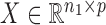and . For a matrix 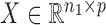, denotes the 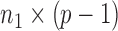submatrix with the th column removed. For a matrix and , let denote the -dimensional subvector of parameters. For a symmetric matrix , and denote the largest and smallest eigenvalues of . For a vector , the usual vector and norms are denoted, respectively, by and . The indicator function is denoted by .

To leverage the sparsity in the differential network , we propose a test based on the maximum of the standardized entrywise differences between the two matrices (Xia et al., 2015). Our motivation is that the global null hypothesis in (2) is equivalent to

Therefore one can construct the test statistic by first obtaining nearly unbiased estimators of 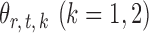and then deriving the standardized entrywise difference , such that

If the global null is rejected, simultaneous testing of entrywise differences is often of interest to identify where the two networks differ. To this end, we also consider multiple testing of all entries in , as formally defined in (3). A natural test statistic for each individual test in (3) is the standardized entrywise difference . For any given threshold level , the null hypothesis is rejected if . Our goal is to choose an optimal threshold such that the proposed multiple testing procedure rejects as many true positives as possible while controlling the false discovery rate at a prespecified level.

2.2. Derivation of the standardized entrywise statistics

To obtain , we first derive nearly unbiased estimators of 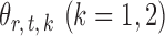and evaluate their variances. Without loss of generality, it suffices to focus on estimation of from .

Given , one can recover the association parameters in a binary Markov random field using -penalized nodewise logistic regression (Ravikumar et al., 2010), because the conditional distribution of given is

(4)

Thus the variable can be viewed as the response in a logistic regression where all remaining variables act as covariates. However, obtained via -penalized estimation (Ravikumar et al., 2010) is biased.

To correct for the bias in , it is instructive to write the th variable as a nonlinear function of all remaining variables, i.e., for every node ,

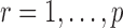(5)

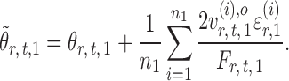
where and are random variables satisfying 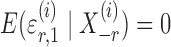. We adopt the projection-based debiasing approach of Zhang & Zhang (2014). Specifically, for a suitably chosen score vector 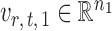and 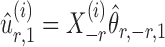, one can show that the estimator

(6)

is nearly unbiased under mild conditions on the initial estimate . The second term on the right-hand side of (6) projects the residual onto the direction of , thereby reducing the bias in to an acceptable level. As shown in the unpublished 2016 technical report by Z. Ren, the desired score vector 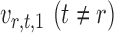can be defined as

(7)

where for ,

Intuitively, the score vector resembles the residual for regressing on . The choice in (7) ensures that is uncorrelated with and that achieves asymptotic efficiency. Given and the initial estimate , the nearly unbiased can be derived similarly.

Remark 1.

Inference for high-dimensional models via the penalty typically requires bias correction, because the regularization achieves variable selection by shrinking every component of the regression coefficients towards zero (Zhang & Zhang, 2014; van de Geer et al., 2014). Existing work on bias correction focuses primarily on linear models, with the exception of van de Geer et al. (2014), which is based on inverting the Karush–Kuhn–Tucker conditions and is applicable to generalized linear models. In contrast, our debiasing approach is based on a local Taylor expansion of about in (5), which yields an approximately linear surrogate to the nonlinear conditional mean and facilitates the construction of entrywise statistics.

The estimators and have unequal variances, so we must adjust for their variances before constructing the test statistic for the global null hypothesis. Denote by the oracle score vector calculated based on ,

and let

By definition, , so . Hence, for a reasonably good initial estimate , one expects to be close to

Indeed, it can be shown that for , under certain conditions. With , one can use as an approximation to .

Finally, let the empirical variance estimates be defined as

The standardized entrywise difference is thus

2.3. Implementation of the testing procedure

Once we have the standardized entrywise statistic , we can construct the test statistic for the global null in (2):

(8)

Section 3.2 shows that under certain mild conditions, converges to a Type I extreme value distribution under the null. Indeed, the are asymptotically standard normal under the null and are only weakly dependent. Hence the maximum of 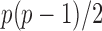such variables squared, that is, , should be close to . Let

(9)

where is the quantile of the Type I extreme value distribution with the cumulative distribution function . We reject the hypothesis whenever .

In the multiple testing problem (3), for any given threshold level and , each individual hypothesis is rejected if . Let denote the set of true nulls. Let be the total number of false positives and the total number of rejections. The false discovery proportion and false discovery rate are defined, respectively, as

For a prespecified level , an ideal choice of that is able to control the false discovery proportion and false discovery rate is

Here the choice of is restricted to because the asymptotic null distribution of is standard normal so that as

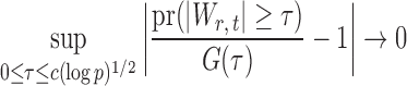
However, the ideal is unavailable because is unknown. To estimate , it is helpful to understand the properties of . Let be the standard normal cumulative distribution function and let . Under the null hypothesis in (3) and some regularity conditions, one can show that as ,

(10)

uniformly for all , where , for any and any . Therefore one can estimate by as in Cai & Liu (2016), where can be estimated by 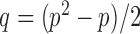due to the sparsity of . In fact, for weakly dependent , it can be shown that

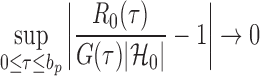(11)

in probability for as . So, we estimate by

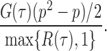This leads to the following estimate of :

(12)

If the solution to (12) does not exist, we set 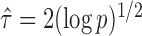. For , the null hypothesis 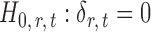is rejected if and only if .

Remark 2.

It is important to restrict in (12) for false discovery proportion control, because the convergence in (11) may not hold for . In such cases, direct thresholding on with is used to control the false discovery rate. Without the constraint , our multiple testing procedure reduces to the Benjamini–Hochberg procedure, which may not control the false discovery proportion with some positive probability if the number of true alternatives is fixed as . An alternative approach to approximating is to bootstrap, as in Cai & Liu (2016).

3. Theoretical properties

3.1. Assumptions

We make assumptions to establish the theoretical properties of the proposed testing procedures. For 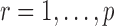, let

denote the Hessians of the likelihood functions associated with the th logistic regression in the first and second populations, respectively. For , the matrix is the Fisher information matrix associated with the local conditional probability distribution, and is analogous to the submatrix of the precision matrix in Gaussian graphical models.

Assumption 1.

Assume that and . For each , there exist constants such that

Further, assume that the initial estimators satisfy

(13)

(14)

The bounded eigenvalue assumption on is standard in inference for high-dimensional Ising models (Ravikumar et al., 2010), and ensures that the variables do not become overly dependent. It is also crucial for establishing the asymptotic normality of . Initial estimators satisfying (13) and (14) can be obtained via -penalized nodewise logistic regression if the maximum node degree is . The conditions in (13) and (14) are slightly stronger than those required for entrywise normality in the unpublished 2016 technical report by Z. Ren, because smaller biases are required for testing procedures in order to provide significance quantification for each pair of edges.

Assumption 2.

For each , there exists a constant such that the maximum neighbourhood weight satisfies

Assumption 2 implies that 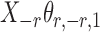and are sub-exponential random variables, and therefore for and some . In view of the conditional distribution (4), violation of Assumption 2 may lead to degenerate marginal distributions. This assumption is crucial for controlling the dependence in Lemma 1, and is also used in Santhanam & Wainwright (2012).

To ensure good performance of the proposed testing procedures, it is important to characterize the dependence between the standardized entrywise statistics and for , and to understand when such dependences are weak. The reason for and being dependent is the correlation among for and . In contrast to the Gaussian case (Xia et al., 2015), it is difficult to evaluate these correlations analytically in the current setting due to the unknown normalizing constant in (1). However, the following lemma says that these correlations are bounded under mild conditions.

Lemma 1.

Under Assumption 2, for and ,

where and are absolute constants that depend only on .

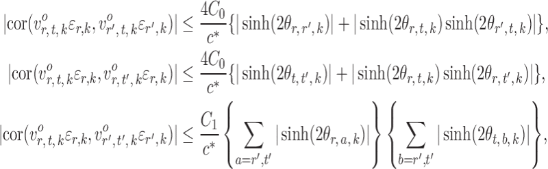
Lemma 1 implies that the correlation among the nearly unbiased estimators , or equivalently the correlation among the , is bounded above by a function of for and . However, establishing such results for high-dimensional binary Markov random fields is challenging. The proof of Lemma 1 requires careful analysis based on the conditional distributions and .

The next assumption requires that the entrywise conditional associations not be too large and ensures that only weakly dependent.

Assumption 3.

For a constant , let

be small enough that for .

Variants of Assumption 3 are commonly used (Cai et al., 2013; Cai & Liu, 2016; Xia et al., 2015, 2018). This assumption is also mild for microbial networks because evolutionary stability and robustness often result in only a small number of strong microbial interactions (Leclerc, 2008).

3.2. Limiting null distribution and optimality of the global test

For , let

denote the set of indices such that either is highly correlated with some or is highly correlated with some , given all remaining variables. Let .

Theorem 1.

Suppose that Assumptions 1–3 hold. If there exist and a sequence of numbers such that , then under the null hypothesis in (2), for any

(15)

as , where is defined in (8). Under the null hypothesis, the convergence in (15) is uniform for all and satisfying Assumptions 1–3.

Remark 3.

The bounded cardinality condition on is similar to that in Cai et al. (2013), and is mild because the magnitude of reflects the conditional association between each pair of microbial taxa. Most of the entries in should be bounded from above, or the rare taxa might go extinct, which is undesirable for maintaining a robust ecological system. This condition together with Assumptions 2 and 3 guarantee weak dependence among the , and allows us to apply strategies for extreme values in the Gaussian case.

In addition to the limiting null distribution, our global testing procedure also maintains rate-optimal power. Consider the matrices

(16)

Let be the set of all -level tests, that is, for any .

Theorem 2.

• (i) Suppose that Assumptions 1–3 hold. The test defined in (2) satisfies

  

  as .
• (ii) Let for and with . Then there exists a constant such that for all sufficiently large and ,

  

Remark 4.

Statement (i) in Theorem 2 says that rejects the null hypothesis in (2) with high probability when , and statement (ii) says that the lower bound of order in (16) cannot be further improved.

3.3. False discovery rate control in multiple testing

Let , let 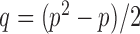, and let

The following theorem shows that our multiple testing procedure ensures asymptotic control of the false discovery proportion and false discovery rate at the prespecified level .

Theorem 3.

Suppose for some and . Assume further that for some and that for some and . Then under the assumptions of Theorem 1,

in probability as .

Remark 5.

The condition on the size of is mild in that it only requires a few standardized entrywise differences to be at least of order , which is necessary to ensure that (11) holds. The proof of Theorem 3 again relies heavily on knowledge of the dependence among the as characterized in Lemma 1.

4. Simulations

4.1. Data and model selection

We consider (a) the Erdős–Rényi random graph (Erdős & Rényi, 1960) with average degree , (b) the Watts–Strogatz model (Watts & Strogatz, 1998), which forms networks with small-world properties, and (c) the Barabasi–Albert scale-free network model (Barabási & Albert, 1999), as illustrated in Fig. 1. In all comparisons, the graph sizes and the sample sizes are taken as and . For a given graph, the nonzero entries were drawn uniformly from . Given the two matrices and , binary data and were generated by Gibbs sampling.

Fig. 1.

Illustrations of different graphs used in our simulations: (a) random graph , (b) small-world network , and (c) scale-free network .

To get an initial estimator of , we run nodewise -regularized logistic regression with penalty parameter , using the R package glmnet (Friedman et al., 2010). Symmetric estimates were obtained by averaging the nodewise estimates. The optimal tuning parameters were chosen to maximize the performance of the global and the multiple testing procedures. For the global test, the tuning parameter in each logistic regression was selected based on the extended Bayesian information criterion (Barber & Drton, 2015). As the multiple testing procedure relies on the approximation of to , the tuning parameters needed in multiple testing were chosen by ensuring was as close to as possible.

4.2. Results

We compare our approach with two-sample testing based on Gaussian graphical models (Xia et al., 2015) and two other permutation-based methods for global testing. The first permutation method uses the same and as in our approach and takes the minimum -value of the entrywise test in (3) as the test statistic. The significance of the global test is then calibrated using a permutation approach. The second permutation method differs from the first only in the way the parameters and are estimated. Specifically, it estimates and its variance using maximum likelihood with specified support of and finite-sample bias correction (Firth, 1993). In our comparisons, the per replication -values for both permutation methods were evaluated over 1000 permutations.

Table 1 presents the empirical Type I errors of the global test, and confirms that our method and the two permutation tests control the Type I errors well in all settings. In comparison, the Type I errors of the method of Xia et al. (2015) are slightly inflated, which is not surprising because the data are not multivariate normal.

Table 1.

Empirical Type I errors and powers of the global test with and . The Type I errors were evaluated over replications, and the powers were calculated over replications

	Method	Type I error			Power
50	Proposed method	3.0	1.6	3.6	94.5	88.0	91.5
	Xia et al. (2015)	8.4	9.4	7.2	69.5	70.0	91.0
	PermBMN	5.8	5.8	5.0	97.0	93.5	96.5
	PermMLE	4.6	5.2	3.8	98.5	97.0	99.5
100	Proposed method	2.0	3.0	2.4	95.5	94.0	97.5
	Xia et al. (2015)	6.2	7.8	7.4	80.0	87.0	94.5
	PermBMN	5.4	5.0	4.2	98.0	97.0	99.0
	PermMLE	4.6	4.8	4.6	97.0	99.0	100.0

PermBMN, permutation-based test using ; PermMLE, permutation-based test using the modified maximum likelihood estimator of assuming that the true graph structures are known.

To evaluate the power of the global test, we constructed the differential network such that five entries in the upper triangular part of were uniformly drawn from . Let be generated from one of the three models or , and let and 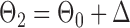. The empirical powers, which are proportions of null hypothesis rejections, are shown in Table 1. Our method yields very high powers for all settings and uniformly outperforms the method of Xia et al. (2015). The two permutation-based methods, especially the second one based on the modified maximum likelihood estimator of , demonstrate superior performance in terms of power. The downside is that both permutation methods require heavy computation.

Finally, using the same design and 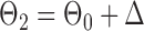, we examined multiple testing of individual entries in the differential network while controlling the false discovery rate at . The true differential network was constructed to be sparse such that the number of edges is approximately , with nonzero entries drawn uniformly from . The empirical false discovery and true positive rates of our method and that of Xia et al. (2015) were estimated by

where denotes the set of nonzero locations. Permutation-based methods are inapplicable to multiple testing. Table 2 shows that our multiple testing procedure controls the false discovery rate well in all scenarios, and returns reasonably high true positive rates. In contrast, the multiple testing method of Xia et al. (2015) yields slightly higher false positive and lower true positive rates. The difference in true positive rates between the methods increases with .

Table 2.

Empirical false discovery rates and true positive rates for multiple testing with false discovery rate and over replications

	Method	False discovery rate			True positive rate
50	Proposed method	10.0	9.1	10.6	52.9	59.9	61.0
	Xia et al. (2015)	13.8	13.7	13.5	51.7	54.9	59.9
100	Proposed method	8.3	9.4	9.2	56.1	57.7	62.9
	Xia et al. (2015)	12.2	12.3	11.7	50.5	49.6	57.2

5. Application to gut microbiome data in U.K. twins

We applied the proposed testing procedures to data from a gut microbiome study of U.K. twins. The original study (Goodrich et al., 2016) investigated whether host genotype shapes the gut microbiome composition, using 16S rRNA sequencing data collected from faecal samples of 2731 individuals. The data are available at http://www.ebi.ac.uk/ena/data/view/PRJEB13747. We are interested in whether the microbial community structures summarized as conditional dependence relationships among the microbial taxa are associated with the age of the host.

To ensure robust detection of microbial interactions, samples with total read counts less than 20 were first removed. For each of the remaining samples, the relative abundance of each genus was calculated by dividing the read count for each genus by the total number of reads in the sample. Of the 294 genera, only those with at least 0.001% of relative abundance in at least 75% of the 2714 samples were used, which reduces the total number of genera to . To examine the association of microbial interactions with host age, we selected 286 young adults who were at most 43 years and 284 elderly subjects aged at least 74 years. Since these samples included twins, we randomly chose one individual from each pair of twins, which gave independent young adults and elderly subjects in our analysis.

Because of possible errors in sequencing reads, genera with relative abundance lower than are expected to be due to noise or sequencing errors. We therefore first discretized the relative abundances using a cut-off of 0.001%, where for a given genus, represents absence or extremely low abundance of the genus and represents presence. However, some more abundant genera are present in over 75% of the samples. For these genera, we used the 25th percentile as the cut-off to discretize the data, so represents low abundance of the genus and represents high abundance. One should keep the definitions in mind when interpreting the parameters.

We applied the global testing procedure to the two groups of subjects and obtained a -value of 0.009, indicating that the microbial networks for the two age groups are significantly different. To assess the stability of our method and perform power comparisons, we generated 1000 subsamples within each age group, with sampling proportions ranging from to . The empirical powers of our method and the permutation method using are presented in Fig. 2(a). Our method performs slightly worse than the permutation method, but we believe that the gap reduces with larger samples. Another advantage of our method is that it runs much faster than the permutation method. We also performed back-testing for the global null hypothesis by randomly splitting the pooled data into two groups with and subjects over 1000 replications. Figure 2(b) shows the resulting -values, which are slightly skewed towards the right, indicating that the proposed test is conservative.

Fig. 2.

(a) Empirical power curves of the proposed method (circles) and the permutation method using (triangles) by subsampling the two datasets at different proportions. (b) A histogram of the -values from our method in back-testing by randomly generating two datasets 1000 times.

To recover the differential microbial network, we applied the proposed multiple testing procedure with and show the results in Fig. 3. The same differential links were selected by fdr between 14% to 16%. For fdr between 12% to 14%, all edges in Fig. 3 except that between Bacteroides and Blautia were selected. Here the two values associated with each differential edge represent the estimated odds ratios between the two genera for the two age groups. For example, the odds ratio between Faecalibacterium and Campylobacter among young adults is , indicating that high abundance in Faecalibacterium is associated with lower odds of high abundance in Campylobacter. In other words, Faecalibacterium and Campylobacter have a competitive relationship within the microbial community, which could be due to their competition for space, nutrients, and so on. In contrast, the relationship between Faecalibacterium and Campylobacter is collaborative for the elderly group, since the odds ratio is . A collaborative relationship between two microbes can be due to cross-feeding, co-colonization or other reasons (Faust & Raes, 2012). Each pair of values associated with each edge shows a significant difference, suggesting changes in the microbial community structure as people age. Indeed, the abundance of Faecalibacterium has been found to be negatively associated with age (Franceschi et al., 2017). Further, Ruminococcus was significantly enriched in immune-mediated inflammatory diseases (Forbes et al., 2016), and Oscillospira was enriched in inflammatory diseases (Konikoff & Gophna, 2016). Thus Ruminococcus and Oscillospira may also play an important role in the ageing process, because age is characterized by chronic low-grade inflammation. Figure 3 provides additional evidence on how these genera are implicated in the ageing process. More importantly, genera involved in the differential network may be potential microbial targets that can be manipulated through dietary or medical interventions for healthy ageing. As the true differential network is unknown, further experimental validation is needed to confirm these results.

Fig. 3.

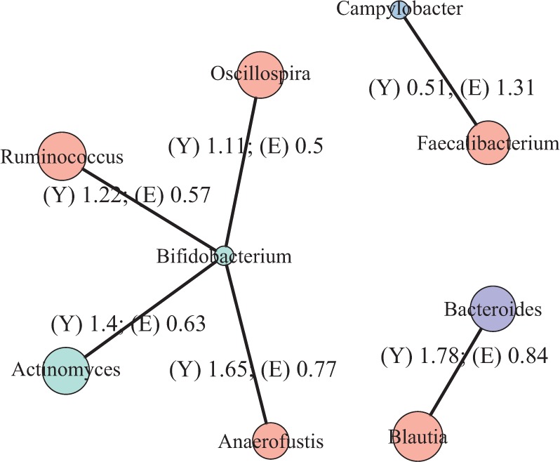
Estimated differential microbial network between young and elderly individuals using our multiple testing procedure with fdr = 15%, where isolated genera are not shown. Each node represents a genus coloured by phylum, and node size is proportional to the prevalence of 1s among all samples for the corresponding genus. Edge width is proportional to the magnitude of the entrywise test statistic. Turquoise circles, Actinobacteria; purple circles, Bacteroidetes; red circles, Firmicutes; blue circles, Proteobacteria.

Since the method of Xia et al. (2015) does not perform well for discrete data, we applied their method to the centred log-ratio transformed relative abundance data and obtained a -value of 0.007 for the global test, which is consistent with the conclusion from the proposed global test. At 15% false discovery rate, application of the multiple testing procedure of Xia et al. (2015) only gave one differential edge between Holdemania from the phylum Firmicutes and Butyricimonas from Bacteroidetes. The difference is largely due to the fact that the centred log-ratio transformed data are far from being normally distributed.

6. Discussion

To deal with excessive zeros and the unit sum constraint, in this paper we proposed using a binary Markov random field to study microbial interactions characterized by their conditional dependence relationships. Such models are robust and largely free of distributional assumptions on the data and have a natural interpretation in terms of co-existence or co-exclusiveness of the microbial communities. For very rare taxa, we suggest using a very small cut-off to discretize the data. For more common taxa, sample median or quartiles can be used. Using different cut-offs may lead to different results and thus to models with different interpretations. One may explore different ways of dichotomizing the data to see whether consistent results can be obtained.

The proposed method for testing binary Markov random fields can be applied to other data with binary observations, such as cancer somatic mutation data in cancer genomics or characterization of neural firing patterns and the reconstruction of neural connections in neuroscience. Our methods can be extended to study more general Markov random fields with each node taking more than two discrete values.

Supplementary material

Supplementary material available at Biometrika online includes technical lemmas and proofs.

References

- Aitchison, J. (1982). The statistical analysis of compositional data (with discussion). J. R. Statist. Soc. B 44, 139–77. [Google Scholar]
- Barabási, A.-L. & Albert, R. (1999). Emergence of scaling in random networks. Science 286, 509–12. [DOI] [PubMed] [Google Scholar]
- Barber, R. F. & Drton, M. (2015). High-dimensional Ising model selection with Bayesian information criteria. Electron. J. Statist. 9, 567–607. [Google Scholar]
- Biagi, E., Nylund, L., Candela, M., Ostan, R., Bucci, L., Pini, E., Nikkïla, J., Monti, D., Satokari, R., Franceschi, C.. et al. (2010). Through ageing, and beyond: Gut microbiota and inflammatory status in seniors and centenarians. PLoS One 5, 1–14. [DOI] [PMC free article] [PubMed] [Google Scholar]
- Biswas, S., McDonald, M., Lundberg, D. S., Dangl, J. L. & Jojic, V. (2016). Learning microbial interaction networks from metagenomic count data. J. Comp. Biol. 23, 526–35. [DOI] [PubMed] [Google Scholar]
- Cai, T. T. & Liu, W. (2016). Large-scale multiple testing of correlations. J. Am. Statist. Assoc. 111, 229–40. [DOI] [PMC free article] [PubMed] [Google Scholar]
- Cai, T. T., Liu, W. & Xia, Y. (2013). Two-sample covariance matrix testing and support recovery in high-dimensional and sparse settings. J. Am. Statist. Assoc. 108, 265–77. [Google Scholar]
- Claesson, M. J., Cusack, S., O’Sullivan, O., Greene-Diniz, R., de Weerd, H., Flannery, E., Marchesi, J. R., Falush, D., Dinan, T., Fitzgerald, G.. et al. (2011). Composition, variability, and temporal stability of the intestinal microbiota of the elderly. Proc. Nat. Acad. Sci. 108, 4586–91. [DOI] [PMC free article] [PubMed] [Google Scholar]
- Erdős, P. & Rényi, A. (1960). On the evolution of random graphs. Pub. Math. Inst. Hungar. Acad. Sci. 5, 17–61. [Google Scholar]
- Fang, H., Huang, C., Zhao, H. & Deng, M. (2017). gCoda: Conditional dependence network inference for compositional data. J. Comp. Biol. 24, 699–708. [DOI] [PMC free article] [PubMed] [Google Scholar]
- Faust, K. & Raes, J. (2012). Microbial interactions: From networks to models. Nat. Rev. Microbiol. 10, 538–50. [DOI] [PubMed] [Google Scholar]
- Firth, D. (1993). Bias reduction of maximum likelihood estimates. Biometrika 80, 27–38. [Google Scholar]
- Forbes, J. D., Van Domselaar, G. & Bernstein, C. N. (2016). The gut microbiota in immune-mediated inflammatory diseases. Front. Microbiol. 7, 1081. [DOI] [PMC free article] [PubMed] [Google Scholar]
- Franceschi, C., Garagnani, P., Vitale, G., Capri, M. & Salvioli, S. (2017). Inflammaging and ‘garb-aging’. Trends Endocrinol. Metab. 28, 199–212. [DOI] [PubMed] [Google Scholar]
- Friedman, J. H., Hastie, T. J. & Tibshirani, R. J. (2010). Regularization paths for generalized linear models via coordinate descent. J. Statist. Software 33, 1–22. [PMC free article] [PubMed] [Google Scholar]
- Goodrich, J. K., Davenport, E. R., Beaumont, M., Jackson, M. A., Knight, R., Ober, C., Spector, T. D., Bell, J. T., Clark, A. G. & Ley, R. E. (2016). Genetic determinants of the gut microbiome in UK twins. Cell Host & Microbe 19, 731–43. [DOI] [PMC free article] [PubMed] [Google Scholar]
- Konikoff, T. & Gophna, U. (2016). Oscillospira: A central, enigmatic component of the human gut microbiota. Trends Microbiol. 24, 523–4. [DOI] [PubMed] [Google Scholar]
- Kuczynski, J., Lauber, C. L., Walters, W. A., Parfrey, L. W., Clemente, J. C., Gevers, D. & Knight, R. (2012). Experimental and analytical tools for studying the human microbiome. Nat. Rev. Genet. 13, 47–58. [DOI] [PMC free article] [PubMed] [Google Scholar]
- Kurtz, Z. D., Müller, C. L., Miraldi, E. R., Littman, D. R., Blaser, M. J. & Bonneau, R. A. (2015). Sparse and compositionally robust inference of microbial ecological networks. PLoS Comp. Biol. 11, 1–25. [DOI] [PMC free article] [PubMed] [Google Scholar]
- Leclerc, R. D. (2008). Survival of the sparsest: Robust gene networks are parsimonious. Molec. Syst. Biol. 4, 213. [DOI] [PMC free article] [PubMed] [Google Scholar]
- Li, J. & Chen, S. X. (2012). Two sample tests for high-dimensional covariance matrices. Ann. Statist. 40, 908–40. [Google Scholar]
- R Development Core Team (2019). R: A Language and Environment for Statistical Computing. Vienna, Austria: R Foundation for Statistical Computing; ISBN 3-900051-07-0, http://www.R-project.org. [Google Scholar]
-
Ravikumar, P., Wainwright, M. J. & Lafferty, J. D. (2010). High-dimensional Ising model selection using
-regularized logistic regression. Ann. Statist. 38, 1287–319. [Google Scholar]
- Santhanam, N. P. & Wainwright, M. J. (2012). Information-theoretic limits of selecting binary graphical models in high dimensions. IEEE Trans. Info. Theory 58, 4117–34. [Google Scholar]
- Schott, J. R. (2007). A test for the equality of covariance matrices when the dimension is large relative to the sample sizes. Comp. Statist. Data Anal. 51, 6535–42. [Google Scholar]
- van de Geer, S., Bühlmann, P., Ritov, Y. & Dezeure, R. (2014). On asymptotically optimal confidence regions and tests for high-dimensional models. Ann. Statist. 42, 1166–202. [Google Scholar]
- Watts, D. J. & Strogatz, S. H. (1998). Collective dynamics of small-world networks. Nature 393, 440–2. [DOI] [PubMed] [Google Scholar]
- Xia, Y., Cai, T. & Cai, T. T. (2015). Testing differential networks with applications to the detection of gene-gene interactions. Biometrika 102, 247–66. [DOI] [PMC free article] [PubMed] [Google Scholar]
- Xia, Y., Cai, T. & Cai, T. T. (2018). Multiple testing of submatrices of a precision matrix with applications to identification of between pathway interactions. J. Am. Statist. Assoc. 113, 328–39. [DOI] [PMC free article] [PubMed] [Google Scholar]
- Zhang, C.-H. & Zhang, S. S. (2014). Confidence intervals for low dimensional parameters in high dimensional linear models. J. R. Statist. Soc. B 76, 217–42. [Google Scholar]
Associated Data
This section collects any data citations, data availability statements, or supplementary materials included in this article.